Parallel computing principles and practice pdf

This book sets out the principles of parallel computing in a way
which will be useful to student and potential user alike. It includes
coverage of both conventional and neural computers. The content
of the book is arranged hierarchically. It explains why, where and
how parallel computing is used; the fundamental paradigms
employed in the field; how systems are programmed or trained;
technical aspects including connectivity and processing element
complexity; and how system performance is estimated (and why
doing so is difficult).
The penultimate chapter of the book comprises a set of
case
studies
of archetypal parallel computers, each study written by an individ-
ual closely connected with the system in question. The final chap-
ter correlates the various aspects of parallel computing into a tax-
onomy of systems.
Parallel computing
principles and practice
Parallel computing
principles
and
practice
T.
J.
FOUNTAIN
Department
of
Physics
and Astronomy, University College London

CAMBRIDGE
UNIVERSITY PRESS
CAMBRIDGE UNIVERSITY PRESS
Cambridge, New York, Melbourne, Madrid, Cape Town, Singapore, Sao Paulo
Cambridge University Press
The Edinburgh Building, Cambridge CB2 2RU, UK
Published in the United States of America by Cambridge University Press, New York
www. c ambridge. org
Information on this title: www.cambridge.org/9780521451314
© Cambridge University Press 1994
This publication is in copyright. Subject to statutory exception
and to the provisions of relevant collective licensing agreements,
no reproduction of
any
part may take place without
the written permission of Cambridge University Press.
First published 1994
This digitally printed first paperback version 2006
A
catalogue
record for
this publication
is available from
the British
Library
Library of
Congress Cataloguing
in
Publication
data

Fountain, T. J. (Terry J.)
Parallel computing
:
principles and practice /
T.
J. Fountain.
p.
cm.
Includes bibliographical references and index.
ISBN
0-521-45131-0
1.
Parallel processing (Electronic computers) I. Title.
QA76.58.F67 1994
004
f
.35-dc20 93-36763 CIP
ISBN-13 978-0-521-45131-4 hardback
ISBN-10
0-521-45131-0
hardback
ISBN-13 978-0-521-03189-9 paperback
ISBN-10
0-521-03189-3
paperback
Contents
Preface
xi
1 Introduction
1

1.1
Basic approaches
4
1.1.1
Programmed systems
4
1.1.2
Trainable systems
14
1.2
Fundamental system aspects
17
1.3
Application areas
18
1.3.1
Image processing
19
1.3.2
Mathematical modelling
21
1.3.3
Artificial intelligence
25
1.3.4
General database manipulation
27
1.4
Summary
28

2 The Paradigms
of
Parallel Computing
30
31
32
37
41
47
52
59
64
70
71
72
74
75
77
78
Programming Parallel Computers
80
3.1 Parallel programming
80
3.1.1 The embodiment of parallelism
80
3.1.2 The programming paradigm
84
3.1.3 The level
of
abstraction

94
2.1
2.2
2.3
2.4
2.5
2.6
2.7
2.8
2.9
2.10
2.11
2.12
Flynn's taxonomy
Pipelining
MIMD
Graph reduction
SIMD
Systolic
Association
Classification
Transformation
Minimisation
2.10.1
Local minimisation
2.10.2
Global minimisation
Confusion compounded
2.11.1
The vector supercomputer

Exercises
Vll
viii Contents
3.2 Parallel languages
3.2.1 Fortran
3.2.2 Occam
3.2.3 Parlog
3.2.4 Dactl
3.3 Cognitive training
3.3.1 Hebb'srule
3.3.2 Simulated annealing
3.3.3 Back propagation
3.4 Conclusions
3.5 Exercises
Connectivity
4.1 Synchronising communications
4.2 The role of memory
4.3 Network designs
4.3.1 The bus
4.3.2 The crossbar switch
4.3.3 Near neighbours
4.3.4 Trees and graphs
4.3.5 The pyramid
4.3.6 The hypercube
4.3.7 Multistage networks
4.3.8 Neural networks
4.4 Reconfigurable networks
4.5 System interconnections
4.6 Conclusions
4.7 Exercises

Processor Design
5.1 Analogue or digital?
5.2 Precision
5.3 Autonomy
5.3.1 Variously-autonomous processors
5.4 Instruction set complexity
5.5 Technology
5.5.1 Basic materials
5.5.2 Device types
5.5.3 Scale of fabrication
5.6 Three design studies
5.6.1 An MIMD computer for general scientific computing
5.6.2 An SIMD array for image processing
5.6.3 A cognitive network for parts sorting
103
104
106
108
109
111
113
115
118
120
121
123
124
126
130
134

138
139
143
147
150
153
155
159
161
162
164
166
166
168
170
171
174
174
175
176
176
177
178
182
188
Contents ix
190
191
193
194

194
195
195
195
195
196
196
197
199
202
203
205
206
207
208
210
220
220
220
221
221
222
Some Case Studies 224
7A Datacube contributed by D. Simmons 226
7B Cray contributed by J. G. Fleming 236
7C nCUBE contributed by R. S. Wilson 246
7D Parsys contributed by D. M. Watson 256
7E GRIP contributed by C. Clack 266
7F AMT DAP contributed by D. J. Hunt 276
7G MasPar MP-1 contributed by J. R. Nickolls 287

7H WASP contributed by I. Jaloweicki 296
71 WISARD contributed by C. Myers 309
Conclusions 320
8.1 A taxonomy of systems 320
8.2 An analysis of alternatives 326
5.7
5.8
Conclusions
Exercises
System Performance
6.1
6.2
6.3
6.4
6.5
6.6
6.7
6.8
6.9
Basic performance measures
6.1.1 Clock rate
6.1.2 Instruction rate
6.1.3 Computation rate
6.1.4 Data precision
6.1.5 Memory size
6.1.6 Addressing capability
Measures of data communication
6.2.1 Transfer rate
6.2.2 Transfer distance
6.2.3 Bottlenecks

Multiplication factors
The effects of software
Cognitive systems
Benchmarking
6.6.1 A brief survey of benchmarks
6.6.2 Case studies
Defining and measuring costs
6.7.1 Hardware
6.7.2 Software
6.7.3 Prototyping and development
Summary and conclusions
Exercises
Contents
8.2.1
8.2.2
8.2.3
8.2.4
8.2.5
The user interface
Generality of application
Technical issues
Efficiency
Summary
8.3 The future
8.3.1
8.3.2
8.3.3
8.3.4
Commercial
Architectures

Technology
User interfaces
8.4 Concluding remarks
Bibliography
References
Index
326
328
330
331
332
332
333
334
334
336
336
337
338
343
Preface
The study of parallel computing is just about as old as that of computing
itself.
Indeed, the early machine architects and programmers (neither cate-
gory would have described themselves in these terms) recognised no such
delineations in their work, although the natural human predilection for
describing any process as a sequence of operations on a series of variables
soon entrenched this philosophy as the basis of
all
normal systems.

Once this basis had become firmly established, it required a definite effort
of will to perceive that alternative approaches might be worthwhile, espe-
cially as the proliferation of potential techniques made understanding more
difficult. Thus, today, newcomers to the field might be told, according to
their informer's inclination, that parallel computing means the use of trans-
puters, or neural networks, or systolic arrays, or any one of a seemingly
endless number of possibilities. At this point, students have the alternatives
of accepting that a single facet comprises the whole, or attempting their
own processes of analysis and evaluation. The potential users of a system
are as likely to be set on the wrong path as the right one toward fulfilling
their own set of practical aims.
This book is an attempt to set out the general principles of parallel com-
puting in a way which will be useful to student and user alike. The approach
I adopt to the subject is top-down - the simplest and most fundamental
principles are enunciated first, with each important area being subsequently
treated in greater depth. I would also characterise the approach as an
engineering one, which flavours even the sections on programming parallel
systems. This is a natural consequence of
my
own background and training.
The content of the book is arranged hierarchically. The first chapter
explains why parallel computing is necessary, where it is commonly used,
why the reader needs to know about it, the two or three underlying
approaches to the subject and those factors which distinguish one system
from another. The fundamental paradigms of parallel computing are set out
in the following chapter. These are the key methods by which the various
approaches are implemented - the basic intellectual ideas behind particular
implementations. The third chapter considers a matter of vital importance,
namely how these ideas are incorporated in programming languages.
The next two chapters cover fundamental technical aspects of parallel

xi
xii Preface
computers - the ways in which elements of parallel computers are connect-
ed together, and the types of processing element which are appropriate for
different categories of system.
The following chapter is of particular significance. One (perhaps the only)
main reason for using parallel computers is to obtain cost-effectiveness or
performance which is not otherwise available. To measure either parameter
has proved even more difficult for parallel computers than for simpler
systems. This chapter seeks to explain and mitigate this difficulty.
The penultimate chapter of the book comprises a set of case studies of
archetypal parallel computers. It demonstrates how the various factors
which have been considered previously are drawn together to form coherent
systems, and the compromises and complexities which are thereby engen-
dered. Each study has been written by an individual closely connected with
the system in question, so that a variety of different factors are given promi-
nence according to the views of each author.
The final chapter correlates the various aspects of parallel computing into
a taxonomy of systems and attempts to develop some conclusions for the
future.
Appropriate chapters are followed by exercises which are designed to
direct students' attention towards the most important aspects of each area,
and to explore their understanding of each facet. At each stage of the book,
suggestions are made for further reading, by means of which interested
readers may extend the depth of their knowledge. It is the author's hope
that this book will be of use both to students of the subject of parallel com-
puting and to potential users who want to avoid the many possible pitfalls
in understanding this new and complex field.
1 Introduction
Before attempting to understand the complexities of the subject of parallel

computing, the intending user or student ought, perhaps, to ask why such
an exotic approach is necessary. After all, ordinary, serial, computers are in
successful and widespread use in every area of society in industrially devel-
oped nations, and obtaining a sufficient understanding of their use and
operation is no simple task. It might even be argued that, since the only rea-
son for using two computers in place of one is because the single device is
insufficiently powerful, a better approach is to increase the power (presum-
ably by technological improvements) of
the
single machine.
As is usually the case, such a simplistic approach to the problem conceals
a number of significant points. There are many application areas where the
available power of 'ordinary' computers is insufficient to obtain the desired
results. In the area of computer vision, for example, this insufficiency is
related to the amount of time available for computation, results being
required at a rate suitable for, perhaps, autonomous vehicle guidance. In
the case of weather forecasting, existing models, running on single comput-
ers,
are certainly able to produce results. Unfortunately, these are somewhat
lacking in accuracy, and improvements here depend on significant exten-
sions to the scope of the computer modelling involved. In some areas of
sci-
entific computation, including those concerned with the analysis of funda-
mental particle interactions, the time scale of the computation on current
single computers would be such as to exceed the expected time to failure of
the system.
In all these cases, the shortfall in performance is much greater than might
at first be supposed - it can easily be several orders of
magnitude.
To take a

single example from the field of image processing, it was recently suggested
to me that operatives of a major oil company, when dealing with seismic
data, would wish to have real-time processing of
10
9
voxels of
data.
(A voxel
is an elemental data volume taken from a three-dimensional image.) This
implies a processing rate of the order of 10
12
operations per second.
Compare this with the best current supercomputers, offering about 10
10
operations per second (which themselves utilise a variety of parallel tech-
niques as we shall see later) and the scale of the problem becomes apparent.
Although technological advance is impressively rapid, it tends to be only
1
2 Introduction
about one order of magnitude every decade for general-purpose computers
(but see Chapter 6 concerning the difficulties of measuring and comparing
performance). Furthermore, the rate of technological improvement is show-
ing signs of falling off as fundamental physical limits are approached and
the problems of system engineering become harder, while the magnitude of
some of the problems is becoming greater as their true requirements are bet-
ter understood.
Another point concerns efficiency (and cost-effectiveness). Serial comput-
ers have a number of conceptual drawbacks in some of the application
areas we are considering. These are mainly concerned with the fact that the
data (or the problem) often has a built-in structure which is not reflected in

the serial computer. Any advantage which might accrue by taking this
structure into account is first discarded (by storing three-dimensional data
as a list, for example) and then has to be regained in some way by the pro-
grammer. The inefficiency is therefore twofold - first the computer manipu-
lates the data clumsily and then the user has to work harder to recover the
structure to understand and solve the problem.
Next, there is the question of storage and access of
data.
A serial comput-
er has, by definition, one (for the von Neumann architecture) or two (in the
case of the Harvard system) channels to its memory. The problem outlined
above in the field of image processing would best be solved by allowing
simultaneous access to more than one million data items, perhaps in the
manner illustrated in Figure 1.1. It is at least arguable that taking advan-
tage of this possibility in some parallel way would avoid the serious prob-
lem of the processor-memory bottleneck which plagues many serial systems.
Finally, there is the undeniable existence of parallelism, on a massive
scale, in the human brain. Although it apparently works in a very different
way from ordinary computers, the brain is a problem-solver of unsurpassed
excellence.
There is, then, at least aprima facie case for the utility of parallel comput-
ing. In some application areas, parallel computers may be easier to pro-
gram, give performance unobtainable in any other way, and might be more
cost-effective than serial alternatives. If this case is accepted, it is quite rea-
sonable that an intending practitioner in the field should need to study and
understand its complexities. Can the same be said of an intending user?
Perhaps the major problem which faces someone confronting the idea of
parallel computing for the first time is that it is not a single idea. There are
at least half a dozen significantly different approaches to the application of
parallelism, each with very different implications for the user. The worst

aspect of this is that, for a particular problem, some approaches can be seri-
ously counter-productive. By this I mean that not only will some techniques
be less effective than others, but some will be worse than staying with con-
ventional computing in the first place. The reason is one which has been
(a)
Program
Data
CPU
Program
Data
CPU
Introduction
(b)
Array of
Memory Elements
Figure 1.1 Overcoming the serial computer data bottleneck (a) von Neumann
(b) Harvard (c) Parallel
mentioned already, namely that the use of parallelism almost always
involves an attempt to improve the mapping between a computer and a par-
ticular class of problem. The kernel of
the
matter, then, is this:
In order to understand parallel computing, it is necessary to understand
the relationships between problems and systems.
One starting point might be to consider what application areas could
benefit from the use of parallelism. However, in order to understand why
these are suggested as being appropriate, it is first necessary to know some-
thing about the different ways in which parallelism can be applied.
4 Introduction
1.1 Basic approaches

Fortunately, at this stage, there are only three basic approaches which we
need to consider. As a first step, we need to differentiate between pro-
grammed and trained systems. In a programmed system, the hardware and
software are conceptually well separated, i.e. the structure of the machine
and the means by which a user instructs it are considered to be quite inde-
pendent. The hardware structure exists, the user writes a program which
tells the hardware what to do, data is presented and a result is produced. In
the remainder of this book, I will often refer to this idea as
calculation.
In a
trainable system, on the other hand, the method by which the system
achieves a given result is built into the machine, and it is trained by being
shown input data and told what result it should produce. After the training
phase, the structure of the machine has been self-modified so that, on being
shown further data, correct results are produced. This basic idea will often
be referred to as
cognition
in what follows.
The latter approach achieves parallel embodiment in structures which are
similar to those found in the brain, in which parallelism of data and func-
tion exist side by side. In programmed systems, however, the two types of
parallelism tend to be separated, with consequent impact on the functioning
of the system. There are therefore three basic approaches to parallel com-
puting which we will now examine - parallel cognition (PC), data parallel
calculation (DPC) and function parallel calculation (FPC). In order to clar-
ify the differences between them, I will explain how each technique could be
applied to the same problem in the field of computer vision and, as a start-
ing point, how a serial solution might proceed.
The general problem I consider is how to provide a computer system
which will differentiate between persons 'known' to it, whom it will permit

to enter a secure area, and persons that it does not recognise, to whom it
will forbid entry. We will assume that a data input system, comprising a
CCTV and digitiser, is common to all solutions, as is a door opening device
activated by a single signal. To begin, let us consider those aspects which
are shared by all the programmed approaches.
7.7.7 Programmed
systems
The common components of a programmable computer system, whatever
its degree of parallelism, are illustrated in Figure 1.2. They comprise one or
more data stores; one or more computational engines; at least one program
store, which may or may not be contiguous with the data store(s); and one
or more program sequencers. In addition to these items of hardware, there
will be a software structure of variable complexity ranging from a single,
executable program to a suite including operating system, compilers and
1.1 Basic approaches 5
Program
Store
Data
Store
Program
Sequencer
Computing
Engine
Executable Programs
Compiler
User Programs
Editor
Operating System
Figure 1.2 The common components of programmable systems
executable programs. Leaving aside the variability, the structure is simply

program, store, sequencer and computer. How are these components
employed to solve the problem in hand?
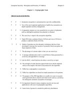
LI.
1.1
Serial
The data which is received from the combination of camera and digitiser
will be in the form of a continuous stream of (usually) eight-bit numbers,
changing at a rate determined by the clock rate of the digitiser. This should,
ideally, be very high (of the order of 50 MHz) in order to reproduce faith-
fully the high-frequency components of the information in the image. The
first requirement is to store this data in a form which will both represent the
image properly and be comprehensible to the computer. This is done by
considering the image as a set of pixels - sub-areas of the image sufficiently
small that the information they contain can be represented by a single num-
ber, called the grey-level of the pixel. The data stream coming from the digi-
tiser is sampled at a series of points such that the stored data represents a
square array of pixels similar to those shown in Figure 1.3. The pixel values
may be stored in either a special section of
memory,
or in part of
the
general
computer memory. In either case they effectively form a list of data items.
The computer will contain and, when appropriate, sequence a program of
instructions to manipulate this list of data to obtain the required result. A
general flow chart of the process might be that shown in Figure 1.4 - each
block of the chart represents an operation (or group of operations) on
Introduction
• ••'
4PPP

MM:
0
0
3
0
1
L
0
6
3
1
•
0
7
3
0
8
1
1
0 0
9
1
1
9
1
=
0
9
1
0

9
1
7
0_
0
0
2
0
0
0
0
9
1
7
0_
0
0
2
0
0
0
0
8
7
1
5
5_
0
2
0

0
0
0
0
6
7
1
1
0_
5
0
0
0
0
0
0
0
0
0
0
0_
0
0
0
0
0
0
o o o o o o o
1
I 1 1 1 1 1

0
0
0
0
0
Figure 1.3 An image represented as an array of square pixels
either the original image data or on some intermediate result. At each stage,
each instruction must be executed on a series of items, or sets of items, of
data until the function has been applied to the whole image. Consider the
first operation shown, that of filtering the original data. There are many
ways of doing this, but one method is to replace the value of each pixel with
the average value of the pixels in the local spatial neighbourhood. In order
to do this, the computer must calculate the set of addresses corresponding
to the neighbourhood for the first pixel, add the data from these addresses,
divide by the number of
pixels
in the neighbourhood, and store the result as
the first item of a new list. The fact that the set of source addresses will not
be contiguous in the address space is an added complication. The computer
must then repeat these operations until the averaging process has been
applied to every part of the original data. In a typical application, such as
we envisage here, there are likely to be more than 64 000 original pixels, and
therefore almost that number of averaging operations. Note that all this
effort merely executes the
first
filtering
operation in the
flow
chart!
However, things are not always so bad. Let us suppose that the program

has been able to segment the image - that is, the interesting part (a human
face) has been separated from the rest of the picture. Already at this stage
1.1 Basic approaches 7
Input data
Output data
Filter
Segment
Measure
Mat
Data
tch
base
Figure 1.4 A serial program flow chart
the amount of data to be processed, although still formidable, has been
reduced, perhaps by a factor of 10. Now the program needs to find the
edges of
the
areas of interest in the face. Suitable subsets (again, local neigh-
bourhoods) of the reduced data list must be selected and the gradients of
the data must be computed. Only those gradients above some threshold
value are stored as results but, along with the gradient value and direction,
information on the position of the data in the original image must be
stored. Nevertheless, the amount of data stored as a result of this process is
very significantly reduced, perhaps by a factor of 100.
Now the next stages of the flow chart can be executed. Certain key dis-
tances between points of the edge map data are computed as parameters of
the original input - these might be length and width of the head, distance
between the eyes, position of the mouth, etc. At this stage the original input
picture has been reduced to a few (perhaps 10) key parameters, and the final
stage can take place - matching this set of parameters against those stored

in a database of known, and therefore admissible, persons. If no match is
found, admittance is not granted.
A number of points are apparent from a consideration of the process
described above. First, a very large number of computations are required to
process the data from one image. Although it is unlikely that a series of
would-be intruders would present themselves at intervals of less than a few
seconds, it must be borne in mind that not all images obtained from the
camera during this period will be suitable for analysis, so the required repe-
tition rate for processing may be much faster than once every second. This
is going to make severe demands on the computational speed of a serial
8 Introduction
computer, especially if the program is sufficiently complex to avoid unac-
ceptable rates of error.
Second, the amount of data which needs to be stored and accessed is also
very large - a further point which suggests that some form of parallel pro-
cessing might be suitable.
Third, at least two possible ways can be discerned in which parallelism
might be applied - at almost every stage of the process data parallelism
could be exploited, and at several places
functional
parallelism could be of
benefit. In the following sections we shall see how each of these approaches
might be used, but it is necessary to continually bear in mind that a pro-
grammed parallel computing system comprises three facets - hardware
(self-evidently), software (which enables the user to take advantage of the
parallelism) and algorithms (those combinations of machine operations
which efficiently execute what the user wants to do). Disregarding any one
of the three is likely to be counter-productive in terms of achieving results.
1.1.1.2
Parallel data

In this and the next two sections I shall assume that cost is no object in the
pursuit of performance and understanding. Of course, this is almost never
the case in real life, but the assumption will enable us to concentrate on
developing some general principles. We might note, in passing, that the first
of these could be:
Building a parallel computer nearly always costs more than building
a
serial one
- but it may
still be more cost-effective
!
I have already stated that all our systems share a common input compris-
ing CCTV and digitiser, so our initial data format is that of a string of
(effectively) pixel values. Before going any further with our design, we must
consider what we are attempting to achieve. In this case, we are seeking out
those areas of our system design where data parallelism may be effectively
applied, and this gives us a clue as to the first move. This should be to carry
out an analysis of the parallel data types in our process, and the relation-
ships between them. Our tool for doing this is the data format flow chart,
shown in Figure 1.5.
The chart is built up as follows. Each node of the chart (a square box)
contains a description of the natural data format at particular points of the
program, whereas each activity on the chart (a box with rounded corners)
represents a segment of program.
The starting point is the raw data received from the digitiser. This is
passed to the activity
store,
after which the most parallel unit of data which
can be handled is the image. This optimum (image) format remains the
same through the operations of filtering and segmentation, and forms the

input to the
measurement
of
parameters
activity. However, the most parallel
1.1 Basic approaches
CCTV Input
7
Analog String
7
Digitise
7
Pixel String
Store *
B
Image
7
Filter
7
Image
7
Segment
Database
7
Image
c
Measure *
7
D
Vector

7
Match *
7
Integer
Figure 1.5 A data format flow chart
data unit we can obtain as an output from this operation is a vector of para-
meters. This is the input to the final stage of the process, the matching of
our new input to a database. Note that a second input to this activity (the
database itself) has a similar data format. The ultimate data output of the
whole process is, of course, the door activation signal - a single item of
data.
Having created the data format flow chart, it remains to translate it into
the requirements of a system. Let us consider software first. Given that we
are able to physically handle the data formats we have included in the flow
chart as single entities, the prime requirement on our software is to reflect
this ability. Thus if the hardware we devise can handle an operation of local
filtering on all the pixels in an image in one go, then the software should
allow us to write instructions of
the
form:
Image_Y -filter Image_X
Similarly, if we have provided an item of hardware which can directly
compute the degree of acceptability of a match between two vectors, then
we should be permitted to write instructions of the form:
10 Introduction
Result
1
= Vector_X
match
Vector_Y

Thus,
the prime requisite for a language for a data parallel system is, not
surprisingly, the provision of the parallel data types which the hardware
handles as single entities. Indeed, it is possible to argue that this is the only
necessary addition to a standard high-level language, since the provision of
appropriate functions can be handled by suitable subroutines.
Since the object of the exercise is to maximise the data parallelism in this
design, the data flow chart allows us to proceed straightforwardly to hard-
ware implementation. First, we should concentrate on the points where
changes in data format occur. These are likely to delimit segments of our sys-
tem within which a single physical arrangement will be appropriate. In the
example given here, the first such change is between the string of pixels at
point A and the two-dimensional array of data (image) at point B, while the
second change is between the image data at point
C
and the vector data at D.
We would thus expect that, between A and B, and between C and D, devices
which can handle two data formats are required, whereas between B and C
and after
Z>,
single format devices are needed. Further, we know that a two-
dimensional array of processors will be needed between B and C, but a vec-
tor processor (perhaps associative) will be the appropriate device after D.
The preceding paragraph contains a number of important points, and a
good many assumptions. It is therefore worthwhile to reiterate the ideas in
order to clarify them. Consider the data flow chart (Figure 1.5) in conjunc-
tion with Figure 1.6, which is a diagram of the final data parallel system. At
each stage there is an equivalence between the two. Every block of program
which operates on data of consistent format corresponds to a single parallel
processor of appropriate configuration. In addition, where changes in data

format are required by the flow chart, specific devices are provided in the
hardware to do
the
job.
Most of the assumptions which I have made above are connected with
our supposed ability to assign the proper arrangement of hardware to each
segment of program. If I assume no source of knowledge outside this book,
then the reader will not be in a position to do this until a number of further
chapters have been read. However, it should be apparent that, in attempting
to maximise data parallelism, we can hardly do better than assign one
processor per element of data in any given parallel set, and make all the
processors operate simultaneously.
A number of points become apparent from this exercise. First, the
amount of parallelism which can be achieved is very significant in this type
of application - at one stage we call for over 64 000 processors to be operat-
ing together! Second, it is difficult (perhaps impossible) to arrange for total
parallelism - there is still a definite sequence of operations to be performed.
The third point is that parallelisation of memory
is
just as important as that
1.1 Basic approaches 11
STORE
1
PR
1
0CE2
KRRi
1
i
SSOR

&Y
i
\
m
.,
I
j
f
igitiser
Calculator
N
cc
-A
\
1
rv
51
output
i
Vector
Processor
Figure 1.6 A data parallel calculation system
of processors - here we need parallel access to thousands of data items
simultaneously if processing performance is not to be wasted. Finally, any
real application is likely to involve different data types, and hence different-
ly configured items of parallel hardware, if maximum optimisation is to be
achieved.
1.1.13
Parallel function
Naturally enough, if we seek to implement functional parallelism in a com-

puter, we need a tool which will enable us to analyse the areas of functional
parallelism. As in the case of data parallelism, we begin with a re-examination
of the problem in the light of our intended method. At the highest level
(remembering that we are executing the identical program on a series of
images), there are two ways in which we might look for functional paral-
lelism. First, consider the segment of program flow chart shown in Figure 1.7.
In this flow chart, some sequences are necessary, while some are optional.
For the moment, let us suppose that there is nothing we can do about the
necessarily sequential functions - they have to occur in sequence because
the input to one is the output of a previous operation. However, we can do
12 Introduction
Gradients
Edges
Threshold
(Measurements)
Width
Height
Area
fose length
Eye width
Width
T
X
(Matching)
Height Nose length
X
Eye width
Figure 1.7 A segment of function parallel program flow chart
something about those functions which need not occur in sequence -
we

can
make the computations take place in parallel. In the example shown, there
is no reason why the computations of the various parameters - length of
nose,
distance between eyes, width of face, etc. - should not proceed in par-
allel. Each calculation is using the same set of data as its original input. Of
course, problems may arise if multiple computers are attempting to access
the same physical memory, but these can easily be overcome by arranging
that the result of the previous sequential segment of program is simultane-
ously written to the appropriate number of memory units.
In a similar fashion, the matching of different elements of the database
might be most efficiently achieved by different methods for each segment.
In such a case, parallel execution of the various partial matching algorithms
could be implemented.
There is a second way in which functional parallelism might be imple-
mented. By applying this second technique, we can, surprisingly, address
that part of the problem where sequential processing seems to be a require-
ment. Consider again the program flow chart (Figure 1.7), but this time as
the time sequence of operations shown in Figure 1.8. In this diagram,
repeated operation of the program is shown, reflecting its application to a
sequence of
images.
Now imagine that a dedicated processor is assigned to
each of the functions in the sequence. Figure 1.8 shows that each of these is
used only for a small proportion of the available time on any given image.
1.1 Basic approaches
13
Tl
T2
T3

T4
T5
Gradl
»| Edgesl
H_
Grad2 Edges2
Thresh2
Grad3
1
ges3
Grad4
¥
Edges4
Figure
1.8
Time sequence
of
operations
in a
pipeline
However, this
is not a
necessary condition
for
correct functioning
of the
system. We could arrange matters
so
that each unit begins operating
on the

next image
as
soon
as it has
completed
its
calculations
on the
previous
image. Results
are
then produced
-
images
are
processed
and
decisions
are
made
- at the
rate
at
which
one
computing element executes
its own seg-
ment
of
program. When processing has been going

on for
some time, all
the
processors
are
working
in
parallel
and the
speedup
is
proportional
to the
number of processors.
There
are
therefore
(at
least) two ways
of
implementing functional paral-
lelism
and
applying
it to the
problem
in
hand,
and the
resulting system

is
shown
in
Figure
1.9.
Note that
the
amount
of
parallelism
we can
apply
(about
10
simultaneous operations)
is
unlikely
to be as
great
as
with data
parallelism, but that the entire problem can be parallelised in this way.
What
we
have
not yet
considered
is the
type
of

programming language
which might
be
necessary
to
control such
a
computer.
In
this context,
the
two techniques which have been used need
to
be considered separately.
The
first, where parallel operations were identified within
a
single 'pass'
of the
program,
is
ideally served
by
some kind
of
parallelising compiler, that
is a
compiler which can itself identify those elements
of
a program which can

be
executed concurrently. As we shall see
in a
later chapter, such compilers
are
available, although they often work
in a
limited context.
An
alternative
to
this
is to
permit
the
programmer
to
'tag' segments
of
code
as
being sequen-
tial
or
parallel as appropriate.
The second technique used above
to
implement functional parallelism
has,
surprisingly,

no
implications
for
user-level software
at all.
Both
the
program which
is
written
and the
sequence
of
events which happens
to a
given image
are
purely sequential. Again,
the
equivalent
of a
parallelising
compiler must exist
in
order
to
distribute
the
various program segments
to