Báo cáo khoa học: "A Comparative Study of Reinforcement Learning Techniques on Dialogue Management" pdf

Proceedings of the EACL 2012 Student Research Workshop, pages 22–31,
Avignon, France, 26 April 2012.
c
2012 Association for Computational Linguistics
A Comparative Study of Reinforcement Learning Techniques on
Dialogue Management
Alexandros Papangelis
NCSR ”Demokritos”,
Institute of Informatics
& Telecommunications
and
Univ. of Texas at Arlington,
Comp. Science and Engineering

Abstract
Adaptive Dialogue Systems are rapidly be-
coming part of our everyday lives. As they
progress and adopt new technologies they
become more intelligent and able to adapt
better and faster to their environment. Re-
search in this field is currently focused on
how to achieve adaptation, and particularly
on applying Reinforcement Learning (RL)
techniques, so a comparative study of the
related methods, such as this, is necessary.
In this work we compare several standard
and state of the art online RL algorithms
that are used to train the dialogue manager
in a dynamic environment, aiming to aid re-
searchers / developers choose the appropri-
ate RL algorithm for their system. This is

the first work, to the best of our knowledge,
to evaluate online RL algorithms on the di-
alogue problem and in a dynamic environ-
ment.
1 Introduction
Dialogue Systems (DS) are systems that are able
to make natural conversation with their users.
There are many types of DS that serve various
aims, from hotel and flight booking to provid-
ing information or keeping company and forming
long term relationships with the users. Other in-
teresting types of DS are tutorial systems, whose
goal is to teach something new, persuasive sys-
tems whose goal is to affect the user’s attitude to-
wards something through casual conversation and
rehabilitation systems that aim at engaging pa-
tients to various activities that help their rehabili-
tation process. DS that incorporate adaptation to
their environment are called Adaptive Dialogue
Systems (ADS). Over the past few years ADS
have seen a lot of progress and have attracted the
research community’s and industry’s interest.
There is a number of available ADS, apply-
ing state of the art techniques for adaptation and
learning, such as the one presented by Young et
al., (2010), where the authors propose an ADS
that provides tourist information in a fictitious
town. Their system is trained using RL and some
clever state compression techniques to make it
scalable, it is robust to noise and able to recover

from errors (misunderstandings). Cuay
´
ahuitl et
al. (2010) propose a travel planning ADS, that is
able to learn dialogue policies using RL, building
on top of existing handcrafted policies. This en-
ables the designers of the system to provide prior
knowledge and the system can then learn the de-
tails. Konstantopoulos (2010) proposes an affec-
tive ADS which serves as a museum guide. It is
able to adapt to each user’s personality by assess-
ing his / her emotional state and current mood and
also adapt its output to the user’s expertise level.
The system itself has an emotional state that is af-
fected by the user and affects its output.
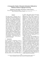
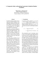
An example ADS architecture is depicted in
Figure 1, where we can see several components
trying to understand the user’s utterance and sev-
eral others trying to express the system’s re-
sponse. The system first attempts to convert spo-
ken input to text using the Automatic Speech
Recognition (ASR) component and then tries to
infer the meaning using the Natural Language Un-
derstanding (NLU) component. At the core lies
the Dialogue Manager (DM), a component re-
sponsible for understanding what the user’s utter-
ance means and deciding which action to take that
will lead to achieving his / her goals. The DM
may also take into account contextual information
22

Figure 1: Example architecture of an ADS.
or historical data before making a decision. After
the system has decided what to say, it uses the
Referring Expression Generation (REG) compo-
nent to create appropriate referring expressions,
the Natural Language Generation (NLG) compo-
nent to create the textual form of the output and
last, the Text To Speech (TTS) component to con-
vert the text to spoken output.
Trying to make ADS as human-like as possi-
ble researchers have focused on techniques that
achieve adaptation, i.e. adjust to the current user’s
personality, behaviour, mood, needs and to the
environment in general. Examples include adap-
tive or trainable NLG (Rieser and Lemon, 2009),
where the authors formulate their problem as a
statistical planning problem and use RL to find
a policy according to which the system will de-
cide how to present information. Another exam-
ple is adaptive REG (Janarthanam and Lemon,
2009), where the authors again use RL to choose
one of three strategies (jargon, tutorial, descrip-
tive) according to the user’s expertise level. An
example of adaptive TTS is the work of Boidin
et al. (2009), where the authors propose a model
that sorts paraphrases with respect to predictions
of which sounds more natural. Jur
ˇ
c
´

ı
ˇ
cek et al.
(2010) propose a RL algorithm to optimize ADS
parameters in general. Last, many researchers
have used RL to achieve adaptive Dialogue Man-
agement (Pietquin and Hastie, 2011; Ga
ˇ
si
´
c et al.,
2010; Cuay
´
ahuitl et al., 2010).
As the reader may have noticed, the current
trend in training these components is the appli-
cation of RL techniques. RL is a well established
field of artificial intelligence and provides us with
robust frameworks that are able to deal with un-
certainty and can scale to real world problems.
One sub category of RL is Online RL where the
system can be trained on the fly, as it interacts
with its environment. These techniques have re-
cently begun to be applied to Dialogue Manage-
ment and in this paper we perform an extensive
evaluation of several standard and state of the art
Online RL techniques on a generic dialogue prob-
lem. Our experiments were conducted with user
simulations, with or without noise and using a
model that is able to alter the user’s needs at any

given point. We were thus able to see how well
each algorithm adapted to minor (noise / uncer-
tainty) or major (change in user needs) changes in
the environment.
In general, RL algorithms fall in two cate-
gories, planning and learning algorithms. Plan-
ning or model-based algorithms use training ex-
amples from previous interactions with the envi-
ronment as well as a model of the environment
that simulates interactions. Learning or model-
free algorithms only use training examples from
previous interactions with the environment and
that is the main difference of these two categories,
according to Sutton and Barto, (1998). The goal
of an RL algorithm is to learn a good policy (or
strategy) that dictates how the system should in-
teract with the environment. An algorithm then
can follow a specific policy (i.e. interact with
the environment in a specific, maybe predefined,
way) while searching for a good policy. This way
of learning is called “off policy” learning. The op-
posite is “on policy” learning, when the algorithm
follows the policy that it is trying to learn. This
will become clear in section 2.2 where we pro-
vide the basics of RL. Last, these algorithms can
be categorized as policy iteration or value itera-
tion algorithms, according to the way they evalu-
ate and train a policy.
Table 1 shows the algorithms we evaluated
along with some of their characteristics. We se-

lected representative algorithms for each category
and used the Dyna architecture (Sutton and Barto,
1998) to implement model based algorithms.
SARSA(λ) (Sutton and Barto, 1998), Q Learn-
ing (Watkins, 1989), Q(λ) (Watkins, 1989; Peng
and Williams, 1996) and AC-QV (Wiering and
Van Hasselt, 2009) are well established RL al-
gorithms, proven to work and simple to imple-
ment. A serious disadvantage though is the fact
that they do not scale well (assuming we have
23
enough memory), as also supported by our results
in section 5. Least Squares SARSA(λ) (Chen and
Wei, 2008) is a variation of SARSA(λ) that uses
the least squares method to find the optimal pol-
icy. Incremental Actor Critic (IAC) (Bhatnagar
et al., 2007) and Natural Actor Critic (NAC) (Pe-
ters et al., 2005) are actor - critic algorithms that
follow the expected rewards gradient and the nat-
ural or Fisher Information gradient respectively
(Szepesv
´
ari, 2010).
An important attribute of many learning algo-
rithms is function approximation which allows
them to scale to real world problems. Function
approximation attempts to approximate a target
function by selecting from a class of functions
that closely resembles the target. Care must be
taken however, when applying this method, be-

cause many RL algorithms are not guaranteed to
converge when using function approximation. On
the other hand, policy gradient algorithms (algo-
rithms that perform gradient ascend/descend on
a performance surface), such as NAC or Natural
Actor Belief Critic (Jur
ˇ
c
´
ı
ˇ
cek et al., 2010) have
good guarantees for convergence, even if we use
function approximation (Bhatnagar et al., 2007).
Algorithm Model Policy Iteration
SARSA(λ) No On Value
LS-SARSA(λ) No On Policy
Q Learning No Off Value
Q(λ) No Off Value
Actor Critic - QV No On Policy
IAC No On Policy
NAC No On Policy
DynaSARSA(λ) Yes On Value
DynaQ Yes Off Value
DynaQ(λ) Yes Off Value
DynaAC-QV Yes On Policy
Table 1: Online RL algorithms used in our
evaluation.
While there is a significant amount of work in
evaluating RL algorithms, this is the first attempt,

to the best of our knowledge, to evaluate online
learning RL algorithms on the dialogue manage-
ment problem, in the presence of uncertainty and
changes in the environment.
Atkeson and Santamaria (1997) evaluate model
based and model free algorithms on the single
pendulum swingup problem but their algorithms
are not the ones we have selected and the prob-
lem on which they were evaluated differs from
ours in many ways. Ross et al. (2008) com-
pare many online planning algorithms for solving
Partially Observable Markov Decision Processes
(POMDP). It is a comprehensive study but not di-
rectly related to ours, as we model our problem
with Markov Decision Processes (MDP) and eval-
uate model-based and model-free algorithms on a
specific task.
In the next section we provide some back-
ground knowledge on MDPs and RL techniques,
in section 3 we present our proposed formulation
of the slot filling dialogue problem, in section 4
we describe our experimental setup and results, in
section 5 we discuss those results and in section 6
we conclude this study.
2 Background
In order to fully understand the concepts dis-
cussed in this work we will briefly introduce MDP
and RL and explain how these techniques can be
applied to the dialogue policy learning problem.
2.1 Markov Decision Process

A MDP is defined as a triplet M = {X, A, P },
where X is a non empty set of states, A is a non
empty set of actions and P is a transition probabil-
ity kernel that assigns probability measures over
X × R for each state-action pair (x, a) ∈ X × A.
We can also define the state transition probabil-
ity kernel P
t
that for each triplet (x
1
, a, x
2
) ∈
X × A × X would give us the probability of
moving from state x
1
to state x
2
by taking action
a. Each transition from a state to another is as-
sociated with an immediate reward, the expected
value of which is called the reward function and
is defined as R(x, a) = E[r(x, a)], where r(x, a)
is the immediate reward the system receives after
taking action a (Szepesv
´
ari, 2010). An episodic
MDP is defined as an MDP with terminal states,
X
t+s

= x, ∀s > 1. We consider an episode over
when a terminal state is reached.
2.2 Reinforcement Learning
Motivation to use RL in the dialogue problem
came from the fact that it can easily tackle some
of the challenges that arise when implementing
dialogue systems. One of those, for example, is
error recovery. Hand crafted error recovery does
not scale at all so we need an automated process
to learn error-recovery strategies. More than this
we can automatically learn near optimal dialogue
24
policies and thus maximize user satisfaction. An-
other benefit of RL is that it can be trained using
either real or simulated users and continue to learn
and adapt with each interaction (in the case of on-
line learning). To use RL we need to model the
dialogue system using MDPs, POMDPs or Semi
Markov Desicion Processes (SMDP). POMDPs
take uncertainty into account and model each state
with a distribution that represents our belief that
the system is in a specific state. SMDPs add tem-
poral abstraction to the model and allow for time
consuming operations. We, however, do not deal
with either of those in an attempt to keep the prob-
lem simple and focus on the task of comparing the
algorithms.
More formally, RL tries to maximize an objec-
tive function by learning how to control the ac-
tions of a system. A system in this setting is typ-

ically formulated as an MDP. As we discussed in
section 2.1 for every MDP we can define a pol-
icy π, which is a mapping from states x ∈ X and
actions α ∈ A to a distribution π(x, α) that repre-
sents the probability of taking action α when the
system is in state x. This policy dictates the be-
haviour of the system. To estimate how good a
policy is we define the value function V :
V
π
(x) = E[
∞

t=0
γ
t
R
t+1
|x
0
= x], x ∈ X (1)
which gives us the expected cumulative rewards
when beginning from state x and following policy
π, discounted by a factor γ ∈ [0, 1] that models
the importance of future rewards. We define the
return of a policy π as:
J
π
=
∞


t=0
γ
t
R
t
(x
t
, π(x
t
)) (2)
A policy π is optimal if J
π
(x) = V
π
(x), ∀x ∈
X. We can also define the action-value function
Q:
Q
π
(x, α) = E[
∞

t=0
γ
t
R
t+1
|x
0

= x, a
0
= α] (3)
where x ∈ X, α ∈ A, which gives us the ex-
pected cumulative discounted rewards when be-
ginning from state x and taking action α, again
following policy π. Note that V
max
=
r
max
1−γ
,
where R(x) ∈ [r
min
, r
max
].
The goal of RL therefore is to find the optimal
policy, which maximizes either of these functions
(Szepesv
´
ari, 2010).
3 Slot Filling Problem
We formulated the problem as a generic slot fill-
ing ADS, represented as an MDP. This model has
been proposed in (Papangelis et al., 2012), and we
extend it here to account for uncertainty. Formally
the problem is defined as: S =< s
0

, , s
N
>∈
M, M = M
0
× M
1
× ×M
N
, M
i
= {1, , T
i
},
where S are the N slots to be filled, each slot s
i
can take values from M
i
and T
i
is the number of
available values slot s
i
can be filled with. Dia-
logue state is also defined as a vector d ∈ M ,
where each dimension corresponds to a slot and
its value corresponds to the slot’s value. We call
the set of all possible dialogue states D. System
actions A ∈ {1, , |S|} are defined as requests
for slots to be filled and a

i
requests slot s
i
. At
each dialogue state d
i
we define a set of available
actions ˜a
i
⊂ A. A user query q ⊂ S is defined
as the slots that need to be filled so that the sys-
tem will be able to accurately provide an answer.
We assume action a
N
always means Give Answer.
The reward function is defined as:
R(d, a) =





−1, if a = a
N
−100, if a = a
N
, ∃q
i
|q
i

= ∅
0, if a = a
N
, ¬∃q
i
|q
i
= ∅
(4)
Thus, the optimal reward for each problem is −|q|
since |q| < |S|.
Available actions for every state can be mod-
elled as a matrix
˜
A ∈ {0, 1}
|D|×|A|
, where:
˜
A
ij
=

1, if a
j
∈ ˜a
i
0, if a
j
∈ ˜a
i

(5)
When designing
˜
A one must keep in mind that
the optimal solution depends on
˜
A’s structure
and must take care not to create an unsolvable
problem, i.e. a disconnected MDP. This can be
avoided by making sure that each action is avail-
able at some state and that each state has at least
one available action. We should now define the
necessary conditions for the slot filling problem
to be solvable and the optimal reward be as de-
fined before:
∃˜α
ij
= 1, 1 ≤ i < |D|, ∀j (6)
25
∃˜α
ij
= 1, 1 < j < |A|, ∀i (7)
Note that j > 1 since d
1
is our starting state. We
also allow Give Answer (which is a
N
) to be avail-
able from any state:
˜

A
i,N
= 1, 1 ≤ i ≤ |D| (8)
We define available action density to be the ra-
tio of 1s over the number of elements of
˜
A:
Density =
|{(i, j)|
˜
A
ij
= 1}|
|D| × |A|
We can now incorporate uncertainty in our
model. Rather than allowing deterministic transi-
tions from a state to another we define a distribu-
tion P
t
(d
j
|d
i
, a
m
) which models the probability
by which the system will go from state d
i
to d
j

when taking action a
m
. Consequently, when the
system takes action a
m
from state d
i
, it transits to
state d
k
with probability:
P
t
(d
k
|d
i
, a
m
) =



P
t
(d
j
|d
i
, a

m
), k = j
1−P
t
(d
j
|d
i
,a
m
)
|D|−1
, k = j
(9)
assuming that under no noise conditions action
a
m
would move the system from state d
i
to state
d
j
. The probability of not transiting to state d
j
is uniformly distributed among all other states.
P
t
(d
j
|d

i
, a
m
) is updated after each episode with
a small additive noise ν, mainly to model unde-
sirable or unforeseen effects of actions. Another
distribution, P
c
(s
j
= 1) ∈ [0, 1], models our con-
fidence level that slot s
j
is filled:
s
j
=

1, P
c
(s
j
= 1) ≥ 0.5
0, P
c
(s
j
= 1) < 0.5
(10)
In our evaluation P

c
(s
j
) is a random number be-
tween [1 − , 1] where  models the level of un-
certainty. Last, we can slightly alter
˜
A after each
episode to model changes or faults in the avail-
able actions for each state, but we did not in our
experiments.
The algorithms selected for this evaluation are
then called to solve this problem online and find
an optimal policy π

that will yield the highest
possible reward.
Algorithm α β γ λ
SARSA(λ) 0.95 - 0.55 0.4
LS-SARSA(λ) 0.95 - 0.55 0.4
Q Learning 0.8 - 0.8 -
Q(λ) 0.8 - 0.8 0.05
Actor Critic - QV 0.9 0.25 0.75 -
IAC 0.9 0.25 0.75 -
NAC 0.9 0.25 0.75 -
DynaSARSA(λ) 0.95 - 0.25 0.25
DynaQ 0.8 - 0.4 -
DynaQ(λ) 0.8 - 0.4 0.05
DynaAC-QV 0.9 0.05 0.75 -
Table 2: Optimized parameter values.

4 Experimental Setup
Our main goal was to evaluate how each algo-
rithm behaves in the following situations:
• The system needs to adapt to a noise free en-
vironment.
• The system needs to adapt to a noisy envi-
ronment.
• There is a change in the environment and the
system needs to adapt.
To ensure each algorithm performed to the best
of its capabilities we tuned each one’s parameters
in an exhaustive manner. Table 2 shows the pa-
rameter values selected for each algorithm. The
parameter  in -greedy strategies was set to 0.01
and model-based algorithms trained their model
for 15 iterations after each interaction with the
environment. Learning rates α and β and explo-
ration parameter  decayed as the episodes pro-
gressed to allow better stability.
At each episode the algorithms need enough it-
erations to explore the state space. At the initial
stages of learning, though, it is possible that some
algorithms fall into loops and require a very large
number of iterations before reaching a terminal
state. It would not hurt then if we bound the num-
ber of iterations to a reasonable limit, provided it
allows enough “negative” rewards to be accumu-
lated when following a “bad” direction. In our
evaluation the algorithms were allowed 2|D| iter-
ations, ensuring enough steps for exploration but

not allowing “bad” directions to be followed for
too long.
To assess each algorithm’s performance and
convergence speed, we run each algorithm 100
26
times on a slot filling problem with 6 slots, 6 ac-
tions and 300 episodes. The average reward over
a high number of episodes indicates how stable
each algorithm is after convergence. User query q
was set to be {s
1
, , s
5
} and there was no noise
in the environment, meaning that the action of
querying a slot deterministically gets the system
into a state where that slot is filled. This can be
formulated as: P
t
(d
j
|d
i
, a
m
) = 1, P
c
(s
j
) = 1∀j,

ν = 0 and
˜
A
i,j
= 1, ∀i, j.
To evaluate the algorithms’ performance in
the presence of uncertainty we run each for 100
times, on the same slot filling problem but with
P
t
(d
j
|d
i
, a
m
) ∈ [1 − , 1], with varying  and
available action density values. At each run, each
algorithm was evaluated using the same transition
probabilities and available actions. To assess how
the algorithms respond to environmental changes
we conducted a similar but noise free experiment,
where after a certain number of episodes the query
q was changed. Remember that q models the re-
quired information for the system to be able to an-
swer with some degree of certainty, so changing q
corresponds to requiring different slots to be filled
by the user. For this experiment we randomly gen-
erated two queries of approximately 65% of the
number of slots. The algorithms then needed to

learn a policy for the first query and then adapt
to the second, when the change occurs. This
could, for example, model scenarios where hotel
booking becomes unavailable or some airports are
closed, in a travel planning ADS. Last, we evalu-
ated each algorithm’s scalability, by running each
for 100 times on various slot filling problems, be-
ginning with a problem with 4 slots and 4 actions
up to a problem with 8 slots and 8 actions. We
measured the return averaged over the 100 runs
each algorithm achieved.
Despite many notable efforts, a standardized
evaluation framework for ADS or DS is still con-
sidered an open question by the research commu-
nity. The work in (Pietquin and Hastie, 2011)
provides a very good survey of current techniques
that evaluate several aspects of Dialogue Systems.
When RL is applied, researchers typically use
the reward function as a metric of performance.
This will be our evaluation metric as well, since
it is common across all algorithms. As defined
in section 2.3, it penalizes attempts to answer the
user’s query with incomplete information as well
as lengthy dialogues.
Algorithm Average Reward
SARSA(λ) -10.5967
LS-SARSA(λ) -14.3439
Q Learning -14.8888
Q(λ) -63.7588
Actor Critic - QV -15.9245

IAC -10.5000
NAC -5.8273
DynaSARSA(λ) -11.9758
DynaQ -14.7270
DynaQ(λ) -17.1964
DynaAC-QV -58.4576
Table 3: Average Total Reward without noise.
As mentioned earlier in the text we opted for
user simulations for our evaluation experiments
instead of real users. This method has a number of
advantages, for example the fact that we can very
quickly generate huge numbers of training exam-
ples. One might suggest that since the system is
targeted to real users it might not perform as well
when trained using simulations. However, as can
be seen from our results, there are online algo-
rithms, such as NAC or SARSA(λ), that can adapt
well to environmental changes, so it is reasonable
to expect such a system to adapt to a real user even
if trained using simulations. We can now present
the results of our evaluation, as described above
and in the next section we will provide insight on
the algorithms’ behaviour on each experiment.
Alg. E1 E2 E3 E4
S(λ) -7.998 -13.94 -23.68 -30.01
LSS -9.385 -12.34 -25.67 -32.33
Q -6.492 -15.71 -23.36 -30.56
Q(λ) -22.44 -23.27 -27.04 -29.37
AC -8.648 -17.91 -32.14 -38.46
IAC -6.680 -18.58 -33.60 -35.39

NAC -3.090 -9.142 -19.46 -21.33
DS(λ) -8.108 -15.61 -38.22 -41.90
DQ -6.390 -13.04 -23.64 -28.69
DQ(λ) -16.04 -17.33 -39.20 -38.42
DAC -28.39 -32.25 -44.26 -45.01
Table 4: Average Total Reward with noise.
4.1 Average reward without noise
Table 3 shows the average total reward each al-
gorithm achieved (i.e. the average of the sum of
rewards for each episode), over 100 runs, each
run consisting of 300 episodes. The problem had
6 slots, 6 actions, a query q = {s
1
, , s
5
} and
no noise. In this scenario the algorithms need to
learn to request each slot only once and give the
27
answer when all slots are filled. The optimal re-
ward in this case was −5. Remember that during
the early stages of training the algorithms receive
suboptimal rewards until they converge to the op-
timal policy that yields J
π
∗
= −5. The sum of re-
wards an algorithm received for each episode then
can give us a rough idea of how quickly it con-
verged and how stable it is. Clearly NAC outper-

forms all other algorithms with an average reward
of −5.8273 showing it converges early and is sta-
ble from then on. Note that the differences in per-
formance are statistically significant except be-
tween LS-SARSA(λ), DynaSARSA(λ) and Dy-
naQ Learning.
4.2 Average reward with noise
Table 4 shows results from four similar exper-
iments (E1, E2, E3 and E4), with 4 slots, 4
actions, q = {s
1
, s
2
, s
3
} and 100 episodes
but in the presence of noise. For E1 we set
P
t
(d
j
|d
i
, a
m
) = 1 and Density to 1, for E2 we
set P
t
(d
j

|d
i
, a
m
) = 0.8 and Density to 0.95, for
E3 we set P
t
(d
j
|d
i
, a
m
) = 0.6 and Density to
0.9 and for E4 we set P
t
(d
j
|d
i
, a
m
) = 0.4 and
Density to 0.8. After each episode we added a
small noise ν ∈ [−0.05, 0.05] to P
t
(·). Remem-
ber that each algorithm run for 2|D| iterations
(32 in this case) for each episode, so an aver-
age lower than −32 indicates slow convergence

or even that the algorithm oscillates. In E1, since
there are few slots and no uncertainty, most algo-
rithms, except for IAC, NAC and Q(λ) converge
quickly and have statistically insignificant differ-
ences with each other. In E2 we have less pairs
with statistically insignificant differences, and in
E3 and E4 we only have the ones mentioned in
the previous section. As we can see, NAC han-
dles uncertainty better, by a considerable margin,
than the rest algorithms. Note here that Q(λ) con-
verges late while Q Learning, Dyna Q Learning,
SARSA(λ) AC-QV and Dyna SARSA(λ) oscil-
late a lot in the presence of noise. The optimal
reward is −3, so it is evident that most algorithms
cannot handle uncertainty well.
4.3 Response to change
In this experiment we let each algorithm run for
500 episodes in a problem with 6 slots and 6
actions. We generated two queries, q
1
and q
2
,
consisting of 4 slots each, and begun the algo-
rithms with q
1
. After 300 episodes the query
was changed to q
2
and the algorithms were al-

lowed another 200 episodes to converge. Table
5 shows the episode at which, on average, each
algorithm converged after the change (after the
300
th
episode). Note here that the learning rates
α and β were reset at the point of change. Differ-
ences in performance, with respect to the average
reward collected during this experiment are statis-
tically significant, except between SARSA(λ), Q
Learning and DynaQ(λ). We can see that NAC
converges only after 3 episodes on average, with
IAC converging after 4. All other algorithms re-
quire many more episodes, from about 38 to 134.
Algorithm Episode
SARSA(λ) 360.5
LS-SARSA(λ) 337.6
Q Learning 362.8
Q(λ) 342.5
Actor Critic - QV 348.7
IAC 304.1
NAC 302.9
DynaSARSA(λ) 402.6
DynaQ 380.2
DynaQ(λ) 384.6
DynaAC-QV 433.3
Table 5: Average number of episodes required
for convergence after the change.
4.4 Convergence Speed
To assess the algorithms’ convergence speed we

run each algorithm 100 times for problems of “di-
mension” 4 to 8 (i.e. 4 slots and 4 actions, 5 slots
and 5 actions and so on). We then marked the
episode at which each algorithm had converged
and averaged it over the 100 runs. Table 6 shows
the results. It is important to note here that LS-
SARSA, IAC and NAC use function approxima-
tion while the rest algorithms do not. We, how-
ever, assume that we have enough memory for
problems up to 8 slots and 8 actions and are only
interested in how many episodes it takes each
algorithm to converge, on average. The results
show how scalable the algorithms are with respect
to computational power.
We can see that after dimension 7 many algo-
rithms require much more episodes in order to
converge. LS-SARSA(λ), IAC and NAC once
again seem to behave better than the others, re-
quiring only a few more episodes as the prob-
lem dimension increases. Note here however that
these algorithms take much more absolute time to
28
converge compared to simpler algorithms (eg Q
Learning) who might require more episodes but
each episode is completed faster.
Algorithm 4 5 6 7 8
S(λ) 5 23 29 42 101
LSS(λ) 10 22 27 38 51
Q 11 29 47 212 816
Q(λ) 5 12 29 55 96

AC 12 21 42 122 520
IAC 7 14 29 32 39
NAC 5 9 17 23 28
DS(λ) 5 11 22 35 217
DQ 15 22 60 186 669
DQ(λ) 9 13 55 72 128
DAC 13 32 57 208 738
Table 6: Average number of episodes required
for convergence on various problem dimensions.
5 Discussion
SARSA(λ) performed almost equally to IAC
at the experiment with deterministic transitions
but did not react well to the change in q. As
we can see in Table 6, SARSA(λ) generally con-
verges at around episode 29 for a problem with
6 slots and 6 actions, therefore the 61 episodes it
takes it to adapt to change are somewhat many.
This could be due to the fact that SARSA(λ) uses
eligibility traces which means that past state - ac-
tion pairs still contribute to the updates, so even if
the learning rate α is reset immediately after the
change to allow faster convergence, it seems not
enough. It might be possible though to come up
with a strategy and deal with this type of situa-
tion, for example zero out all traces as well as re-
setting α. SARSA(λ) performs above average in
the presence of noise in this particular problem.
LS-SARSA(λ) practically is SARSA(λ) with
function approximation. While this gives the ad-
vantage of requiring less memory, it converges a

little slower than SARSA(λ) in the presence of
noise or in noise free environments and it needs
more episodes to converge as the size of the prob-
lem grows. It does, however, react better to
changes in the user’s goals, since it requires 38
episodes to converge after the change, compared
to 27 it normally needs as we can see in Table 6.
Q Learning exhibits similar behaviour with
the only difference that it converges a little later.
Again it takes many episodes to converge after the
change in the environment (compared to the 47
that it needs initially). This could be explained by
the fact that Q Learning only updates one row of
Q(x, a) at each iteration, thus needing more itera-
tions for Q(x, a) to reflect expected rewards in the
new environment. Like SARSA(λ), Q Learning is
able to deal with uncertainty well enough on the
dialogue task in the given time, but does not scale
well.
Q(λ) , quite opposite from SARSA(λ) and Q
Learning, is the slowest to initially converge, but
handles changes in the environment much better.
In Q(λ) the update of Q(x, a) is (very roughly)
based on the difference of Q(x, a

) − Q(x, a
∗
)
where a
∗

is the best possible action the algo-
rithm can take, whereas in SARSA(λ) the update
is (again roughly) based on Q(x, a

) − Q(x, a).
Also, in Q(λ) eligibility traces become zero if the
selected action is not the best possible. These two
reasons help obsolete information in Q(x, a) be
quickly updated. While it performs worse in the
presence of uncertainty, the average reward does
not drop as steeply as for the rest algorithms.
AC-QV converges better than average, com-
pared to the other algorithms, and seems to cope
well with changes in the environment. While
it needs 42 episodes, on average, to converge
for a problem of 6 slots and 6 actions, it only
needs around 49 episodes to converge again af-
ter a change. Unlike SARSA(λ) and Q(λ) it does
not have eligibility traces to delay the update of
Q(x, a) (or P (x, a) for Preferences in this case,
see (Wiering and Van Hasselt, 2009)) while it also
keeps track of V (x). The updates are then based
on the difference of P (x, a) and V (x) which,
from our results, seems to make this algorithm be-
have better in a dynamic environment. AC-QV
also cannot cope with uncertainty very well on
this problem.
IAC is an actor - critic algorithm that fol-
lows the gradient of cumulative discounted re-
wards ∇J

π
. It always performs slightly worse
than NAC but in a consistent way, except in the
experiments with noise. It only requires approx-
imately 4 episodes to converge after a change
but cannot handle noise as well as other algo-
rithms. This can be in part explained by the
policy gradient theorem (Sutton et al., 2000) ac-
cording to which changes in the policy do not
29
affect the distribution of state the system visits
(IAC and NAC perform gradient ascend in the
space of policies rather than in parameter space
(Szepesv
´
ari, 2010)). Policy gradient methods in
general seem to converge rapidly, as supported by
results of Sutton et al. (2000) or Konda and Tsit-
siklis (2001) for example.
NAC , as expected, performs better than any
other algorithm in all settings. It not only con-
verges in very few episodes but is also very robust
to noise and changes in the environment. Follow-
ing the natural gradient has proven to be much
more efficient than simply using the gradient of
the expected rewards. There are many positive
examples of NAC performance (or following the
natural gradient in general), such as (Bagnell and
Schneider, 2003; Peters et al., 2005) and this work
is one of them.

Dyna Algorithms except for Dyna
SARSA(λ), seem to perform worse than av-
erage on the deterministic problem. In the
presence of changes, none of them seems to
perform very well. These algorithms use a
model of the environment to update Q(x, a) or
P (x, a), meaning that after each interaction with
the environment they perform several iterations
using simulated triplets (x, a, r). In the presence
of changes this results in obsolete information
being reused again and again until sufficient real
interactions with the environment occur and the
model is updated as well. This is possibly the
main reason why each Dyna algorithm requires
more episodes after the change than its corre-
sponding learning algorithm. Dyna Q Learning
only updates a single entry of Q(x, a) at each
simulated iteration, which could explain why
noise does not corrupt Q(x, a) too much and
why this algorithm performs well in the presence
of uncertainty. Noise in this case is added at a
single entry of Q(x, a), rather than to the whole
matrix, at each iteration. Dyna SARSA(λ) and
Dyna Q(λ) handle noise slightly better than Dyna
AC-QV.
6 Concluding Remarks
NAC proved to be the best algorithm in our eval-
uation. It is, however, much more complex to im-
plement and run and thus each episode takes more
(absolute) time to complete. One might suggest

then that a lighter algorithm such as SARSA(λ)
will have the opportunity to run more iterations
in the same absolute time. One should definitely
take this into account when designing a real world
system, when timely responses are necessary and
resources are limited as, for example, in a mobile
system. Note that SARSA(λ), Q-Learning, Q(λ)
and AC-QV are significantly faster than the rest
algorithms.
On the other hand, all algorithms except for
NAC, IAC and LS-SARSA have the major draw-
back of the size of the table representing Q(x, a)
or P (x, a) that is needed to store state-action val-
ues. This is a disadvantage that practically pro-
hibits the use of these algorithms in high dimen-
sional or continuous problems. Function approxi-
mation might alleviate this problem, according to
Bertsekas (2007), if we reformulate the problem
and reduce control space while increasing state
space. In such a setting function approximation
performs well, while in general it cannot deal with
large control spaces. It becomes very expensive
as computation cost grows exponentially on the
size of the lookahead horizon. Also, according to
Sutton and Barto (1998) and Sutton et al. (2000),
better convergence guarantees exist for online al-
gorithms when combined with function approx-
imation or for policy gradient methods (such as
IAC or NAC) in general. Finally, one must take
great care when selecting features to approximate

Q(x, a) or V (x) as they are important to con-
vergence and speed of the algorithm (Allen and
Fritzsche, 2011; Bertsekas, 2007).
To summarize, NAC outperforms the other al-
gorithms in every experiment we conducted. It
does require a lot of computational power though
and might not be suitable if it is limited. On
the other hand, SARSA(λ) or Q Learning per-
form well enough while requiring less computa-
tional power but a lot more memory space. The
researcher / developer then must make his / her
choice between them taking into account such
practical limitations.
As future work we plan to implement these al-
gorithms on the Olympus / RavenClaw (Bohus
and Rudnicky, 2009) platform, using the results
of this work as a guide. Our aim will be to cre-
ate a hybrid state of the art ADS that will com-
bine advantages of existing state of the art tech-
niques. Moreover we plan to install our system
on a robotic platform and conduct real user trials.
30
References
Allen, M., Fritzsche, P., 2011, Reinforcement Learn-
ing with Adaptive Kanerva Encoding for Xpilot
Game AI, Annual Congress on Evolutionary Com-
putation, pp 1521–1528.
Atkeson, C.G., Santamaria, J.C., 1997, A comparison
of direct and model-based reinforcement learning,
IEEE Robotics and Automation, pp 3557–3564.

Bagnell, J., Schneider, J., 2003, Covariant pol-
icy search, Proceedings of the Eighteenth Interna-
tional Joint Conference on Artificial Intelligence, pp
1019–1024.
Bertsekas D.P., 2007, Dynamic Programming and
Optimal Control, Athena Scientific, vol 2, 3rd edi-
tion.
Bhatnagar, S, Sutton, R.S., Ghavamzadeh, M., Lee,
M. 2007, Incremental Natural Actor-Critic Algo-
rithms, Neural Information Processing Systems, pp
105–112.
Bohus, D., Rudnicky, A.I., 2009, The RavenClaw di-
alog management framework: Architecture and sys-
tems, Computer Speech & Language, vol 23:3, pp
332-361.
Boidin, C., Rieser, V., Van Der Plas, L., Lemon, O.,
and Chevelu, J. 2009, Predicting how it sounds:
Re-ranking dialogue prompts based on TTS qual-
ity for adaptive Spoken Dialogue Systems, Pro-
ceedings of the Interspeech Special Session Ma-
chine Learning for Adaptivity in Spoken Dialogue,
pp 2487–2490.
Chen, S-L., Wei, Y-M. 2008, Least-Squares
SARSA(Lambda) Algorithms for Reinforcement
Learning, Natural Computation, 2008. ICNC ’08,
vol.2, pp 632–636.
Cuay
´
ahuitl, H., Renals, S., Lemon, O., Shimodaira,
H. 2010, Evaluation of a hierarchical reinforce-

ment learning spoken dialogue system, Computer
Speech & Language, Academic Press Ltd., vol 24:2,
pp 395–429.
Ga
ˇ
si
´
c, M., Jur
ˇ
c
´
ı
ˇ
cek, F., Keizer, S., Mairesse, F.
and Thomson, B., Yu, K. and Young, S, 2010,
Gaussian processes for fast policy optimisation of
POMDP-based dialogue managers, Proceedings
of the 11th Annual Meeting of the Special Interest
Group on Discourse and Dialogue, pp 201–204.
Geist, M., Pietquin, O., 2010, Kalman temporal
differences, Journal of Artificial Intelligence Re-
search, vol 39:1, pp 483–532.
Janarthanam, S., Lemon, O. 2009, A Two-Tier User
Simulation Model for Reinforcement Learning of
Adaptive Referring Expression Generation Policies,
SIGDIAL Conference’09, pp 120–123.
Jur
ˇ
c
´

ı
ˇ
cek, F., Thomson, B., Keizer, S., Mairesse, F.,
Ga
ˇ
si
´
c, M., Yu, K., Young, S 2010, Natural Belief-
Critic: A Reinforcement Algorithm for Parameter
Estimation in Statistical Spoken Dialogue Systems,
International Speech Communication Association,
vol 7, pp 1–26.
Konda, V.R., Tsitsiklis, J.N., 2001, Actor-Critic Al-
gorithms, SIAM Journal on Control and Optimiza-
tion, MIT Press, pp 1008–1014.
Konstantopoulos S., 2010, An Embodied Dialogue
System with Personality and Emotions, Proceedings
of the 2010 Workshop on Companionable Dialogue
Systems, ACL 2010, pp 3136.
Papangelis, A., Karkaletsis, V., Makedon, F., 2012,
Evaluation of Online Dialogue Policy Learning
Techniques, Proceedings of the 8th Conference on
Language Resources and Evaluation (LREC) 2012,
to appear.
Peng, J., Williams, R., 1996, Incremental multi-step
Q-Learning, Machine Learning pp 283–290.
Peters, J., Vijayakumar, S., Schaal, S. 2005, Natural
actor-critic , Machine Learning: ECML 2005, pp
280–291.
Pietquin, O., Hastie H. 2011, A survey on metrics for

the evaluation of user simulations, The Knowledge
Engineering Review, Cambridge University Press
(to appear).
Rieser, V., Lemon, O. 2009, Natural Language Gen-
eration as Planning Under Uncertainty for Spoken
Dialogue Systems, Proceedings of the 12th Confer-
ence of the European Chapter of the ACL (EACL
2009), pp 683–691.
Ross, S., Pineau, J., Paquet, S., Chaib-draa, B., 2008,
Online planning algorithms for POMDPs, Journal
of Artificial Intelligence Research, pp 663–704.
Sutton R.S., Barto, A.G., 1998, Reinforcement Learn-
ing: An Introduction, The MIT Press, Cambridge,
MA.
Sutton, R.S.,Mcallester, D., Singh, S., Mansour, Y.
2000, Policy gradient methods for reinforcement
learning with function approximation, In Advances
in Neural Information Processing Systems 12, pp
1057–1063.
Szepesv
´
ari, C., 2010, Algorithms for Reinforcement
Learning, Morgan & Claypool Publishers, Synthe-
sis Lectures on Artificial Intelligence and Machine
Learning, vol 4:1, pp 1–103.
Watkins C.J.C.H., 1989, Learning from delayed re-
wards, PhD Thesis, University of Cambridge, Eng-
land.
Wiering, M. A, Van Hasselt, H. 2009, The QV
family compared to other reinforcement learning

algorithms, IEEE Symposium on Adaptive Dy-
namic Programming and Reinforcement Learning,
pp 101–108.
Young S., Ga
ˇ
si
´
c, M., Keizer S., Mairesse, F., Schatz-
mann J., Thomson, B., Yu, K., 2010, The Hid-
den Information State model: A practical frame-
work for POMDP-based spoken dialogue manage-
ment, Computer Speech & Language, vol 24:2, pp
150–174.
31