mathematical model of movement of the observation and tracking head of an unmanned aerial vehicle performing ground target search and tracking

Hindawi Publishing Corporation
Journal of Applied Mathematics
Volume 2014, Article ID 934250, 11 pages
/>
Research Article
Mathematical Model of Movement of the Observation
and Tracking Head of an Unmanned Aerial Vehicle Performing
Ground Target Search and Tracking
Izabela Krzysztofik and Zbigniew Koruba
Department of Applied Computer Science and Armament Engineering, Faculty of Mechatronics and Machine Design,
Kielce University of Technology, 7 Tysiąclecia PP Street, 25-314 Kielce, Poland
Correspondence should be addressed to Izabela Krzysztofik;
Received 24 April 2014; Revised 31 July 2014; Accepted 2 August 2014; Published 8 September 2014
Academic Editor: Zheping Yan
Copyright © 2014 I. Krzysztofik and Z. Koruba. This is an open access article distributed under the Creative Commons Attribution
License, which permits unrestricted use, distribution, and reproduction in any medium, provided the original work is properly
cited.
The paper presents the kinematics of mutual movement of an unmanned aerial vehicle (UAV) and a ground target. The controlled
observation and tracking head (OTH) is a device responsible for observing the ground, searching for a ground target, and tracking
it. The preprogrammed movement of the UAV on the circle with the simultaneous movement of the head axis on Archimedes’ spiral
during searching for a ground target, both fixed (bunkers, rocket missiles launching positions, etc.) and movable (tanks, infantry
fighting vehicles, etc.), is considered. Dynamics of OTH during the performance of the above mentioned activities is examined.
Some research results are presented in a graphical form.

1. Introduction
Due to the advantages of unmanned aerial vehicles (UAV)
in relation to manned aircrafts, the multitask UAVs have
become the basic equipment of a modern army [1]. They
can carry out various tasks, such as aerial and radiolocation
reconnaissance, observation of the battlefield, radioelectronic
fight, adjustment of the artillery fire, target identification,

laser indication of the target, assessment of the effects of
striking other types of weapons, and imitation of air targets.
UAVs can also have a wide civilian application, for example,
observation and control of pipelines, electric tractions and
road traffic. Because of that, more than 250 UAV models are
developed and manufactured all over the world [2]. Many
scientific institutions are engaged in developing and identifying models of dynamics and flight control of UAVs. For
instance, papers [3, 4] present the comprehensive research
on modelling the dynamics of flight of K100 UAV and
Thunder Tiger Raptor 50 V2 Helicopter, respectively. Mathematical models of UAV with 6 degrees of freedom (6-DoF)

introduced on the basis of the Newton’s rules of dynamics
were presented, whereas [5] presents the methodology of
modelling the dynamics of UAV flight with the use of neural
networks. Paper [6] presents the mathematical model and the
experimental research on SUAVI. That vehicle can take off
and land vertically. The model was carried out with the use of
the Newton-Euler formalism. Moreover, the controllers for
controlling the height and stabilizing the vehicle’s location
have been developed. Paper [7] describes the problem of flight
dynamics of the UAV formation with the use of models with
3 and 6 degrees of freedom.
An operation of UAV during the completion of a task is
a complex process requiring comprehensive technical means
and systems. The control system of UAV is one of the most
important systems. Its task is to measure, evaluate, and
control flight parameters, as well as properly control the
flight and observation systems. Thanks to the use of complex
microprocessor systems, the comprehensive automation of
the mentioned processes is possible. Formerly, during the

completion of a mission it was necessary to maintain bilateral


2

Journal of Applied Mathematics
UAV
Observation and
tracking head (OTH)
C

Target observation
line (TOL)

Scanning of
ground surface

Target

H

T

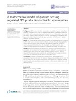
Figure 1: General view of the process of scanning the ground surface from UAV deck.

communications with the ground control point. In modern
UAVs, autonomy plays an important role during detecting
and tracking a ground target.
Paper [8] presents the model of the UAV autopilot and its
sensors in the Matlab-Simulink environment for simulation

research. Papers [9–11] pertain to planning and optimizing
the trajectory of movement of the vehicle. The aspects of
designing PID controllers for the systems of UAV flight
control have been discussed in papers [12, 13].
From the quoted review of the literature it appears that the
research mainly concentrates on UAV dynamics and control,
without the consideration of the model of movement of the
observation and tracking head (OTH) which is one of the
most significant elements of the unmanned aerial vehicle.
OTH is used for automatic searching for and tracking of
targets intended for destruction [14]. This paper presents the
mathematical model of kinematics of the movement of UAV,
the ground target, and the dynamics of the controlled head
located on the UAV deck. It needs to be emphasized that the
problem of modelling, examining the dynamics, and control
of such heads in the conditions of interferences from its base
(deck of the manoeuvring UAV) is still topical. The paper
examines this type of OTH with the built-in television and
thermographic cameras and the laser illuminator.

2. Model of Movement Kinematics of
UAV, OTH and Ground Target
General view of the process of searching for a target on the
surface of the ground by OTH from UAV deck is shown in
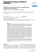
Figure 1, whereas the operation algorithm of OTH during
scanning the ground surface and tracking a target detected
on it is shown in Figure 2.

During the search for a ground target from UAV deck,
the axis of OTH should perform the desired movements and

circle strictly defined lines on the ground with the use of
its extension. The optical system of OTH, having a certain
viewing angle, may in this way encounter a light or infrared
signal emitted by the moving object. Therefore, one should
choose the kinematic parameters of mutual movement of
UAV deck and OTH in such a way that the likelihood of
detecting a target was the highest [15]. After locating a target,
OTH goes to the tracking mode; that is, from that moment
its axis has a specific location in space being pointed at the
target.
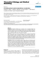
Figure 3 shows the kinematics of mutual movement of
the head axis and UAV during searching for a target on
the ground surface. Individual coordinate systems have the
following meaning:
𝑂𝑥𝑔 𝑦𝑔 𝑧𝑔 —Earth-fixed reference system,
𝐶𝑥𝑎 𝑦𝑎 𝑧𝑎 —coordinate system connected with target
observation line (TOL),
𝐶𝑥𝑐 𝑦𝑐 𝑧𝑐 —movable coordinate system connected with
UAV velocity vector.
The velocity of changing vector 𝑅⃗ in time, during searching for and tracking a target, is as follows:
𝑑𝑅⃗
= Π (𝑡𝑜 , 𝑡𝑑 ) ⋅ (𝑉𝑐⃗ − 𝑉ℎ⃗ )
𝑑𝑡

(1)

+ [Π (𝑡𝑑 , 𝑡𝑡 ) + Π (𝑡𝑡 , 𝑡𝑒 )] ⋅ (𝑉𝑐⃗ − 𝑉𝑡⃗ ) ,
where 𝑅⃗ is vector of the mutual distance of points 𝐶 and
𝐻 (during scanning the space) or points 𝐶 and 𝑇 (during

Journal of Applied Mathematics

3

Target

Autopilot
𝛿m , 𝛿n

Unmanned aerial
vehicle (UAV)

Control system
(CS)
pc∗

No
Yes

𝜓 h , 𝜗h

q c∗

Target observation line
(TOL)

rc∗

𝜀, 𝜎

Observation and
tracking head
(OTH)

𝜓 h , 𝜗h

Mex , Min

Pre-programmed

𝜓hr , 𝜗hr

control
p
p
Mex
, Min

Pre-programmed
movement
Generator
(searching
of target)

Tracking
movement
Generator
(tracking
of target)

Tracking
𝜀, 𝜎

control
t
t
Mex
, Min

No

Is target
detected?

Yes

Figure 2: Diagram of operation of OTH mounted on UAV deck.

tracking); 𝑉𝑐⃗ , 𝑉ℎ⃗ , 𝑉𝑡⃗ are vectors of the velocity of movement
of the centre of mass of UAV, of points 𝐻 and 𝑇, respectively; Π(𝑡𝑜 , 𝑡𝑑 ), Π(𝑡𝑑 , 𝑡𝑡 ), Π(𝑡𝑡 , 𝑡𝑒 ) are functions of rectangular
impulse; 𝑡𝑜 is the moment the scanning the ground is started;
𝑡𝑑 is the moment a target is detected; 𝑡𝑡 is the moment the
tracking the target is started; 𝑡𝑒 is the moment the scanning
process and tracking the target is finished.
We project the left side of (1) on the axes of the coordinate
system 𝐶𝑥𝑎 𝑦𝑎 𝑧𝑎 (Figure 3) connected with vector 𝑅.⃗ In the
result we get
󵄨
󵄨󵄨 ⃗

󵄨󵄨 𝑖𝑎
𝑗𝑎⃗
𝑘⃗ 𝑎 󵄨󵄨󵄨
󵄨󵄨
󵄨
⃗
󵄨
𝑑𝑅 𝑑𝑅 ⃗ 󵄨󵄨
󵄨
𝑖𝑎 + 󵄨󵄨𝜔𝑅𝑥𝑎 𝜔𝑅𝑦𝑎 𝜔𝑅𝑧𝑎 󵄨󵄨󵄨
=
󵄨󵄨
󵄨󵄨
𝑑𝑡
𝑑𝑡
󵄨
󵄨󵄨
󵄨󵄨 𝑅
0
0 󵄨󵄨󵄨

Next, we project the right side of (1) (i.e., velocities 𝑉𝑐⃗ , 𝑉ℎ⃗
and 𝑉𝑡⃗ ) on the axes of the system 𝐶𝑥𝑎 𝑦𝑎 𝑧𝑎 and get
𝑑𝑅
= Π (𝑡𝑜 , 𝑡𝑑 ) ⋅ (𝑉𝑐𝑥𝑎 − 𝑉ℎ𝑥𝑎 )
𝑑𝑡
+ [Π (𝑡𝑑 , 𝑡𝑡 ) + Π (𝑡𝑡 , 𝑡𝑒 )] ⋅ (𝑉𝑐𝑥𝑎 − 𝑉𝑡𝑥𝑎 ) ,
𝑅

𝑑𝜎

cos 𝜀 = Π (𝑡𝑜 , 𝑡𝑑 ) ⋅ (𝑉𝑐𝑦𝑎 − 𝑉ℎ𝑦𝑎 )
𝑑𝑡
+ [Π (𝑡𝑑 , 𝑡𝑡 ) + Π (𝑡𝑡 , 𝑡𝑒 )] ⋅ (𝑉𝑐𝑦𝑎 − 𝑉𝑡𝑦𝑎 ) ,
𝑅

(2)

𝑑𝑅
𝑑𝜎
𝑑𝜀
= 𝑖𝑎⃗
+ 𝑗𝑎⃗ 𝑅
cos 𝜀 − 𝑘⃗ 𝑎 𝑅 ,
𝑑𝑡
𝑑𝑡
𝑑𝑡
where 𝜔𝑅𝑥𝑎 , 𝜔𝑅𝑦𝑎 , 𝜔𝑅𝑧𝑎 are components of angular velocity of
TOL and 𝜎, 𝜀 are angles of deflection and inclination of vector
𝑅.⃗

(3)

𝑑𝜀
= Π (𝑡𝑜 , 𝑡𝑑 ) ⋅ (𝑉𝑐𝑧𝑎 − 𝑉ℎ𝑧𝑎 )
𝑑𝑡
+ [Π (𝑡𝑑 , 𝑡𝑡 ) + Π (𝑡𝑡 , 𝑡𝑒 )] ⋅ (𝑉𝑐𝑧𝑎 − 𝑉𝑡𝑧𝑎 ) .

Individual components of velocity vectors 𝑉𝑐⃗ , 𝑉ℎ⃗ and 𝑉𝑡⃗
in the system 𝐶𝑥𝑎 𝑦𝑎 𝑧𝑎 are as follows:
𝑉𝑐𝑥𝑎 = 𝑉𝑐 [cos 𝜀 cos 𝛾𝑐 cos (𝜎 − 𝜒𝑐 ) + sin 𝜀 sin 𝛾𝑐 ] ,

(4a)

𝑉𝑐𝑦𝑎 = − 𝑉𝑐 cos 𝛾𝑐 sin (𝜎 − 𝜒𝑐 ) ,

(4b)

𝑉𝑐𝑧𝑎 = 𝑉𝑐 [sin 𝜀 cos 𝛾𝑐 cos (𝜎 − 𝜒𝑐 ) − cos 𝜀 sin 𝛾𝑐 ] ,

(4c)


4

Journal of Applied Mathematics
The derivative of that expression in relation to time is as
follows:

zg

zc
→

𝜔c

za

𝑑𝜀
𝑑𝑟 𝑑𝑅
=

cos 𝜀 − 𝑅 sin 𝜀.
𝑑𝑡
𝑑𝑡
𝑑𝑡

UAV path

C

→

Vc
→

rc

xc

O󳰀

(9)

ya

Let us substitute (4a)–(6c) into (3). Next, taking into
account (7)–(9), (3) will have the following form:

yc

𝑑𝑟

= Π (𝑡𝑜 , 𝑡𝑑 ) [𝑉𝑐 cos (𝜎 − 𝜒𝑐𝑠 ) − 𝑉ℎ cos (𝜎 − 𝜒ℎ )]
𝑑𝑡

→

R

Hc

𝜓hr

+ Π (𝑡𝑑 , 𝑡𝑡 ) [𝑉𝑐 cos (𝜎 − 𝜒𝑐𝑑 ) − 𝑉𝑡 cos (𝜎 − 𝜒𝑡 )]

𝜗hr

+ Π (𝑡𝑡 , 𝑡𝑒 ) [𝑉𝑐 cos (𝜎 − 𝜒𝑐𝑡 ) − 𝑉𝑡 cos (𝜎 − 𝜒𝑡 )] ,

→

xg

Vt
𝜒t

T

Target path

(10)

C󳰀

ry

𝑠

rx

→

Vh
yg

Path of point H
O

𝑉 sin (𝜎 − 𝜒𝑐 ) − 𝑉ℎ sin (𝜎 − 𝜒ℎ )
𝑑𝜎
= Π (𝑡𝑜 , 𝑡𝑑 ) 𝑐
𝑑𝑡
𝑟

→

Rh

H

+ Π (𝑡𝑑 , 𝑡𝑡 ) ⋅

xa

Figure 3: Kinematics of mutual movement of the head axis and UAV
during scanning the ground surface.

𝑉ℎ𝑥𝑎 = 𝑉ℎ [cos 𝜀 cos 𝛾ℎ cos (𝜎 − 𝜒ℎ ) + sin 𝜀 sin 𝛾ℎ ] ,

(5a)

𝑉ℎ𝑦𝑎 = − 𝑉ℎ cos 𝛾ℎ sin (𝜎 − 𝜒ℎ ) ,

(5b)

𝑉ℎ𝑧𝑎 = 𝑉ℎ [sin 𝜀 cos 𝛾ℎ cos (𝜎 − 𝜒ℎ ) − cos 𝜀 sin 𝛾ℎ ] ,

(5c)

𝑉𝑡𝑥𝑎 = 𝑉𝑡 [cos 𝜀 cos 𝛾𝑡 cos (𝜎 − 𝜒𝑡 ) + sin 𝜀 sin 𝛾𝑡 ] ,

(6a)

𝑉𝑡𝑦𝑎 = − 𝑉𝑡 cos 𝛾𝑡 sin (𝜎 − 𝜒𝑡 ) ,

(6b)

𝑉𝑡𝑧𝑎 = 𝑉𝑡 [sin 𝜀 cos 𝛾𝑡 cos (𝜎 − 𝜒𝑡 ) − cos 𝜀 sin 𝛾𝑡 ] ,

(6c)

where 𝜒𝑐 , 𝛾𝑐 are UAV flight angles, 𝜒ℎ , 𝛾ℎ are angles of

deflection and inclination of velocity vector of point 𝐻, and
𝜒𝑡 , 𝛾𝑡 are angles of deflection and inclination of velocity vector
of point 𝑇.
For the simplification of reasoning, we assume that the
movement of UAV, during searching and tracking, is done on
a horizontal plane at a set altitude 𝐻𝑐 , whereas the target and
point 𝐻 move in the ground plane. Then, we can assume that
𝛾𝑐 = 0,

𝛾𝑡 = 0,

𝛾ℎ = 0.

(7)

+ Π (𝑡𝑡 , 𝑡𝑒 )

𝑉𝑐 sin (𝜎 − 𝜒𝑐𝑑 ) − 𝑉𝑡 sin (𝜎 − 𝜒𝑡 )

𝑉𝑐 sin (𝜎 −

𝑟
𝜒𝑐𝑡 )

(8)

(11)

where 𝑟 is mutual distance of points 𝐶 and 𝐻 (during
scanning) or 𝐶 and 𝑇 (during tracking); 𝜒𝑐𝑠 is angle of

deflection of UAV velocity vector during scanning the ground
by the head; 𝜒𝑐𝑑 is angle of deflection of UAV velocity vector
during the passage from preprogrammed flight to tracking
flight; and 𝜒𝑐𝑡 is angle of deflection of UAV velocity vector
during the flight tracking the detected target.
We demand that, at the moment of detecting the target,
UAV automatically is starting the passage to the flight
tracking the detected target; that is, it is moving at a set
constant distance from the target 𝑟𝑐0 = 𝑅𝑐0 cos 𝜀 = const (in a
horizontal plane at a constant altitude 𝐻𝑐 ).
If the mutual distance 𝑟 of points 𝐶 and 𝑇 is different from
𝑟𝑐0 then the angle of deflection of UAV velocity vector 𝜒𝑐 = 𝜒𝑐𝑑
changes in accordance with the relationship:
𝑑𝜒𝑐𝑑
𝑑𝜎
= 𝑎𝑐 ⋅ sign (𝑟𝑐0 − 𝑟)
,
𝑑𝑡
𝑑𝑡

(12)

where 𝑎𝑐 is the set constant of proportional navigation.
After the fulfillment of the condition 𝑟 = 𝑟𝑐0 the
programme of angle change 𝜒𝑐𝑡 can be determined from (10):

We mark that
𝑟 = 𝑅 cos 𝜀

− 𝑉𝑡 sin (𝜎 − 𝜒𝑡 )

,
𝑟

𝜒𝑐𝑡 = 𝜎 − arc cos [

𝑉𝑡
cos (𝜎 − 𝜒𝑡 )] .
𝑉𝑐

(13)


Journal of Applied Mathematics

5

The path of UAV flight during scanning and tracking is as
follows :
𝑑𝑟𝑐
= Π (𝑡𝑜 , 𝑡𝑑 ) 𝑉𝑐 cos (𝜃𝑐 − 𝜒𝑐𝑠 ) + Π (𝑡𝑑 , 𝑡𝑡 ) 𝑉𝑐 cos (𝜃𝑐 − 𝜒𝑐𝑑 )
𝑑𝑡
+ Π (𝑡𝑡 , 𝑡𝑒 ) 𝑉𝑐 cos (𝜃𝑐 − 𝜒𝑐𝑡 ) ,
(14a)
𝑑𝜃𝑐
𝑉
𝑉
= Π (𝑡𝑜 , 𝑡𝑑 ) 𝑐 sin (𝜃𝑐 − 𝜒𝑐𝑠 ) + Π (𝑡𝑑 , 𝑡𝑡 ) 𝑐 sin (𝜃𝑐 − 𝜒𝑐𝑑 )
𝑑𝑡
𝑟𝑐
𝑟𝑐

+ Π (𝑡𝑡 , 𝑡𝑒 )

𝑉𝑐
sin (𝜃𝑐 − 𝜒𝑐𝑡 ) ,
𝑟𝑐

𝑟𝑐𝑥 = 𝑟𝑐 cos 𝜃𝑐 ,
𝑟𝑐𝑦 = 𝑟𝑐 sin 𝜃𝑐 ,

(14b)

(15)

where 𝑟𝑐 is vector of location of UAV mass centre (point 𝐶)
and 𝜃𝑐 is angle of deflection of vector 𝑟𝑐 .
Path of movement of point 𝐻 is as follows:
𝑑𝑅ℎ
= Π (𝑡𝑜 , 𝑡𝑑 ) 𝑉ℎ cos (𝜃ℎ − 𝜒ℎ ) ,
𝑑𝑡

(16a)

𝑑𝜃ℎ
= Π (𝑡𝑜 , 𝑡𝑑 ) 𝑉ℎ sin (𝜃ℎ − 𝜒ℎ ) ,
𝑑𝑡

(16b)

where
𝑟𝑥 = 𝑟 cos 𝜎,

𝑟𝑦 = 𝑟 sin 𝜎;

𝑑𝑟𝑥 𝑑𝑟
𝑑𝜎
=
cos 𝜎 − 𝑟
sin 𝜎;
𝑑𝑡
𝑑𝑡
𝑑𝑡
𝑑𝑟𝑦
𝑑𝑡

=

(21)

𝑑𝑟
𝑑𝜎
sin 𝜎 + 𝑟
cos 𝜎.
𝑑𝑡
𝑑𝑡

Values (20) are used for determining the preprogrammed
controls influencing the head.
2.1. Scanning the Ground Surface during UAV Flight on a
Circle. We assume that during scanning the set area of the
ground, UAV flight is at a constant altitude 𝐻𝑐 in a horizontal

plane on the circle of the set radius 𝑟𝑐 with constant velocity
𝑉𝑐 (Figure 3).
Then the preprogrammed UAV flight can be determined
from the following relationships:
𝑉𝑐 = 𝜔𝑐 ⋅ 𝑟𝑐 ,

𝜒𝑐 = 𝜔𝑐 𝑡.

(22)

At the same time, we control the head axis in such a way
that it drawn on the surface of the ground a curve in the shape
of Archimedean spiral with angular velocity
𝜔ℎ =

2𝜋𝑉ℎ
.
𝜌ℎ

(23)

where 𝑅ℎ is vector of location of point 𝐻 and 𝜃ℎ is angle of
deflection of vector 𝑅ℎ .
Path of movement of the target is as follows:

Velocity 𝑉ℎ is to be chosen in such a way that OTH
mounted on UAV deck could in the set time 𝑡𝑠 scan densely
enough the set surface of the area in the shape of a circle of
the radius 𝑅𝑠 .
If the angle of vision of the head’s optical system amounts

to 𝜙ℎ then lens coverage embraces the surface similar in shape
to a circle of the radius:

𝑑𝑅𝑡
= Π (𝑡𝑑 , 𝑡𝑒 ) 𝑉𝑡 cos (𝜃𝑡 − 𝜒𝑡 ) ,
𝑑𝑡

(18a)

1
𝜌ℎ = 𝐻𝑐 𝜙ℎ .
2

𝑑𝜃𝑡
= Π (𝑡𝑑 , 𝑡𝑒 ) 𝑉𝑡 sin (𝜃𝑡 − 𝜒𝑡 ) ,
𝑑𝑡

(18b)

𝑅ℎ𝑥 = 𝑅ℎ cos 𝜃ℎ ,
𝑅ℎ𝑦 = 𝑅ℎ sin 𝜃ℎ ,

𝑅𝑡𝑥 = 𝑅𝑡 cos 𝜃𝑡 ,
𝑅𝑡𝑦 = 𝑅𝑡 sin 𝜃𝑡 ,

(17)

(19)

where 𝑅𝑡 is vector of location of point 𝑇 and 𝜃𝑡 is angle of

deflection of vector 𝑅𝑡 .
̇ , 𝜓̇ of
Desired angles 𝜗ℎ𝑟 , 𝜓ℎ𝑟 and angular velocities 𝜗ℎ𝑟
ℎ𝑟
deflection of OTH axis can be determined from the following
relationships:
𝜗ℎ𝑟 = arc 𝑡𝑔

𝜓ℎ𝑟 = arc 𝑡𝑔

𝑟𝑥
,
𝐻𝑐

𝑑𝜗ℎ𝑟 𝐻𝑐 (𝑑𝑟𝑥 /𝑑𝑡)
,
=
2
𝑑𝑡
𝐻𝑐2 + (𝑟𝑥 )

𝑟𝑦

𝑑𝜓ℎ𝑟 𝐻𝑐 (𝑑𝑟𝑦 /𝑑𝑡)
,
=
2
𝑑𝑡
𝐻𝑐2 + (𝑟𝑦 )

𝐻𝑐

,

(20)

(24)

After detecting a target at the moment 𝑡𝑑 , UAV passes into
the tracking flight according to the relationship (12), while
the target is lit with a laser beam for the period of time 𝑡𝑙 .
Hence, the total time of the process of detecting, tracking, and
lighting the target amounts to 𝑡𝑒 = 𝑡𝑑 + 𝑡𝑙 .

3. The Model of Dynamics of the Controlled
Observation and Tracking Head
A spatial model of dynamics of the head presented in Figure 4
was adopted for the paper. OTH comprises two basic parts:
external frame and internal frame with camera. Movement
of the head is determined with the use of two angles: angle of
head deflection 𝜓ℎ and angle of head inclination 𝜗ℎ [16].
The following coordinate systems, shown in Figure 5,
have been introduced:
𝐶𝑥𝑑 𝑦𝑑 𝑧𝑑 —the movable system connected with the
UAV deck,


6

Journal of Applied Mathematics

𝜓h

Components of angular velocity of the internal frame of
the head are

Base

External
frame

𝜔𝑥ℎ = 𝜔𝑥ℎ1 cos 𝜗ℎ − 𝜔𝑧ℎ1 sin 𝜗ℎ ,

(26a)

𝜔𝑦ℎ = 𝜔𝑦ℎ1 + 𝜗ℎ̇ ,

(26b)

𝜔𝑧ℎ = 𝜔𝑥ℎ1 sin 𝜗ℎ + 𝜔𝑧ℎ1 cos 𝜗ℎ .

(26c)

Components of linear velocity of displacement of mass
centre of the external frame of the head are

𝜗h
Oh

𝑉𝑥ℎ1 = 𝑉𝑐 cos 𝜓ℎ ,

(27a)

𝑉𝑦ℎ1 = −𝑉𝑐 sin 𝜓ℎ ,

(27b)

𝑉𝑧ℎ1 = 0.

(27c)

Internal frame
with camera

Figure 4: General view of the observation and tracking head.

zd

zh

Components of linear velocity of displacement of mass
centre of the internal frame of the head are

zh1

𝜗h

𝑉𝑥ℎ = 𝑉𝑥ℎ1 cos 𝜗ℎ + 𝑙ℎ 𝜔𝑦ℎ1 sin 𝜗ℎ ,

(28a)

𝑉𝑦ℎ = 𝑉𝑦ℎ1 + 𝑙ℎ (𝜔𝑧ℎ1 + 𝜔𝑧ℎ ) ,

(28b)

𝑉𝑧ℎ = 𝑉𝑥ℎ1 sin 𝜗ℎ − 𝑙ℎ (𝜔𝑦ℎ1 cos 𝜗ℎ + 𝜔𝑦ℎ ) .

(28c)

→

𝜓̇ h

Using the second order Lagrange equations, the following
equations of the head movement have been derived:

→

C, Oh

𝜗̇ h
yh
𝜓h

𝜓h

xd

𝜗h

𝐽𝑧ℎ1

yh1

𝑑
𝑑
𝑑
𝜔 − 𝐽𝑥ℎ (𝜔𝑥ℎ sin 𝜗ℎ ) + 𝐽𝑧ℎ (𝜔𝑧ℎ cos 𝜗ℎ )
𝑑𝑡 𝑧ℎ1
𝑑𝑡
𝑑𝑡
+ 𝑚𝑟𝑤 𝑙ℎ

yd

𝑑
[𝑉 (1 + cos 𝜗ℎ )] − (𝐽𝑥ℎ1 − 𝐽𝑦ℎ1 ) 𝜔𝑥ℎ1 𝜔𝑦ℎ1
𝑑𝑡 𝑦ℎ

− 𝐽𝑥ℎ 𝜔𝑥ℎ 𝜔𝑦ℎ1 cos 𝜗ℎ + 𝐽𝑦ℎ 𝜔𝑦ℎ 𝜔𝑥ℎ1 − 𝐽𝑧ℎ 𝜔𝑧ℎ 𝜔𝑦ℎ1 sin 𝜗ℎ

xh1

+ 𝑚in 𝑙ℎ [𝑉𝑥ℎ 𝜔𝑥ℎ1 sin 𝜗ℎ − 𝑉𝑦ℎ 𝜔𝑦ℎ1 sin 𝜗ℎ

xh

Figure 5: Transformations of the coordinate systems.

−𝑉𝑧ℎ 𝜔𝑥ℎ1 (1 + cos 𝜗ℎ )]

+ 𝑚in 𝑙ℎ [𝑉𝑥ℎ1 (𝜔𝑧ℎ1 + 𝜔𝑧ℎ ) + 𝑉𝑦ℎ1 𝜔𝑦ℎ sin 𝜗ℎ ]

𝑂ℎ 𝑥ℎ1 𝑦ℎ1 𝑧ℎ1 —the movable system connected with
the external frame of the head,
𝑂ℎ 𝑥ℎ 𝑦ℎ 𝑧ℎ —the movable system connected with
internal the frame of the head (including camera).

𝑔
= 𝑀ex + 𝑀ex
− 𝑀𝑑ex ,

𝐽𝑦ℎ

𝑑
𝑑
𝜔𝑦ℎ − 𝑚in 𝑙ℎ 𝑉𝑧ℎ + (𝐽𝑥ℎ − 𝐽𝑧ℎ ) 𝜔𝑥ℎ 𝜔𝑧ℎ
𝑑𝑡
𝑑𝑡
𝑔

Components of angular velocity of the external frame of
the head are
𝜔𝑥ℎ1 = 𝑝𝑐∗ cos 𝜓ℎ + 𝑞𝑐∗ sin 𝜓ℎ ,

(25a)

𝜔𝑦ℎ1 = −𝑝𝑐∗ sin 𝜓ℎ + 𝑞𝑐∗ cos 𝜓ℎ ,

(25b)

𝜔𝑧ℎ1 = 𝜓̇ℎ + 𝑟𝑐∗ ,

(25c)

where 𝑝𝑐∗ , 𝑞𝑐∗ , 𝑟𝑐∗ are components of angular velocity of UAV.

− 𝑚in 𝑙ℎ [𝑉𝑦ℎ 𝜔𝑥ℎ − 𝑉𝑥ℎ 𝜔𝑦ℎ ] = 𝑀in + 𝑀in − 𝑀𝑑in ,
(29)
where 𝜓ℎ , 𝜗ℎ are angles of location of OTH axis in space;
𝑚in is the mass of internal frame with camera; 𝑙ℎ is the
distance of mass centre of internal frame (camera) from the
centre of movement; 𝐽𝑥ℎ1 , 𝐽𝑦ℎ1 , 𝐽𝑧ℎ1 are moments of inertia of
external frame; 𝐽𝑥ℎ , 𝐽𝑦ℎ , 𝐽𝑧ℎ are moments of inertia of internal
frame (with camera); 𝑀ex , 𝑀in are moments of controlling
forces influencing, respectively, external and internal frame;
𝑔
𝑔
, 𝑀in are moments of the force of gravity influencing
𝑀ex


Journal of Applied Mathematics

7
𝑔

𝑔
respectively: external and internal frame; 𝑀ex
= 0; 𝑀in =
𝑚in 𝑔𝑙ℎ cos 𝜗ℎ ; and 𝑀⃗ 𝑑ex , 𝑀⃗ 𝑑in are moments of friction forces

in the bearings of, respectively, external and internal frame.
We assume viscous friction:

𝑀𝑑ex = 𝜂ex 𝜓̇ℎ ;

𝑀𝑑in

= 𝜂in 𝜗ℎ̇ ,

(30)

where 𝜂ex is friction coefficient in suspension bearing of
external frame and 𝜂in is friction coefficient in suspension
bearing of internal frame.
Control moments 𝑀ex , 𝑀in of the head will be presented
as follows [17–19]:
𝑝
𝑡
𝑀ex = Π (𝑡𝑜 , 𝑡𝑑 ) ⋅ 𝑀ex
(𝑡) + Π (𝑡𝑡 , 𝑡𝑒 ) ⋅ 𝑀ex
(𝑡) ,

𝑀in = Π (𝑡𝑜 , 𝑡𝑑 ) ⋅

𝑝
𝑀in

(𝑡) + Π (𝑡𝑡 , 𝑡𝑒 ) ⋅

𝑡

𝑀in

(𝑡) ,

(31)

𝑝

𝑝
where 𝑀ex
, 𝑀in are preprogrammed control moments and
𝑡
𝑡
𝑀ex , 𝑀in are tracking control moments.
𝑝
𝑝
Preprogrammed control moments 𝑀ex
, 𝑀in , which set
the head axis into the required motion, are determined from
the following relationships:
𝑝
𝑀ex
(𝑡) = Π (𝑡𝑜 , 𝑡𝑑 ) ⋅ [𝑘ex (𝜓ℎ − 𝜓ℎ𝑟 ) + ℎex (𝜓̇ℎ − 𝜓̇ℎ𝑟 )] ,
𝑝
̇ )] ,
𝑀in (𝑡) = Π (𝑡𝑜 , 𝑡𝑑 ) ⋅ [𝑘in (𝜗ℎ − 𝜗ℎ𝑟 ) + ℎin (𝜗ℎ̇ − 𝜗ℎ𝑟

(32)

from the UAV deck have been tested on the example of a

hypothetical UAV system. The following parameters were
adopted:
movement parameters of UAV
𝐻𝑐 = 1500 m,

𝑟𝑐 = 500 m,

𝑉𝑐 = 75 m/s;

(35)

movement parameters of the head
𝑡𝑠 = 10 s,
𝑅𝑠 = 500 m,

𝑡𝑙 = 20 s,
𝜙ℎ = 1 deg;

(36)

movement parameters of the target
𝑉𝑡 = 25 m/s,

𝜒𝑡 = 𝜔𝑡 ⋅ 𝑡,

𝜔𝑡 = 0.025 rad/s;

(37)

mass parameters of the head

𝐽𝑥ℎ1 = 0.22 kgm2 ,

𝑚in = 3.375 kg,
𝐽𝑦ℎ1 = 0.114 kgm2 ,

𝐽𝑧ℎ1 = 0.117 kgm2 ,

𝐽𝑥ℎ = 0.061 kgm2 ,

𝐽𝑦ℎ = 0.035 kgm2 ,

(38)

where 𝑘ex , 𝑘in are gain coefficients of the OTH control system
and ℎex , ℎin are attenuation coefficients of the OTH control
system.
Angles 𝜗ℎ𝑟 , 𝜓ℎ𝑟 and their derivatives will be determined
from the relationships (20).
At the moment when the target will appear in the head
coverage, that is,

the distance of mass centre of internal frame from the
centre of movement

󵄨
󵄨󵄨 ⃗
󵄨󵄨𝑅𝑡 − 𝑅⃗ ℎ 󵄨󵄨󵄨 ≤ 𝜌ℎ ,
󵄨
󵄨

friction coefficients in suspension bearings of the
head

(33)

head control passes to the tracking mode.
Then, tracking control moments have the following form:
𝑡
̇ ,
𝑀ex
(𝑡) = Π (𝑡𝑡 , 𝑡𝑒 ) ⋅ [𝑘ex (𝜓ℎ − 𝜎) + ℎex (𝜓̇ℎ − 𝜎)]
𝑡
̇ .
𝑀in
(𝑡) = Π (𝑡𝑡 , 𝑡𝑒 ) ⋅ [𝑘in (𝜗ℎ − 𝜀) + ℎin (𝜗ℎ̇ − 𝜀)]

(34)

Angles 𝜎, 𝜀 will be determined from the relationships (3).
Coefficients 𝑘ex , 𝑘in , ℎex , ℎin are chosen in an optimum
way due to the minimum deviation between the real and set
path [15].
It should be emphasized that the mathematical model
of movement of the controlled observation and tracking
head described with (29) allows for conducting a number of
simulation tests of searching for and tracking a ground target
from the UAV deck. Thanks to that, one can know about the
areas of stability and permissible controls with the influence
of kinematic excitations from the UAV deck.

4. Results of Computer Simulations
The presented algorithms of control of the movement of
OTH performing the search and tracking of a ground target

𝐽𝑧ℎ = 0.029 kgm2 ;

𝑙ℎ = 0.002 m;

𝜂ex = 𝜂in = 0.01 Nms/rad.

(39)

(40)

Kinematic excitations of the base (UAV) were adopted in the
following form:
∗
𝑝𝑐∗ = 𝑝𝑐0
sin (] ⋅ 𝑡) ,
∗
sin (] ⋅ 𝑡) ,
𝑟𝑐∗ = 𝑟𝑐0

∗
𝑞𝑐∗ = 𝑞𝑐0
cos (] ⋅ 𝑡) ,
∗
∗
∗
𝑝𝑐0

= 𝑞𝑐0
= 𝑟𝑐0
= 0.5 rad/s,

(41)

] = 5 rad/s.
For nonoptimum control, regulator coefficients amounted to
𝑘ex = −5.0,

ℎex = −1.5,

𝑘in = −5.0,

ℎin = −1.5.

(42)

For optimum control, regulator coefficients amounted to
𝑘ex = −20.0,

ℎex = −5.0,

𝑘in = −20.0,

ℎin = −5.0.

(43)

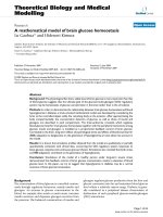
Figure 6 presents the results of computer simulation of

movement kinematics of UAV as well as the head axis during


8

Journal of Applied Mathematics
20
1500

10
UAV flight path

500
0
1000

Target interception
Scan lines
500
y(
m)

0
−500 −500

𝜗hr , 𝜓hr

−30
−40
−5

0

5

10

15
20
𝜗h , 𝜗hr (deg)

25

30

35

Figure 9: Real and desired trajectory of movement of the head axis
for nonoptimum controls with the influence of disturbances.

400
Path of target

300

0.8

200

0.6

100

Mex

0.4
0

Target interception

Min , Mex (Nm)

y (m)

−10
−20

Path of the target
1000
500
0
)
x (m

Figure 6: Path of movement of UAV, head axis, and the target during
searching for and tracking the target.

−100
−200
Path of head

−300
−400

−200

0

200
400
x (m)

600

800

1000

0
−0.2

Min

−0.4

−0.8

0

5

10

15
t (s)

20

25

30

Figure 10: Time-dependent control moments 𝑀in and 𝑀ex for
nonoptimum parameters of the regulator with the influence of
disturbances.

40
𝜓hr
30
20

𝜓h

10
0
−10
𝜗hr
−20
𝜗h
−30
−40

0.2

−0.6

Figure 7: Path of movement of point 𝐻 and the target on the surface
of the ground.

𝜓h , 𝜓hr , 𝜗h , 𝜗hr (deg)

𝜗h , 𝜓 h

0
𝜓h , 𝜓hr (deg)

z (m)

1000

0

5

10

15

20

25

30

t (s)

Figure 8: Time-dependent real 𝜗ℎ , 𝜓ℎ and desired 𝜗ℎ𝑟 , 𝜓ℎ𝑟 angles
specifying the location of the head axis for nonoptimum controls
with the influence of disturbances.

searching the surface of the ground and tracking (laser
lighting) a ground target.
Figure 7 presents the trajectory of movement of point 𝐻
during scanning for and the movement of the target on the
surface of the ground.
Figures 8–10 present the desired and the real angles
of deflection and inclination of the head axis, as well as
control moments for the case when the head is influenced by
kinematic excitations from UAV deck and the parameters of
the regulator are not optimum.
Figures 11, 12, and 13 present the desired and the real
angles of deflection and inclination of the head axis, as well as
control moments for the case when the head is not influenced
by kinematic excitations from UAV deck and the parameters
of the regulator are optimum.


Journal of Applied Mathematics

9

40

0.4
𝜓hr

30

0.3

𝜗h

0.2

10
0

𝜓h

−10

0
−0.1
−0.2

−20

Min

−0.3

−30
−40

Mex

0.1

Min , Mex (Nm)

𝜓h , 𝜓hr , 𝜗h , 𝜗hr (deg)

20

𝜗hr
0

5

10

15

20

−0.4
25

−0.5

30

0

5

10

t (s)

15

20

25

30

t (s)

Figure 11: Time-dependent real 𝜗ℎ , 𝜓ℎ and desired 𝜗ℎ𝑟 , 𝜓ℎ𝑟 angles
specifying the location of the head axis for optimum controls
without the influence of disturbances.

Figure 13: Time-dependent control moments 𝑀in and 𝑀ex for
optimum parameters of the regulator without the influence of
disturbances.
40

𝜓hr

20
30
𝜗h

𝜗h , 𝜓h

0
𝜓h , 𝜓hr (deg)

𝜓h

20
𝜓h , 𝜓hr , 𝜗h , 𝜗hr (deg)

10

−10
−20

10
0
−10
−20

𝜗hr , 𝜓hr

−40
−40
−5

𝜗hr

−30

−30

0

5

10
15
20
𝜗h , 𝜗hr (deg)

25

30

35

Figure 12: Real and desired trajectory of movement of the head axis
for optimum controls without the influence of disturbances.

Figures 14–16 present the desired and the real angles
of deflection and inclination of the head axis, as well as
control moments for the case when the head is influenced by
kinematic excitations from UAV deck and the parameters of
the regulator are optimum.
Kinematic excitations from UAV deck adversely affect the

operation of the head. It can particularly be seen in Figures 11
and 14. In case of the nonoptimum choice of the parameters
of the regulator, the deviations of the head axis from the set
location are particularly visible (Figures 8 and 9). Smaller
values of deviations can of course be achieved for optimum
head controls (Figures 14 and 15). Control moments take
small values.
From the presented theoretical analysis and the simulation research of the process of scanning by OTH from UAV

0

5

10

15
t (s)

20

25

30

Figure 14: Time-dependent real 𝜗ℎ , 𝜓ℎ and desired 𝜗ℎ𝑟 , 𝜓ℎ𝑟 angles
specifying the location of the head axis for optimum controls with
the influence of disturbances.

deck of the surface of the ground and then tracking the
detected ground target, it can be inferred that

(i) it is possible to search for a target on the area of any
size, which is only limited to the durability and range
of UAV flight;
(ii) scanning is sufficiently precise;
(iii) the programme of scanning the surface of the ground
is simple;
(iv) there occur relatively small values of OTH axis angle
deviations from the nominal position;
(v) full autonomy of UAV during the mission of searching
and laser lighting of the detected ground target
secures the point of control against detection and
destruction by an enemy;


10

Journal of Applied Mathematics
moment of passing from scanning to tracking mode were
minimized and disappeared in the shortest possible time.

20
10

Conflict of Interests
𝜓h , 𝜓hr (deg)

0

𝜗h , 𝜓 h

The authors declare that there is no conflict of interests
regarding the publication of this paper.

−10
−20

Acknowledgment

𝜗hr , 𝜓hr

The work reported herein was undertaken as part of a
research project supported by the National Centre for
Research and Development over the period 2011–2014.

−30
−40
−5

0

5

10

15

20

25

30

35

𝜗h , 𝜗hr (deg)

Figure 15: Real and desired trajectory of movement of the head axis
for optimum controls with the influence of disturbances.
0.8
Mex

0.6

Min , Mex (Nm)

0.4
0.2
0
−0.2
−0.4

Min

−0.6
−0.8

0

5

10

15
t (s)

20

25

30

Figure 16: Time-dependent control moments 𝑀in and 𝑀ex for
optimum parameters of the regulator without the influence of
disturbances.

(vi) the interference of an operator in controlling UAV
may only be limited to cases of the vehicle’s total coming off from the set path or the loss of the target from
OTH lens coverage (due to gusts of wind, explosions
of missiles, etc.). Hence, the possibility of automatic
sending of information about such occurrences to the
control point and the possible taking of control over
UAV flight by the operator should be introduced.

5. Conclusion
The considerations presented in this paper will allow us
to conduct the research on the dynamics of OTH when
manoeuvring UAV on which this device is mounted. It may
enable the construction engineers to choose such parameters
of OTH so that the transient processes occurring in the
conditions of kinematic influence of UAV deck and at the

References
[1] R. Austin, Unmanned Aircraft Systems: UAVS Design, Development and Deployment, John Wiley & Sons, Chichester, UK,
2010.
[2] F. Kamrani and R. Ayani, UAV Path Planning in Search Operations, Aerial Vehicles, InTech, 2009, edited by T. M. Lam.
[3] X. Q. Chen, Q. Ou, D. R. Wong et al., “Flight dynamics
modelling and experimental validation for unmanned aerial
vehicles,” in Mobile Robots-State of the Art in Land, Sea, Air, and
Collaborative Missions, X. Q. Chen, Ed., InTech, 2009.
[4] S. Bhandari, R. Colgren, P. Lederbogen, and S. Kowalchuk,
“Six-DoF dynamic modeling and flight testing of a UAV
helicopter,” in Proceedings of the AIAA Modeling and Simulation
Technologies Conference, pp. 992–1008, San Francisco, Calif,
USA, August 2005.
[5] J. Manerowski and D. Rykaczewski, “Modelling of UAV flight
dynamics using perceptron artificial neural networks,” Journal
of Theoretical and Applied Mechanics, vol. 43, no. 2, pp. 297307,
2005.
ă
[6] K. T. Oner,
E. C
á etinsoy, E. Sirimoˇglu et al., “Mathematical
modeling and vertical flight control of a tilt-wing UAV,” Turkish
Journal of Electrical Engineering and Computer Sciences, vol. 20,
no. 1, pp. 149–157, 2012.
[7] T.-V. Chelaru, V. Pana, and A. Chelaru, “Flight dynamics for
UAV formations,” in Proceedings of the 10th WSEAS International Conference on Automation & Information, pp. 287–292,
2009.
[8] P. Kanovsky, L. Smrcek, and C. Goodchild, “Simulation of UAV
Systems,” Acta Polytechnica, vol. 45, no. 4, pp. 109–113, 2005.

[9] H. Ergezer and K. Leblebicioglu, “Planning unmanned aerial
vehicles path for maximum information collection using evolutionary algorithms,” in Proceedings of the 18th IFAC World
Congress, pp. 5591–5596, Milano, Italy, 2011.
[10] C. Sabo and K. Cohen, “Fuzzy logic unmanned air vehicle
motion planning,” Advances in Fuzzy Systems, vol. 2012, Article
ID 989051, 14 pages, 2012.
[11] H. Chen, K. Chang, and C. S. Agate, “Tracking with UAV using
tangent-plus-lyapunov vector field guidance,” in Proceedings
of the 12th International Conference on Information Fusion
(FUSION '09), pp. 363–372, Seattle, Wash, USA, July 2009.
[12] K. Turkoglu, U. Ozdemir, M. Nikbay et al., “PID parameter
optimization of an UAV longitudinal flight control system,” Proceedings of World Academy of Science: Engineering & Technology,
vol. 2, no. 9, pp. 24–29, 2008.


Journal of Applied Mathematics
[13] B. Kada and Y. Ghazzawi, “Robust PID controller design for an
UAV flight control system,” in Proceedings of the World Congress
on Engineering and Computer Science (WCECS ’11), vol. 2, San
Francisco, Calif, USA, October 2011.
[14] I. Moir and A. Seabridge, Military Avionics Systems, John Wiley
& Sons, Chichester, UK, 2007.
[15] J. Awrejcewicz and Z. Koruba, Classical Mechanics: Applied
Mechanics and Mechatronics, vol. 30, Springer, New York, NY,
USA, 2012.
[16] I. Krzysztofik, “The dynamics of the controlled observation
and tracking head located on a moving vehicle,” Solid State
Phenomena, vol. 180, pp. 313–322, 2012.
[17] Z. Koruba, “Optimal control of the searching and tracking
head (Sth) for self propelled anti aircraft vehicle,” Solid State

Phenomena, vol. 180, pp. 27–38, 2012.
[18] R. Langton, Stability and Control of Aircraft Systems, John Wiley
& Sons, Chichester, UK, 2007.
[19] J. E. Takosoglu, P. A. Laski, and S. Blasiak, “A fuzzy logic
controller for the positioning control of an electro-pneumatic
servo-drive,” Proceedings of the Institution of Mechanical Engineers I: Journal of Systems and Control Engineering, vol. 226, no.
10, pp. 1335–1343, 2012.

11


Copyright of Journal of Applied Mathematics is the property of Hindawi Publishing
Corporation and its content may not be copied or emailed to multiple sites or posted to a
listserv without the copyright holder's express written permission. However, users may print,
download, or email articles for individual use.