Electronic Circuits - Part 2 - Chapter 11 Frequency Response pdf
Bạn đang xem bản rút gọn của tài liệu. Xem và tải ngay bản đầy đủ của tài liệu tại đây (2.3 MB, 25 trang )
[1] Behzad Razavi: Fundamentals of Microelectronics,
1st Edition, 2008.
[2] D.L. Schilling, Charles Belove : Electronic Circuits:
Discrete and Integrated , Mc Graw-Hill Inc, 1968, 1992,
[4] Robert Boylestad, Louis Nashelsky, Electronic Devices
and Circuit Theory, Prentice Hall, 2008.
[5] Lê Tiến Thường, Giáo trình mạch điện tử 2, ĐH Bách
Khoa Tp.HCM, 2009
Teacher: Dr. LUU THE VINH
Contents
TIMES
PAGE
11
FREQUENCY RESPONSE
9
537(544)
13
OUTPUT STAGES AND POWER
AMPLIFIERS
12
685 (694)
14
ANALOG FILTERS
6
721 (731)
15
DIGITAL CMOS CIRCUITS
6
775(786)
16
CMOS AMPLIFIERS
6
0 (829)
Appendix
Introduction to SPICE
6
817(909)
45
0
CHAPTER
CONTENTS
SUM
Frequency Response
FREQUENCY RESPONSE
The need for operating circuits at increasingly higher
speeds has always challenged designers. From radar and
television systems in the 1940s to gigahertz microprocessors
today, the demand for pushing circuits to higher frequencies
has required a solid understanding of their speed limitations.
In this chapter, we study the effects that limit the speed
of transistors and circuits, identifying topologies that better
lend themselves to high-frequency operation. We also
develop skills for deriving transfer functions of circuits, a
critical task in the study of stability and frequency
compensation (12). We assume bipolar transistors remain in
the active mode and MOSFETs in the saturation region.
1
11.1 Fundamental Concepts
What do we mean by “frequency response?”
• 11.1.1 General Considerations
What do we mean by “frequency response?” Illustrated
in Fig. 11.1(a), the idea is to apply a sinusoid at the input of
the circuit and observe the output while the input frequency
is varied. As exemplified by Fig. 11.1(a), the circuit may
exhibit a high gain at low frequencies but a “roll-off” as the
frequency increases. We plot the magnitude of the gain as
in Fig. 11.1(b) to represent the circuit’s behavior at all
frequencies of interest. We may loosely call f1 the useful
bandwidth of the circuit. Before investigating the cause of
this roll-off, we must ask: why is frequency response
important? The following examples illustrate the issue.
Figure 11.1 (a) Conceptual test of frequency response, (b) gain roll-off with
frequency.
Vd: Đáp ứng tần số của một mạch KĐ – Miền thời gian
Vd: Đáp ứng tần số của một mạch KĐ – Miền thời gian
8.0mA
8.0mA
Ic (mA)
Ic (mA)
4.0mA
4.0mA
0A
0A
-4.0mA
0s
5s
I(Iin)
IC(Q1)
Time
Tần số = 1Hz
Vd: Đáp ứng tần số của một mạch KĐ – Miền thời gian
8.0mA
10s
t (s)
-4.0mA
0s
50ms
I(Iin)
IC(Q1)
Time
100ms
t (s)
Tần số = 100Hz
Vd: Đáp ứng tần số của một mạch kđ – Miền tần số
8.0mA
Ic (mA)
Ic (mA)
4.0mA
4.0mA
0A
0A
-4.0mA
0s
I(Iin)
0.5ms
IC(Q1)
Time
Tần số = 10KHz
1.0ms
t (s)
-4.0mA
0s
5us
I(Iin)
IC(Q1)
Time
10us
t (s)
Tần số = 1MHz
2
Vd: Đáp ứng tần số của một mạch kđ – Miền tần số
Vd: Đáp ứng tần số của một mạch kđ – Miền tần số
200
120
A
A(dB)
80
100
40
0
1.0Hz
10Hz
I(RC)/ I(Iin)
100Hz
1.0KHz
10KHz
Frequency
100KHz
1.0MHz
10MHz
F (Hz)
0
1.0Hz
10Hz
100Hz
20*LOG(I(RC)/I(Iin))
Explain why people’s voice over the phone sounds different from their voice in
face-to-face conversation.
Solution.
• Human voice contains frequency components from 20 Hz to 20 kHz
[Fig. 11.2(a)]. Thus, circuits processing the voice must accommodate
this frequency range. Unfortunately, the phone system suffers from a
limited bandwidth, exhibiting the frequency response shown in Fig.
11.2(b). Since the phone suppresses frequencies above 3.5 kHz,
each person’s voice is altered. In high-quality audio systems, on the
other hand, the circuits are designed to cover the entire frequency
range.
10KHz
100KHz
Frequency
Gain = Iout / Iin
Example 11.1
1.0KHz
1.0MHz
10MHz
F (Hz)
GaindB = 20*log(Iout / Iin)
Frequency Response
• Exercise.
Whose voice does the phone system alter more,
men’s or women’s?
• Giọng nói nào bị thay đổi nhiều hơn khi nghe qua
điện thoại, nam giới hay phụ nữ?
Example 11.2
When you record your voice and listen to it, it sounds some what
different from the way you hear it directly when you speak. Explain
why?
Solution
During recording, your voice propagates through
the air and reaches the audio recorder. On the other
hand, when you speak and listen to your own voice
simultaneously, your voice propagates not only
through the air but also from your mouth through
your skull to your ear. Since the frequency response
of the path through your skull is different from that
through the air (i.e., your skull passes some
frequencies more easily than others), the way you
hear your own voice is
different from the way other people hear your voice.
•• Exercise
Exercise
Giải thích những gì sẽ xảy ra với giọng nói
Giải thích những gì sẽ xảy ra với giọng nói
của bạn khi bạn bị cảm lạnh?
của bạn khi bạn bị cảm lạnh?
3
Example 11.3
Video signals typically occupy a bandwidth of about 5 MHz. For
example, the graphics card delivering the video signal to the
display of a computer must provide at least 5 MHz of
bandwidth. Explain what happens if the bandwidth of a video
system is insufficient.
Frequency Response
The display is scanned from left to right
•Solution
With insufficient bandwidth, the “sharp” edges on a
display become “soft,” yielding a fuzzy picture. This is
because the circuit driving the display is not fast enough to
abruptly change the contrast from, e.g., complete white to
complete black from one pixel to the next.
Figures 11.3(a) and (b) illustrate this effect for a highbandwidth and low-bandwidth driver, respectively. (The display
is scanned from left to right.)
Frequency Response
• What causes the gain roll-off in Fig. 11.1? As a simple
example, let us consider the low-pass filter depicted in Fig.
11.4(a). At low frequencies, C1 is nearly open and the
current through R1 nearly zero; thus,Vout = Vin. As the
frequency increases, the impedance of C1 falls and the
voltage divider consisting of R1 and C1 attenuates Vin to a
greater extent. The circuit therefore exhibits the behavior
shown in Fig. 11.4(b).
Figure 11.4 (a) Simple low-pass filter, and (b) its frequency response.
Figure 11.3
• Exercise
What happens if the display is scanned from top
to bottom?
As a more interesting example, consider the
common-source stage illustrated in Fig. 11.5(a),
where a load capacitance,CL, appears at the output.
At low frequencies, the signal current produced by
M1 prefers to flow through RD because the
impedance of CL,1/(CLs), remains high. At high
frequencies, on the other hand, CL “steals” some of
the signal current and shunts it to ground, leading to
a lower voltage swing at the output. In fact, from the
small-signal equivalent circuit of Fig. 11.5(b), we
note that RD and CL are in parallel and hence:
1
Vout g mVin RD / /
CL s
(11.1)
11.1.2. Relationship Between Transfer Function and
11.1.2. Relationship Between Transfer Function and
Frequency Response
Frequency Response
• We know from basic circuit theory that the transfer
function of a circuit can be written as:
a)
(11.2)
b)
Figure 11.5 (a) CS stage with load capacitance,
(b) small-signal model of the circuit.
Where A0 denotes the low frequency gain because H(s)
A0 as s 0. The frequencies zj an pj represent the
zeros and poles of the transfer function, respectively.
4
•• If the input to the circuit is a sinusoid of the form
If the input to the circuit is a sinusoid of the form
x(t) = Acos(2ft) = Acost, then the output can be
x(t) = Acos(2ft) = Acost, then the output can be
expressed as
expressed as
Example 11.4
Example 11.4
Determine the transfer function and frequency response of the CS
Determine the transfer function and frequency response of the CS
stage shown in Fig. 11.5(a).
stage shown in Fig. 11.5(a).
(11.3)
Where H(j) is obtained by making the substitution s = j.
Where H(j) is obtained by making the substitution s = j.
Called the “magnitude” and the “phase,” /H(j)/ and
Called the “magnitude” and the “phase,” /H(j)/ and
H(j) respectively reveal the frequency response of the
H(j) respectively reveal the frequency response of the
circuit. In this chapter, we are primarily concerned with the
circuit. In this chapter, we are primarily concerned with the
former. Note that ff (in Hz) and (in radians per second) are
former. Note that (in Hz) and (in radians per second) are
related by a factor of 2.
related by a factor of 2.
For example, we may write = 5.1010 rad/s =2(7,96 GHz).
For example, we may write = 5.1010 rad/s =2(7,96 GHz).
Solution
Solution
Fig. 11.5(a).
As expected, the gain begins at gmRD at low frequencies,
rolling off as
becomes comparable with unity. At
=1/RDCL:
From Eq. (11.1), we have:
(11.7)
(11.4)
(11.5)
Since 20 log 2 3 dB, we say the -3-dB bandwidth of
Since 20 log 2 3 dB, we say the -3-dB bandwidth of
the circuit is equal to 1/(RDCL))(Fig.11.6).
the circuit is equal to 1/(RDCL (Fig.11.6).
For a sinusoidal input, we replace s = j and compute the
magnitude of the transfer function:
(11.6)
Exercise
Exercise
Derive the above results if 0.
Derive the above results if 0.
• Example 11.5.
Consider the common-emitter stage shown in Fig.
11.7. Derive a relationship between the gain the 3-dB
bandwidth, and the power consumption of the circuit.
Figure 11.6
Exercise
Exercise
Derive the above results if 0.
Derive the above results if 0.
••Example 11.5.
Example 11.5.
Xét mạch KĐ CE trên hình. 11,7. xác định mối quan hệ giữa
Xét mạch KĐ CE trên hình. 11,7. xác định mối quan hệ giữa
độ lợi băng thông 3 dB, và công suất tiêu thụ năng lượng của
độ lợi băng thông 3 dB, và công suất tiêu thụ năng lượng của
mạch..
mạch
5
Solution
Solution
In a manner similar to the CS topology of Fig. 11.5(a),
In a manner similar to the CS topology of Fig. 11.5(a),
the bandwidth is given by 1=/(RCCLL),
the bandwidth is given by 1=/(RCC ),
the low-frequency gain by gmRC =(IC/VTT )RC, and the
the low-frequency gain by gmRC =(IC/V )RC, and the
power consumption by IC .VCC..For the highest
power consumption by IC .VCC For the highest
performance, we wish to maximize both the gain and the
performance, we wish to maximize both the gain and the
bandwidth (and hence the product of the two) and
bandwidth (and hence the product of the two) and
minimize the power dissipation. We therefore define a
minimize the power dissipation. We therefore define a
“figure of merit” as:
“figure of merit” as:
Solution
Solution
In a manner similar to the CS topology of Fig. 11.5(a),
In a manner similar to the CS topology of Fig. 11.5(a),
the bandwidth is given by 1=/(RCCLL), the low-frequency
the bandwidth is given by 1=/(RCC ), the low-frequency
gain by gmRC =(IC/VTT )RC, and the power consumption by
gain by gmRC =(IC/V )RC, and the power consumption by
IIC .VCC..
C .VCC
Để hiệu suất cao nhất, ta phải tối đa hóa cả độ lợi và
Để hiệu suất cao nhất, ta phải tối đa hóa cả độ lợi và
băng thơng (và do đó sản phẩm của hai) và giảm thiểu
băng thông (và do đó sản phẩm của hai) và giảm thiểu
cơng suất tiêu tán. Do đó:
cơng suất tiêu tán. Do đó:
(11.8)
(11.8)
(11.9)
(11.9)
Example 11.6
Example 11.6
Explain the relationship between the frequency response and
Explain the relationship between the frequency response and
step response of the simple lowpass filter shown in Fig. 11.4(a).
step response of the simple lowpass filter shown in Fig. 11.4(a).
Solution
To obtain the transfer function, we view the circuit
as a voltage divider and write
(11.10)
a)
(11.11)
b)
Fig. 11.4
•• The frequency response is determined by
The frequency response is determined by
replacing s with j and computing the magnitude:
replacing s with j and computing the magnitude:
(11.2)
The 3-dB bandwidth is equal to 1/(R11C1). The circuit’s
The 3-dB bandwidth is equal to 1/(R C1). The circuit’s
response to a step of the form Vout(t) is given by
response to a step of the form Vout(t) is given by
(11.3)
•• The relationship between (11.12) and (11.13) is
The relationship between (11.12) and (11.13) is
that, as R11C1 increases, the bandwidth drops
that, as R C1 increases, the bandwidth drops
and the step response becomes slower. Figure
and the step response becomes slower. Figure
11.8 plots this behavior, revealing that a narrow
11.8 plots this behavior, revealing that a narrow
bandwidth results in a sluggish time response. This
bandwidth results in a sluggish time response. This
observation explains the effect seen in Fig. 1.3(b):
observation explains the effect seen in Fig. 1.3(b):
since the signal cannot rapidly jump from low
since the signal cannot rapidly jump from low
(white) to high (black), it spends some time at
(white) to high (black), it spends some time at
intermediate levels (shades of gray), creating
intermediate levels (shades of gray), creating
“fuzzy” edges.
“fuzzy” edges.
6
Exercise
Exercise
At what frequency does /H/ fall by a factor of two?
At what frequency does /H/ fall by a factor of two?
11.1.3 Bode’s Rules
11.1.3 Bode’s Rules
•• The task of obtaining /H(j)/ from H(s) and plotting the result is some
The task of obtaining /H(j)/ from H(s) and plotting the result is some
what tedious. For this reason, we often utilize Bode’s rules
what tedious. For this reason, we often utilize Bode’s rules
(approximations) to construct /H(j)/ rapidly. Bode’s rules for /H(j)/
(approximations) to construct /H(j)/ rapidly. Bode’s rules for /H(j)/
are as follows:
are as follows:
•• As passes each pole frequency, the slope of /H(j)/
As passes each pole frequency, the slope of /H(j)/
Figure 11.8
•• Example 11.7
Example 11.7
•• Construct the Bode plot of |H(j)| for the CS stage
Construct the Bode plot of |H(j)| for the CS stage
depicted in Fig. 11.5(a).
depicted in Fig. 11.5(a).
decreases by 20 dB/dec; (A slope of 20 dB/dec simply
decreases by 20 dB/dec; (A slope of 20 dB/dec simply
means a tenfold change in for a tenfold increase in
means a tenfold change in for a tenfold increase in
frequency.)
frequency.)
•• As passes each zero frequency, the slope of j
As passes each zero frequency, the slope of j
increases by 20 dB/dec.
increases by 20 dB/dec.
Solution
Solution
Equation (11.5) indicates a pole frequency of
Equation (11.5) indicates a pole frequency of
p1
1
RD CL
(11.14),
The magnitude thus begins at gmRD at low frequencies and
The magnitude thus begins at gmRD at low frequencies and
remains flat up to = |p1 |.At this point, the slope changes
remains flat up to = |p1 |.At this point, the slope changes
from zero to 20 dB/dec. Figure 11.9 illustrates the result. In
from zero to 20 dB/dec. Figure 11.9 illustrates the result. In
contrast to Fig. 11.5(b), the Bode approximation ignores the
contrast to Fig. 11.5(b), the Bode approximation ignores the
3-dB roll-off at the pole frequency but it greatly simplifies the
3-dB roll-off at the pole frequency but it greatly simplifies the
algebra. As evident from Eq. (11.6), for R22D C22L22>> 1,
algebra. As evident from Eq. (11.6), for R D C L >> 1,
Bode’s rule provides a good approximation.
Bode’s rule provides a good approximation.
Exercise
• Construct the Bode plot for g =(150)-1; RD
=2k, and CL =100 fF.
Figure 11.9
7
11.1.4 Association of Poles with Nodes
•• The poles of a circuit’s transfer function play a central role
The poles of a circuit’s transfer function play a central role
in the frequency response. The designer must therefore be
in the frequency response. The designer must therefore be
able to identify the poles intuitively so as to determine
able to identify the poles intuitively so as to determine
which parts of the circuit appear as the “speed bottleneck.”
which parts of the circuit appear as the “speed bottleneck.”
•• The CS topology studied in Example 11.4 serves as a
The CS topology studied in Example 11.4 serves as a
good example for identifying poles by inspection. Equation
good example for identifying poles by inspection. Equation
(11.5) reveals that the pole frequency is given by the
(11.5) reveals that the pole frequency is given by the
inverse of the product of the total resistance seen between
inverse of the product of the total resistance seen between
the output node and ground and the total capacitance seen
the output node and ground and the total capacitance seen
between the output node and ground. Applicable to many
between the output node and ground. Applicable to many
circuits, this observation can be generalized as follows: if
circuits, this observation can be generalized as follows: if
node jjin the signal path exhibits a small-signal resistance
node in the signal path exhibits a small-signal resistance
of Rj to ground and a capacitance of Cj to ground, then it
of Rj to ground and a capacitance of Cj to ground, then it
contributes a pole of magnitude (RjCj) -1 to the transfer
contributes a pole of magnitude (RjCj) -1 to the transfer
function.
function.
Solution
• Setting Vin to zero, we recognize that the gate of
M1 sees a resistance of RS and a capacitance of
Cin to ground. Thus,
Example 11.8. Determine the poles of the circuit shown in
Example 11.8. Determine the poles of the circuit shown in
Fig. 11.10. Assume =0 (: channel – length modulation
Fig. 11.10. Assume =0 (: channel – length modulation
coeffient)
coeffient)
Figure 11.10 .
•• Since the low-frequency gain of the circuit is
Since the low-frequency gain of the circuit is
equal to -- gmRD,, we can readily write the
equal to gmRD we can readily write the
magnitude of the transfer function as:
magnitude of the transfer function as:
(11.17)
(11.15)
We may call p1 the “input pole” to indicate that it
arises in the input network. Similarly, the “output
pole” is given by
(11.16)
Example 11.9
Example 11.9
•• Compute the poles of the circuit shown in Fig.
Compute the poles of the circuit shown in Fig.
11.11. Assume =0.
11.11. Assume =0.
Exercise.
If p1= p2’ at what frequency does the gain
drop by 3 dB?
Solution
Solution
•• With Vin = 0, the small-signal resistance seen at the
With Vin = 0, the small-signal resistance seen at the
source of M1 is given by RS//(1/gm), yielding a pole at
source of M1 is given by RS//(1/gm), yielding a pole at
(11.18)
The output pole is given by ..
The output pole is given by
P2 = (RDCL)-1
8
11.1.5 Miller’s Theorem
11.1.5 Miller’s Theorem
11.1.5 Miller’s Theorem
11.1.5 Miller’s Theorem
Figure 11.13
Figure 11.13
(a) General circuit including a floating impedance,
(a) General circuit including a floating impedance,
(b) equivalent of (a) as obtained from Miller’s theorem.
(b) equivalent of (a) as obtained from Miller’s theorem.
Thus,
(11.19)
•• Consider the general circuit shown in Fig. 11.13(a), where
Consider the general circuit shown in Fig. 11.13(a), where
the floating impedance, ZFF,appears between nodes 1 and
the floating impedance, Z ,appears between nodes 1 and
2. We wish to transform ZFFto two grounded impedances as
2. We wish to transform Z to two grounded impedances as
depicted in Fig. 11.13(b), while ensuring all of the currents
depicted in Fig. 11.13(b), while ensuring all of the currents
and voltages in the circuit remain unchanged.
and voltages in the circuit remain unchanged.
•• To determine Z1 and Z2, we make two observations: (1)
To determine Z1 and Z2, we make two observations: (1)
the current drawn by ZFFfrom node 1 in Fig. 11.13(a) must
the current drawn by Z from node 1 in Fig. 11.13(a) must
be equal to that drawn by Z1 in Fig. 11.13(b); and (2) the
be equal to that drawn by Z1 in Fig. 11.13(b); and (2) the
current injected to node 2 in Fig. 11.13(a)must be equal to
current injected to node 2 in Fig. 11.13(a)must be equal to
that injected by Z22in Fig. 11.13(b). (These requirements
that injected by Z in Fig. 11.13(b). (These requirements
guarantee that the circuit does not “feel” the
guarantee that the circuit does not “feel” the
transformation.)
transformation.)
and
(11.23)
(11.20)
(11.24)
Denoting the voltage gain from node 1 to node 2 by Av ,
v
we obtain
(11.21)
(11.22)
Called Miller’s theorem, the results expressed by
Called Miller’s theorem, the results expressed by
(11.22) and (11.24) prove extremely useful in
(11.22) and (11.24) prove extremely useful in
analysis and design. In particular, (11.22) suggests
analysis and design. In particular, (11.22) suggests
that the floating impedance is reduced by a factor of
that the floating impedance is reduced by a factor of
1 -- Av when “seen” at node 1.
1 Av when “seen” at node 1.
Ex. Let us assume ZF is a single capacitor, CF ,, tied
Ex. Let us assume ZF is a single capacitor, CF tied
between the input and output of an inverting
between the input and output of an inverting
amplifier [Fig. 11.14(a)]. Applying (11.22),we have
amplifier [Fig. 11.14(a)]. Applying (11.22),we have
(11.25)
(11.26)
Figure 11.14 (a) Inverting circuit with floating capacitor,
Figure 11.14 (a) Inverting circuit with floating capacitor,
(b) equivalent circuit as obtained from Miller’s theorem.
(b) equivalent circuit as obtained from Miller’s theorem.
9
•• where the substitution Av = -A00 is made. What
where the substitution Av = -A is made. What
type of impedance is Z1?
type of impedance is Z1?
•• The 1/s dependence suggests a capacitor of
The 1/s dependence suggests a capacitor of
value (1+A00)CF, as if CF is “amplified” by a factor
value (1+A )CF, as if CF is “amplified” by a factor
of 1+A00. In other words, a capacitor CF tied
of 1+A . In other words, a capacitor CF tied
between the input and output of an inverting
between the input and output of an inverting
amplifier with a gain of A00 raises the input
amplifier with a gain of A raises the input
capacitance by an amount equal to (1+A00)CF ..
capacitance by an amount equal to (1+A )CF
We say such a circuit suffers from “Miller
We say such a circuit suffers from “Miller
multiplication” of the capacitor.
multiplication” of the capacitor.
•• The Miller multiplication of capacitors can also be
The Miller multiplication of capacitors can also be
explained intuitively. Suppose the input voltage in
explained intuitively. Suppose the input voltage in
Fig. 11.14(a) goes up by a small amount V ..
Fig. 11.14(a) goes up by a small amount V
The output then goes down by A00V ..
The output then goes down by A V
•• That is, the voltage across CF increases by (1 +
That is, the voltage across CF increases by (1 +
A00)V ,, requiring that the input provide a
A )V requiring that the input provide a
proportional charge. By contrast, if CF were not a
proportional charge. By contrast, if CF were not a
floating capacitor and its right plate voltage did
floating capacitor and its right plate voltage did
not change, it would experience only a voltage
not change, it would experience only a voltage
change of V and require less charge.
change of V and require less charge.
•• The above study points to the utility of Miller’s
The above study points to the utility of Miller’s
theorem for conversion of floating capacitors to
theorem for conversion of floating capacitors to
grounded capacitors. The following example
grounded capacitors. The following example
demonstrates this principle.
demonstrates this principle.
The effect of CFFat the output can be obtained from (11.24):
The effect of C at the output can be obtained from (11.24):
(11.27)
(11.28)
-1
which is close to (CFs))-1if A0 >>1 .. Figure 11.14(b)
which is close to (CFs if A0 >>1 Figure 11.14(b)
summarizes these results.
summarizes these results.
Example 11.10
Example 11.10
•• Estimate the poles of the circuit shown in Fig.
Estimate the poles of the circuit shown in Fig.
11.15(a). Assume =0.
11.15(a). Assume =0.
Figure 11.15
Figure 11.15
Solution
Solution
Noting that M1 and RD constitute an inverting
Noting that M1 and RD constitute an inverting
amplifier having a gain of –gmRD,, we utilize the
amplifier having a gain of –gmRD we utilize the
results in Fig. 11.14(b) to write:
results in Fig. 11.14(b) to write:
(11.29)
(11.32)
(11.33)
and
(11.30)
(11.34)
and
(11.31)
Thereby arriving at the topology depicted in Fig.
Thereby arriving at the topology depicted in Fig.
11.15(b). From our study in Example 11.8, we have:
11.15(b). From our study in Example 11.8, we have:
(11.35)
10
The reader may find the above example some what
The reader may find the above example some what
inconsistent. Miller’s theorem requires that the floating
inconsistent. Miller’s theorem requires that the floating
impedance and the voltage gain be computed at the same
impedance and the voltage gain be computed at the same
frequency where as Example 11.10 uses the low-frequency
frequency where as Example 11.10 uses the low-frequency
gain. gmRD,,even for the purpose of finding high-frequency
gain. gmRD even for the purpose of finding high-frequency
poles. After all, we know that the existence of CFFlowers the
poles. After all, we know that the existence of C lowers the
voltage gain from the gate of M1 to the output at high
voltage gain from the gate of M1 to the output at high
frequencies. Owing to this inconsistency, we call the
frequencies. Owing to this inconsistency, we call the
procedure in Example 11.10 the “Miller approximation.”
procedure in Example 11.10 the “Miller approximation.”
Without this approximation, i.e., if A0 is expressed in
Without this approximation, i.e., if A0 is expressed in
of circuit parameters at the frequency of interest, application of
of circuit parameters at the frequency of interest, application of
Miller’s theorem would be no simpler than direct solution of
Miller’s theorem would be no simpler than direct solution of
the circuit’s equations.
the circuit’s equations.
Another artifact of Miller’s approximation is that
Another artifact of Miller’s approximation is that
it may eliminate a zero of the transfer function. We
it may eliminate a zero of the transfer function. We
return to this issue in Section 11.4.3.
return to this issue in Section 11.4.3.
The general expression in Eq. (11.22) can be
The general expression in Eq. (11.22) can be
interpreted as follows: an impedance tied between
interpreted as follows: an impedance tied between
the input and output of an inverting amplifier with a
the input and output of an inverting amplifier with a
gain of Av is lowered by a factor of 1+ Av if seen at
gain of Av is lowered by a factor of 1+ Av if seen at
the input (with respect to ground). This reduction of
the input (with respect to ground). This reduction of
impedance (hence increase in capacitance) is called
impedance (hence increase in capacitance) is called
“Miller effect.” For example, we say Miller effect
“Miller effect.” For example, we say Miller effect
raises the input capacitance of the circuit in Fig.
raises the input capacitance of the circuit in Fig.
11.15(a) to (1 + gmRD)CF ..
11.15(a) to (1 + gmRD)CF
11.1.6 General Frequency Response
Our foregoing study indicates that capacitances in a circuit tend to lower
Our foregoing study indicates that capacitances in a circuit tend to lower
the voltage gain at high frequencies. It is possible that capacitors reduce
the voltage gain at high frequencies. It is possible that capacitors reduce
the gain at low frequencies as well. As a simple example, consider the
the gain at low frequencies as well. As a simple example, consider the
high-pass filter shown in Fig. 11.16(a), where the voltage division
high-pass filter shown in Fig. 11.16(a), where the voltage division
between C and R yields
between C and R yields
and hence
Figure 11.16 (a) Simple high-pass filter, and (b) its frequency response.
Figure 11.16 (a) Simple high-pass filter, and (b) its frequency response.
Example 11.11
Example 11.11
• Figure 11.17 depicts a source follower used in a high-quality audio
amplifier. Here, establishes a gate bias voltage equal to VDD for M1,
and I 1 defines the drain bias current. Assume =0; gm=1/(200), and
R1 =100 k. Determine the minimum required value of C1 and the
maximum tolerable value of .
Figure 11.17
•• Plotted in Fig. 11.16(b), the response exhibits a roll-off as the
Plotted in Fig. 11.16(b), the response exhibits a roll-off as the
frequency of operation falls below 1/(R1C1). As seen from Eq. (11.37),
frequency of operation falls below 1/(R1C ). As seen from Eq. (11.37),
this roll-off arises because the zero of the 1 transferfunction occurs at
this roll-off arises because the zero of thetransfer function occurs at
the origin.
the origin.
•• The low-frequency roll-off may prove undesirable. The following
The low-frequency roll-off may prove undesirable. The following
example illustrates this point.
example illustrates this point.
Solution
• Similar to the high-pass filter of Fig. 11.16, the input
network consisting of Ri andCi attenuates the signal at
low frequencies. To ensure that audio components as low
as 20 Hz experience a small attenuation, we set the
corner frequency 1/RiCi to 2 x (20Hz) , thus obtaining
(11.39)
Ci = 79,6nF
This value is, of course, much to large to be
integrated on a chip. Since Eq. (11.38) reveals a
3dB attenuation at =1/(RiCi), in practice we
must choose even a larger capacitor if a lower
attenuation is desired.
11
• The load capacitance creates a pole at the output node,
lowering the gain at high frequencies. Setting the pole
frequency to the upper end of the audio range, 20 kHz,
and recognizing that the resistance seen from the output
node to ground is equal to 1/gm, we have
(11.40)
(11.41)
and hence
(11.42)
An efficient driver, the source follower can
tolerate a very large load capacitance (for the
audio band).
Exercise
Exercise
Repeat the above example if I1 and the width of M1 are halved.
Repeat the above example if I1 and the width of M1 are halved.
Why did we use capacitor Ci in the above example?
Without Ci, the circuit’s gain would not fall at low frequencies,
and we would not need perform the above calculations. Called
a “coupling” capacitor, Ci allows the signal frequencies of
interest to pass through the circuit while blocking the dc
content of Vin. Inother words, Ci isolates the bias conditions of
the source follower from those of the preceding stage. Figure
11.18(a) illustrates an example, where a CS stage precedes
the source follower. The coupling capacitor permits
independent bias voltages at nodes X and Y. For example, VY
can be chosen relatively low (placing M2 near the triode
region) to allow a large drop across RD, thereby maximizing
the voltage gain of the CS stage (why?).
To convince the reader that capacitive coupling proves
essential in Fig. 11.18(a), we consider the case of “direct
coupling” [Fig. 11.18(b)] as well. Here, to maximize the
voltage gain, we wish to set VP just above VGS2 - VTH2, e.g.,
200 mV. On the other hand, the gate of M2 must reside at a
voltage of at least VGS1 + VI1, where VI1 denotes the minimum
voltage required by I1. SinceVGS1 + VI1 may reach 600-700
mV, the two stages are quite incompatible in terms of their
bias points, necessitating capacitive coupling.
Figure 11.18. Cascade of CS stage and source follower
with (a) capacitor coupling and (b) direct coupling.
Cascade của CS giai đoạn và theo dõi nguồn với khớp nối tụ (a) và
(b) nối trực tiếp.
Capacitive coupling (also called “ac coupling”) is more common
in discrete circuit design due to the large capacitor values required in
many applications (e.g.,Ci in the above audio example). Nonetheless,
many integrated circuits also employ capacitive coupling, especially at
low supply voltages, if the necessary capacitor values are no more than
a few picofarads.
Figure 11.19 shows a typical frequency response and the
terminology used to refer to its various attributes. We call L the lower
corner or lower “cut-off” frequency and H the upper corner or upper cutoff frequency. Chosen to accommodate the signal frequencies of
interest, the band between L and H is called the “midband range” and
the corresponding gain the “midband gain.”
Figure 11.19. Typical frequency response.
12
11.2 High-Frequency Models of Transistors
11.2 High-Frequency Models of Transistors
The speed of many circuits is limited by the
The speed of many circuits is limited by the
capacitances within each transistor. It is therefore necessary to
capacitances within each transistor. It is therefore necessary to
study these capacitances carefully.
study these capacitances carefully.
11.2.1 High-Frequency Model of Bipolar Transistor
11.2.1 High-Frequency Model of Bipolar Transistor
Recall from Chapter 4 that the bipolar transistor consists
Recall from Chapter 4 that the bipolar transistor consists
of two PN junctions. The depletion region associated with the
of two PN junctions. The depletion region associated with the
junctions gives rise to a capacitance between base and
junctions gives rise to a capacitance between base and
emitter, denoted By Cje,, and another between base and
emitter, denoted By Cje and another between base and
collector, denoted by C [Fig. 11.20(a)]. We may then add
collector, denoted by C [Fig. 11.20(a)]. We may then add
these capacitances to the small-signal model to arrive at the
these capacitances to the small-signal model to arrive at the
representation shown in Fig. 11.20(b).
representation shown in Fig. 11.20(b).
Figure 11.20 (a) Structure of bipolar transistor showing junction
capacitances, (b) small-signal model with junction capacitances, (c)
complete model accounting for base charge.
Unfortunately, this model is incomplete because the baseUnfortunately, this model is incomplete because the baseemitter junction exhibits another effect that must be taken into
emitter junction exhibits another effect that must be taken into
account. As explained in Chapter 4, the operation of the
account. As explained in Chapter 4, the operation of the
transistor requires a (nonuniform) charge profile in the base
transistor requires a (nonuniform) charge profile in the base
region to allow the diffusion of carriers toward the collector. In
region to allow the diffusion of carriers toward the collector. In
other words, if the transistor is suddenly turned on, proper
other words, if the transistor is suddenly turned on, proper
operation does not begin until enough charge carriers enter
operation does not begin until enough charge carriers enter
the base region and accumulate so as to create the necthe base region and accumulate so as to create the necessary profile. Similarly, if the transistor is suddenly turned off,
essary profile. Similarly, if the transistor is suddenly turned off,
the charge carriers stored in the base must be removed for the
the charge carriers stored in the base must be removed for the
collector current to drop to zero.
collector current to drop to zero.
Hình 11,20 (a) Cơ cấu tổ chức của bóng bán dẫn lưỡng cực hiển thị
capacitances đường giao nhau, (b) mơ hình tín hiệu nhỏ với capacitances
đường giao nhau, (c) hồn tất mơ hình kế toán cho cơ sở phụ trách.
The above phenomenon is quite similar to charging
and discharging a capacitor: to change the collector
current, we must change the base charge profile by
injecting or removing some electrons or holes.
Modeled by a second capacitor between the base
and emitter, Cb, this effect is typically more significant
than the depletion region capacitance. Since Cb and
Cje appear in
parallel, they are lumped into one and denoted by C
[Fig. 11.20(c)].
In integrated circuits, the bipolar transistor is fabricated
atop a grounded substrate [Fig.
11.21(a)]. The collector-substrate junction remains reversebiased (why?), exhibiting a junction capacitance denoted by
CCS. The complete model is depicted in Fig. 11.21(b). We
hereafter employ this model in our analysis. In modern
integrated-circuit bipolar transistors, Cje,C, and
are on the order of a few femtofarads for the smallest
allowable devices.
In the analysis of frequency response, it is often helpful
to first drawthe transistor capacitances on the circuit diagram,
simplify the result, and then construct the small-signal
equivalent circuit. We may therefore represent the transistor
as shown in Fig. 11.21(c).
13
Example 11.12
Identify all of the capacitances in the circuit shown in Fig. 11.22(a).
Figure 11.22
Solution
From Fig. 11.21(b), we add the three
capacitances of each transistor as depicted in
Fig. 11.22(b). Interestingly,CCS1 andC2 appear in
parallel, and so do C2 and CCS2.
Exercise
Construct the small-signal equivalent circuit of
the above cascode
Figure 11.23 (a) Structure of MOS device showing various capacitances,
(b) partitioning of gate-channel capacitance between source and drain.
Two other capacitances in the MOSFET become critical in some circuits.
Shown in Fig. 11.24, these components arise from both the physical
overlap of the gate with source/drain areas7 and the fringe field lines
between the edge of the gate and the top of the S/D regions. Called the
gate-drain or gate-source “overlap” capacitance, this (symmetric) effect
persists even if the MOSFET is off.
11.2.2 High-Frequency Model of MOSFET
• Our study of the MOSFET structure in Chapter 6 revealed several
capacitive components. We now study these capacitances in the
device in greater detail.
Illustrated in Fig. 11.23(a), theMOSFET displays three
prominent capacitances: one between the gate and the
channel (called the “gate oxide capacitance” and given by
WLCox), and two associated with the reverse-biased
source-bulk and drain-bulk junctions. The first component
presents a modeling difficulty because the transistor model
does not contain a “channel.” We must therefore
decompose this capacitance into one between the gate and
the source and another between the gate and the drain [Fig.
11.23(b)]. The exact partitioning of this capacitance is
beyond the scope of this book, but, in the saturation
region,C1 is about 2/3 of the gate-channel capacitance
whereas C2 0.
Figure 11.24 Overlap capacitance between gate and drain
(or source).
14
We now construct the high-frequency model of the MOSFET.
Depicted in Fig. 11.25(a), this
representation consists of: (1) the capacitance between the
gate and source,CGS (including the
overlap component); (2) the capacitance between the gate
and drain (including the overlap component); (3) the junction
capacitances between the source and bulk and the drain and
bulk,CSB and CDB, respectively. (We assume the bulk remains
at ac ground.) As mentioned in Section 11.2.1, we often draw
the capacitances on the transistor symbol [Fig. 11.25(b)]
before constructing the small-signal model.
Example 11.13
Solution
• Identify all of the capacitances in the circuit of
Fig. 11.26(a).
(a)
• Figure 11.25 (a) High-frequency model of MOSFET, (b)
device symbol with capacitances shown explicitly.
• Adding the four capacitances of each device from
Fig. 11.25, we arrive at the circuit in Fig.11.26(b).
Note that CSB1 and CSB2 are shorted to ac ground
on both ends,CGD2 is shorted “out,” and CDB1,
CDB2, and CGS2 appear in parallel at the output
node. The circuit therefore reduces to that in
Fig.11.26(c).
Figure 11.26
Exercise
Exercise
•• Noting that M2 is a diode-connected device,
Noting that M2 is a diode-connected device,
construct the small-signal equivalent circuit of the
construct the small-signal equivalent circuit of the
amplifier.
amplifier.
Figure 11.26
15
11.2.3 Transit Frequency
• With various capacitances surrounding bipolar and MOS
devices, is it possible to define a quantity that represents
the ultimate speed of the transistor? Such a quantity
would prove useful in comparing different types or
generations of transistors as well as in predicting the
performance of circuits incorporating the devices.
•
A measure of the intrinsic speed of transistors is the
“transit” or “cut-off” frequency, defined as the frequency at
which the small-signal current gain of the device falls to
unity trated in Fig. 11.27 (without the biasing circuitry), the
idea is to inject a sinusoidal curren into
Figure 11.27 Conceptual setup for measurement off fT of
transistors.
•• the base or gate and measure the resulting collector or
the base or gate and measure the resulting collector or
drain current while the input frequency ff ,,is increased.
drain current while the input frequency in is increased.
in
We note that, as ff increases, the input capacitance of the
We note that, as in increases, the input capacitance of the
in
device lowers the input impedance, Zin, and hence the
device lowers the input impedance, Zin, and hence the
input voltage Vin = IIinZinand the output current. We
input voltage Vin = inZin and the output current. We
neglect C and CGD here (but take them into account in
neglect C and CGD here (but take them into account in
Problem 26). For the bipolar device in Fig. 11.27(a),
Problem 26). For the bipolar device in Fig. 11.27(a),
(11.46)
(11.47)
(11.43)
That is,
(11.44)
(11.49
(11.45)
• At the transit frequency,T (= 2fT ), the
magnitude of the current gain falls to unity
Example 11.14
• The minimum channel length of MOSFETs has
been scaled from 1m in the late 1980s to 65 nm
today. Also, the inevitable reduction of the supply
voltage has reduced the gate-source overdive
voltage from about 400 mV to 100 mV. By what
factor has thefT of MOSFETs increased?
(11.48)
The transit frequency of MOSFETs is obtained in a similar
fashion.We therefore wri
Note that the collector-substrate or drain-bulk capacitance
does not affect fT owingtotheac ground established at the
output. Modern bipolar and MOS transistors boast f T ’s above
100 GHz. Of course, the speed of complex circuits using such
devices is quite lower.
Solution
It can proved (Problem 28) that
• Thus, the transit frequency has increased by
approximately a factor of 59. For example, if n
=400cm 2 (V,s), then 65nm devices having an
overdrive of 100 mV exhibit an of 226 GHz.
16
11.3 Analysis Procedure
Exercise
• Determine the f T if the channel length is scaled
down to 45 nm but the mobility degrades to 300
cm 2/(V.s).
In order to methodically analyze the frequency response of arious circuits, we
prescribe the following steps:
1. Determine which capacitors impact the low-frequency region of the
response and compute the low-frequency cut-off. In this calculation,
the transistor capacitances can be neglected as they typically impact
only the high-frequency region.
2. Calculate the midband gain by replacing the above capacitors with
short circuits while still neglecting the transistor capacitances.
3. Identify and add to the circuit the capacitances contributed by each
transistor.
4. Noting ac grounds (e.g., the supply voltage or constant bias voltages),
merge the capacitors that are in parallel and omit those that play no
role in the circuit.
5. Determine the high-frequency poles and zeros by inspection or by
computing the transfer function. Miller’s theorem may prove useful
here.
6. Plot the frequency response using Bode’s rules or exact calculations.
We now apply this procedure to various amplifier topologies.
11.4.1 Low-Frequency Response
• We have thus far seen a number of concepts and tools
that help us study the frequency response of circuits.
Specifically, we have observed that:
The frequency response refers to the magnitude of the
transfer function of a system.
Bode’s approximation simplifies the task of plotting the
frequency response if the poles and
zeros are known.
In many cases, it is possible to associate a pole with each
node in the signal path.
Miller’s theorem proves helpful in decomposing floating
capacitors into grounded elements.
Bipolar and MOS devices exhibit various capacitances
that limit the speed of circuits.
11.4 Frequency Response of CE and CS Stages
11.4.1 Low-Frequency Response
• As mentioned in Section 11.1.6, the gain of amplifiers may
fall at low frequencies due to certain capacitors in the signal
path. Let us consider a general CS stage with its input bias
network and an input coupling capacitor [Fig. 11.28(a)]. At
low frequencies, the transistor capacitances negligibly affect
the frequency response, leaving only Ci as the frequencydependent component.
• We write Vout / Vin = (Vout /VX)(VX /Vin), neglect channellength modulation, and note that both and are tied between
and ac ground.
• Thus,
and
(11.51)
(11.52)
Figure 11.28 (a) CS stage with input coupling capacitor,
(b) effect of bypassed degeneration, (c) frequency
response with bypassed degeneration.
Similar to the high-pass filter of Fig. 11.16, this network
attenuates the low frequencies, dictating that the lower cutoff be chosen below the lowest signal frequency, f sig;min
(e.g., 20 Hz in audio applications):
(11.53)
17
• In applications demanding a greater midband
gain, we place a “bypass” capacitor in parallel
with RS [Fig. 11.28(b)] so as to remove the effect
of degeneration at midband frequencies. To
quantify the role of Cb, we place its
impedance,1/(Cbs), in parallel with RS in the
midband gain expression:
(11.54)
11.4.1 Low-Frequency Response
• Figure 11.28(c) shows the Bode plot of the frequency
response in this case. At frequencies well below the zero,
the stage operates as a degenerated CS amplifier, and at
frequencies well above the pole, the circuit experiences
no degeneration. Thus, the pole frequency must be
chosen quite smaller than the lowest signal frequency of
interest.
• The above analysis can also be applied to a CE stage.
Both types exhibit low-frequency roll-off due to the input
coupling capacitor and the degeneration bypass
capacitor.
(11.55)
11.4.2 High-Frequency Response
• Consider the CE and CS amplifiers shown in Fig. 11.29(a),
where RS may represent the output impedance of the
preceding stage, i.e., it is not added deliberately. Identifying
the capacitances of Q1 and M1, we arrive at the complete
circuits depicted in Fig. 11.29(b),where the source-bulk
• capacitance of M1 is grounded on both ends. The smallsignal equivalents of these circuits differ by only r [Fig.
11.29(c)], and can be reduced to one if Vin,RS and r are
replaced with their Thevenin equivalent [Fig. 11.29(d)]. In
practice, RS << r and hence RThev RS. Note that the
output resistance of each transistor would simply appear in
parallel with RL
Frequency response with bypassed degeneration.
(a) CE and CS stages,
18
(b) inclusion of transistor capacitances,
(c) small-signal equivalents
(d) unified model of both circuits.
• With this unified model, we now study the highfrequency response, first applying Miller’s
approximation to develop insight and then
performing an accurate analysis to arrive at more
general results.
11.4.3 Use of Miller’s Theorem
• Với mơ hình này thống nhất, chúng ta nghiên cứu
các phản ứng tần số cao, lần đầu tiên áp dụng
gần đúng của Miller phát triển sự hiểu biết và sau
đó thực hiện một phân tích chính xác để đi đến
kết quả nhiều hơn nói chung.
• With CXY tied between two floating nodes, we cannot
simply associate one pole with each node. However,
following Miller’s approximation as in Example 11.10, we
can decompose CXY into two grounded components (Fig.
11.30):
(11.56)
(11.57)
19
11.4.3 Use of Miller’s Theorem
• Now, each node sees a resistance and
capacitances only to ground. In accordance with
our notations in Section 11.1, we write
(11.58)
(11.59)
If gmRL>>1 , the capacitance at the output node
is simply equal to Cout+ CXY.
Figure 11.30. Parameters in unified model of CE and CS
stages with Miller’s approximation.
Example 11.15
11.4.3 Use of Miller’s Theorem
• The intuition gained from the application of Miller’s
theorem proves invaluable. The input
pole is approximately given by the source resistance, the
base-emitter or gate-source capacitance, and the Miller
multiplication of the base-collector or gate-drain
capacitance. The Miller multiplication makes it
undesirable to have a high gain in the circuit. The output
pole is roughly determined by the load resistance, the
collector-substrate or drain-bulk capacitance, and the
base-collector or gate-drain capacitance.
Solution
• In the CE stage of Fig. 11.29(a),RS = 200 ; IC
=1 mA, = 100;C =100 fF,C =20 fF, and CCS
=30 fF.
(a) Calculate the input and output poles if RL =2k.
Which node appears as the speed bottleneck
(limits the bandwidth)?
(b) Is it possible to choose such that the output pole
limits the bandwidth?
(b) We must seek such a value of R that yields
• (a) Since r =2,6 k, we have RThv = 186 . Fig.
11.30 and Eqs. (11.58) and (11.59) thus give:
p,in 2 (516MHz )
(11.60)
p,out 2 (1, 59GHz )
p ,in p ,out
(11.61)
We observe that the Miller effect multiplies C by
a factor of 78, making its contribution much
greater than that of C. As a result, the input pole
limits the bandwidth.
(11.62)
(11.63)
20
• With the values assumed in this example, the lefthand side is negative, implying that no solution
exists. The reader can prove that this holds even
if gmRL is not much greater than unity. Thus,the
input pole remains the speed bottleneck here.
Exercise
Repeat the above example if IC =2mA
and C=180fF.
(11.64)
(11.65)
Where Cin,gm,C XY and C out denote the parameters corresponding to the
original device width. We observe that p,in has risen in magnitude by
more than a factor of two, and p,out by approximately a factor of two (if
g mRL >>2). In other words, the gain is halved and the bandwidth is
roughly doubled, suggesting that the gain-bandwidth product is
approximately constant.
Solution
• Both the width and the bias current of the
transistor are halved, and so is its
transconductance (why?). The small-signal gain
gmRL, is therefore halved.
• Reducing the transistor width by a factor of two
also lowers all of the capacitances by the same
factor. From Fig. 11.30 and Eqs. (11.58) and
(11.59), we can express the poles as
11.4.4 Direct Analysis
• The use of Miller’s theorem in the previous section
provides a quick and intuitive perspective of the
performance. However, we must carry out a more accurate
analysis so as to understand the limitations of Miller’s
approximation in this case.
The circuit of Fig. 11.29(d) contains two nodes and can
therefore be solved by writing two KCLs. That is,
(11.66)
Exercise . What happens if both the width and the bias current are
twice their nominal values ?
• We compute VX from (11.67):
(11.67)
• Where
(11.71)
(11.68)
(11.72)
Note from Fig. 11.30 that for a CE stage, (11.70) must be multiplied by r
/ (RS + r) to obtain Vout=Vin — without affecting the location of the poles
and the zero.
Let us examine the above results carefully. The transfer function exhibits
a zero at
and substitute the result in (11.66) to arrive at
(11.73)
It follows that
(11.70)
(The Miller approximation fails to predict this zero.) Since
CXY (i.e., the base-collector or the gate-drain overlap
capacitance) is relatively small, the zero typically appears at
very high frequencies and hence is unimportant.
21
• As expected, the system contains two poles given by the
values ofs that force the denominator to zero. We can
solve the quadratic as2 + bs +1 = 0 to determine the poles
but the results provide little insight. Instead, we first make
an interesting observation in regards to the quadratic
denominator: if the poles are given by p1and p2 we can
write
• Now suppose one pole is much farther from the origin than
the other: p2 >>p1. (This is called the “dominant pole”
approximation to emphasize that p1 dominates the
requency response).
• Then,
(11.76)
(11.74)
and from (11.72),
(11.77)
(11.75}
How does this result compare with that obtained
using the Miller approximation? Equation (11.77)
does reveal the Miller effect of CXY but it also
contains the additional term
RL (Cxy + Cout ) [which is close to the output time
constant predicted by (11.59)].
To determine the “nondominant” pole, p2, we
recognize from (11.75) and (11.76) that
Example 11.17
• Using the dominant-pole approximation, compute the
poles of the circuit shown in Fig. 11.31(a). Assume both
transistors operate in saturation and =0.
(11.78)
(11.79)
Figure 11.31 (a)
Solution
• Noting that CSB1,C GS2,and CSB2 do not affect the circuit (why?), we add
the remaining capacitances as depicted in Fig. 11.31(b), simplifying
the result as illustrated in Fig. 11.31(c), where
• It follows from (11.77) and (11.79) that
(11.80)
(11.81)
(11.82)
Exercise
Repeat the above example if =0.
22
• (b) The transfer function in Eq. (11.70) gives a
Example 11.18
• In the CS stage of Fig. 11.29(a), we have RS = 200; CGS = 250 fF,
CGD = 80 fF, C DB = 100 fF; gm = (150 )-1; = 0; and RL = 2k. Plot
the frequency response with the aid of (a) Miller’s approximation, (b)
the exact transfer function, (c) the dominant-pole approximation.
zero at gm/CGD = 2x(13,3 GHz). Also, a=2,12.1020 s -2 and b=6,39.10-10 s. Thus,
(11.87)
Solution
(11.88)
(a) With gmRL =13,3, Eqs. (11.58) and (11.59) yield
(11.85)
(11.86)
(c) The results obtained in part (b) predict that the
dominant-pole approximation produces relatively
accurate results as the two poles are quite far
apart. From Eqs. (11.77) and (11.79), we have
Note the large error in the values predicted
by Miller’s approximation. This error arises
because we have multiplied CGD by the
midband gain (1 + gmRL) rather than the gain
at high frequencies.
Figure 11.32 plots the results. The low-frequency gain is equal to 22 dB13 and
the 3-dB and width predicted by the exact equation is around 250 MHz.
(11.89)
(11.90)
Figure 11.32
• Exercise
Repeat the above example if the device width
(and hence its capacitances) and the bias current
are halved.
11.4.5 Input Impedance
The high-frequency input impedances of the
CE and CS amplifiers determine the ease with
which these circuits can be driven by other stages.
Our foregoing analysis of the frequency response
and particularly the Miller approximation readily
yield this impedance.
As illustrated in Fig. 11.33(a), the input impedance
of a CE stage consists of two parallel components:
and r ,That is,
23
Figure 11.33.
Input impedance of (a) CE and (b) CS stages.
(11.91)
Similarly, the MOS counterpart exhibits an input impedance given by
(11.92)
11.10 Chapter Summary
6. A capacitance tied between the input and output of an
inverting amplifier appears at the input with a factor equal
to one minus the gain of the amplifier. This is called
Miller effect.
7. In many circuits, it is possible to associate a pole with
each node, i.e., calculate the pole frequency as the
inverse of the product of the capacitance and resistance
seen between the node and ac ground.
8. Miller’s theorem allows a floating impedance to be
decomposed into to grounded impedances.
9. Owing to coupling or degeneration capacitors, the
frequeny response may also exhibit roll- off as the
frequency falls to very low values.
11.10 Chapter Summary
12. If the two poles of a circuit are far from each other, the
“dominant-pole approximation” can be made to find a
simple expression for each pole frequency.
13. The CB and CG stages do not suffer from Miller effect
and achieve a higher speed than CE/CS stages, but their
lower input impedance limits their applicability.
14. Emitter and source followers provide a wide bandwidth.
Their output impedance, however, can be inductive,
causing instability in some cases.
15. To benefit from the higher input impedance of CE/CS
stages but reduce the Miller effect, a cascode stage can
be used.
16. The differential frequency response of differential pairs is
similar to that of CE/CS stages.
11.10 Chapter Summary
1. The speed of circuits is limited by various capacitances
that the transistors and other components contribute to
each node.
2. The speed can be studied in the time domain (e.g., by
applying a step) or in the frequency domain (e.g., by
applying a sinusoid). The frequency response of a circuit
corresponds to the latter test.
3. As the frequency of operation increases, capacitances
exhibit a lower impedance, reducing the gain. The gain
thus rolls off at high signal frequencies.
4. To obtain the frequency response, we must derive the
transfer function of the circuit. The magnitude of the
transfer function indicates how the gain varies with
frequency.
5. Bode’s rules approximate the frequency response if the
poles and zeros are known.
11.10 Chapter Summary
10. Bipolar and MOS transistors contain
capacitances between their terminals and from
some terminals to ac ground.When solving a
circuit, these capacitances must be identified
and the resulting circuit simplified.
11. The CE and CS stages exhibit a second-order
transfer function and hence two poles.Miller’s
approximation indicates an input pole that
embodies Miller multiplication of the basecollector or gate-drain capacitance.
Problems
1) In the amplifier of Fig. 11.60, RD = 1k and CL =
1 pF. Neglecting channel-length modulation and
other capacitances, determine the frequency at
which the gain falls by 10% ( 1dB).
Fig. 11.60
24
2. In the circuit of Fig. 11.61, we wish to achieve a
3-dB bandwidth of 1 GHz with a load
capacitance of 2 pF. What is the maximum (lowfrequency) gain that can be achieved with a
power dissipation of 2 mW? Assume VCC = 2,5V
and neglect the Early effect and other.
Fig. 11.61
25