Jim ledin embedded control systems in c and c++ an introduction for software developers using MATLAB 2004
Bạn đang xem bản rút gọn của tài liệu. Xem và tải ngay bản đầy đủ của tài liệu tại đây (24.73 MB, 268 trang )
< Day Day Up >
.
.Embedded Control Systems in C/C++: An Introduction for Software Developers Using
MATLAB
by Jim Ledin
ISBN:1578201276
CMP Books © 2004 (252 pages)
The author of this text illustrates how to implement control systems in your resource-limited
embedded systems. Using C or C++, you will learn to design and test control systems to
ensure a high level of performance and robustness.
CD Content
Table of Contents
Embedded Control Systems in C/C++?An Introduction for Software Developers Using MATLAB
Preface
Chapter 1-Control Systems Basics
Chapter 2-PID Control
Chapter 3-Plant Models
Chapter 4-Classical Control System Design
Chapter 5-Pole Placement
Chapter 6-Optimal Control
Chapter 7-MIMO Systems
Chapter 8-Discrete-Time Systems and Fixed-Point Mathematics
Chapter 9-Control System Integration and Testing
Chapter 10-Wrap-Up and Design Example
Glossary
Index
List of Figures
List of Tables
List of Advanced Concepts
List of Sidebars
CD Content
< Day Day Up >
This document was created by an unregistered ChmMagic, please go to to register it. Thanks.
< Day Day Up >
Back Cover
Implement proven design techniques for control systems without having to master any advanced mathematics. Using an
effective step-by-step approach, this book presents a number of control system design techniques geared toward readers of
all experience levels. Mathematical derivations are avoided, thus making the methods accessible to developers with no
background in control system engineering. For the more advanced techniques, this book shows how to apply the best
available software tools for control system design: MATLAB® and its toolboxes.
Based on two decades of practical experience, the author illustrates how to implement control systems in your
resource-limited embedded systems. Using C or C++, you will learn to design and test control systems to ensure a high level
of performance and robustness.
Key features include:
Implementing a control system using PID control
Developing linear time-invariant plant models
Using root locus design and Bode diagram design
Using the pole placement design method
Using the Linear Quadratic Regulator and Kalman Filter optimal design methods
Implementing and testing discrete-time floating-point and fixed-point controllers in C and C++
Adding nonlinear features such as limiters to the controller design
About the Author
Jim Ledin, P.E., is an electrical engineer providing simulation-related consulting services. Over the past 18 years, he has
worked on all phases of non-real-time and hardware-in-the-loop (HIL) simulation in support of the testing and evaluation of
air-to-air and surface-to-air missile systems at the Naval Air Warfare Center in Point Mugu, Calif. He also served as the
principal simulation developer for three HIL simulation laboratories for the NAWC. Jim has presented at ADI User Society
international meetings and the Embedded Systems Conference, and has written for Embedded Systems Programming
magazine and Dr. Dobb's Journal.
< Day Day Up >
This document was created by an unregistered ChmMagic, please go to to register it. Thanks.
< Day Day Up >
Embedded Control Systems in C/C++-An Introduction for Software
Developers Using MATLAB
Jim Ledin
San Francisco , CA * New York , NY * Lawrence , KS
Published byCMP Books
an imprint of CMP Media LLC
Main office: 600 Harrison Street, San Francisco, CA 94107 USA
Tel: 415-947-6615; fax: 415-947-6015
Editorial office: 4601 West 6th Street, Suite B, Lawrence, KS 66049 USA
www.cmpbooks.com
email: <>
Designations used by companies to distinguish their products are often claimed as trademarks. In all instances where
CMP Books is aware of a trademark claim, the product name appears in initial capital letters, in all capital letters, or in
accordance with the vendor's capitalization preference. Readers should contact the appropriate companies for more
complete information on trademarks and trademark registrations. All trademarks and registered trademarks in this
book are the property of their respective holders.
Copyright © 2004 by CMP Media LLC,
except where noted otherwise. Published by CMP Books, CMP Media LLC. All rights reserved. Printed in the United
States of America. No part of this publication may be reproduced or distributed in any form or by any means, or stored
in a database or retrieval system, without the prior written permission of the publisher; with the exception that the
program listings may be entered, stored, and executed in a computer system, but they may not be reproduced for
publication.
The programs in this book are presented for instructional value. The programs have been carefully tested, but are not
guaranteed for any particular purpose. The publisher does not offer any warranties and does not guarantee the
accuracy, adequacy, or completeness of any information herein and is not responsible for any errors or omissions. The
publisher assumes no liability for damages resulting from the use of the information in this book or for any infringement
of the intellectual property rights of third parties that would result from the use of this information.
Distributed in the U.S. by:
Publishers Group West
1700 Fourth Street
Berkeley, California 94710
1-800-788-3123
www.pgw.com
Distributed in Canada by:
Jaguar Book Group
100 Armstrong Avenue
Georgetown, Ontario M6K 3E7 Canada
905-877-4483
For individual orders and for information on special discounts for quantity orders, please contact:
CMP Books Distribution Center, 6600 Silacci Way, Gilroy, CA 95020
email: <>; Web: www.cmpbooks.com
ISBN: 1-57820-127-6
This document was created by an unregistered ChmMagic, please go to to register it. Thanks.
To my loving and supportive wife, Lynda
MATLAB and Simulink are registered trademarks of The MathWorks, Inc.
Acknowledgments
I thank Al Williams for his assistance and advice while I wrote this book. I also thank the staff at CMP Books for their
support in the writing and publishing of this book.
< Day Day Up >
This document was created by an unregistered ChmMagic, please go to to register it. Thanks.
< Day Day Up >
Preface
Designing a control system is a hard thing to do. To do it the "right" way, you must understand the mathematics of
dynamic systems and control system design algorithms, which requires a strong background in calculus. What if you
don't have this background and you find yourself working on a project that requires a control system design?
I wrote this book to answer that question. Recent advances in control system design software packages have placed
the mathematics needed for control system design inside easy-to-use tools that can be applied by software developers
who are not control engineers.
Using the techniques described in this book, embedded systems developers can design control systems with excellent
performance characteristics. Mathematical derivations are avoided, making the methods accessible to developers with
no background in control system engineering. The design approaches covered range from iterative experimental
tuning procedures to advanced optimal control algorithms.
Although some of the design methods are mathematically complex, applying them need not be that difficult. It is only
necessary for the user to understand the inputs required by a particular method and to provide them in a suitable form.
For cases in which a controller design fails to produce satisfactory results, suggestions are provided for ways to adjust
the inputs to enable the method to succeed. To compensate for the lack of mathematical rigor in the procedures,
thorough testing of the resulting control system design is strongly advocated.
For the more advanced algorithms, this book demonstrates how to apply the best available software tools for control
system design: MATLAB® and its toolboxes. Toolboxes are add-ons to the basic MATLAB product that enhance its
capabilities to perform specific tasks. The primary toolbox discussed here is the Control System Toolbox. Other
add-ons to MATLAB also are covered, including the System Identification Toolbox, Simulink, and SimMechanics.
< Day Day Up >
This document was created by an unregistered ChmMagic, please go to to register it. Thanks.
< Day Day Up >
Chapter 1: Control Systems Basics
Download CD Content
1.1 Introduction
A control system (also called a controller) manages a larger system's operation so that the overall response
approximates commanded behavior. A common example of a control system is the cruise control in an automobile:
The cruise control manipulates the throttle setting so that the vehicle speed tracks the commanded speed set by the
driver.
In years past, mechanical or electrical hardware components performed most control functions in technological
systems. When hardware solutions were insufficient, continuous human participation in the control loop was
necessary.
In modern system designs, embedded processors have taken over many control functions. A well-designed
embedded controller can provide excellent system performance under widely varying operating conditions. To ensure
a consistently high level of performance and robustness, an embedded control system must be carefully designed and
thoroughly tested.
This book presents a number of control system design techniques in a step-by-step manner and identifies situations in
which the application of each is appropriate. It also covers the process of implementing a control system design in C
or C++ in a resource-limited embedded system. Some useful approaches for thoroughly testing control system
designs are also described.
There is no assumption of prior experience with control system engineering. The use of mathematics will be minimized
and explanations of mathematically complex issues will appear in Advanced Concept sections. Study of those sections
is recommended but is not required for understanding the remainder of the book. The focus is on presenting control
system design and testing procedures in a format that lets you put them to immediate use.
This chapter introduces the fundamental concepts of control systems engineering and describes the steps of
designing and testing a controller. It introduces the terminology of control system design and shows how to interpret
block diagram representations of systems.
Many of the techniques of control system engineering rely on mathematical manipulations of system models. The
easiest way to apply these methods is to use a good control system design software package such as the MATLAB®
Control System Toolbox. MATLAB and related products, such as Simulink® and the Control System Toolbox, are
used in later chapters to develop system models and apply control system design techniques.
Throughout this book, words and phrases that appear in the Glossary are displayed in italics the first time they appear.
< Day Day Up >
This document was created by an unregistered ChmMagic, please go to to register it. Thanks.
< Day Day Up >
1.2 Chapter Objectives
After reading this chapter, you should be able to
describe the basic principles of feedback control systems,
recognize the significant characteristics of a plant (a system to be controlled) as they relate to control
system design,
describe the two basic steps in control system design: controller structure selection and parameter
specification,
develop control system performance specifications,
understand the concept of system stability, and
describe the principal steps involved in testing a control system design.
< Day Day Up >
This document was created by an unregistered ChmMagic, please go to to register it. Thanks.
< Day Day Up >
1.3 Feedback Control Systems
The goal of a controller is to move a system from its initial condition to a desired state and, once there, maintain the
desired state. For the cruise control system mentioned earlier, the initial condition is the vehicle speed at the time the
cruise control is engaged. The desired state is the speed setting supplied by the driver. The difference between the
desired and actual state is called the error signal. It is also possible that the desired state will change over time. When
this happens, the controller must adjust the state of the system to track changes in the desired state.
Note A control system that attempts to keep the output signal at a constant level for long periods of time is called a
regulator. In a regulator, the desired output value is called the set point. A control system that attempts to track an
input signal that changes frequently (perhaps continuously) is called a servo-mechanism.
Some examples will help clarify the control system elements in familiar systems. Control systems typically have a
sensor that measures the output signal to be controlled and an actuator that changes the system's state in a way that
affects the output signal. As Table 1.1 shows, many control systems are implemented with simple sensing hardware
that turns an actuator such as a valve or switch on and off.
Table 1.1: Common control systems.
SystemSensorActuator
Home heating systemTemperature sensorFurnace on/off switch
Automotive engine temperature controlThermostatThermostat
Toilet tank water level controlFloatValve operated by float
The systems shown in Table 1.1 are some of the simplest applications of control systems. More advanced control
system applications appear in the fields of automotive and aerospace engineering, chemical processing, and many
other areas This book focuses on the design and implementation of control systems in complex applications.
1.3.1 Comparison of Open-Loop Control and Feedback Control
In many control system designs, it is possible to use either open-loop control or feedback control. Feedback control
systems measure the system parameter being controlled and use that information to determine the control actuator
signal. Open-loop systems do not use feedback. All the systems described in Table 1.1 use feedback control. Example
1.1 below demonstrates why feedback control is the nearly universal choice for control system applications.
Example 1.1: Home heating system.
Consider a home heating system consisting of a furnace and a controller that cycles the furnace off and on to maintain
a desired room temperature. I'll look at how this type of controller could be implemented with open-loop control and
feedback control.
Open-Loop Control For a given combination of outdoor temperature and desired indoor temperature, it is possible to
experimentally determine the ratio of furnace on time to off time that maintains the desired indoor temperature.
Suppose a repeated cycle of 5 minutes of furnace on and 10 minutes of furnace off produces the desired indoor
temperature for a specific outdoor temperature. An open-loop controller implementing this algorithm will produce the
desired results only so long as the system and environment remain unchanged. If the outdoor temperature changes or
if the furnace airflow changes because the air filter is replaced, the desired indoor temperature will no longer be
This document was created by an unregistered ChmMagic, please go to to register it. Thanks.
maintained. This is clearly an unsatisfactory design.
Feedback Control A feedback controller for this system measures the indoor temperature and turns the furnace on
when the temperature drops below a turn-on threshold. The controller turns the furnace off when the temperature
reaches a higher turn-off threshold. The threshold temperatures are set slightly above and below the desired
temperature to keep the furnace from rapidly cycling on and off. This controller adapts automatically to outside
temperature changes and to changes in system parameters such as airflow.
This book focuses on control systems that use feedback because feedback controllers, in general, provide superior
system performance in comparison to open-loop controllers.
Although it is possible to develop very simple feedback control systems through trial and error, for more complex
applications, the only feasible approach is the application of design methods that have been proven over time. This
book covers a number of control system design methods and shows you how to employ them directly. The emphasis
is on understanding the input and results of each technique, without requiring a deep understanding of the
mathematical basis for the method.
As the applications of embedded computing expand, an increasing number of controller functions are moving to
software implementations. To function as a feedback controller, an embedded processor uses one or more sensors to
measure the system state and drives one or more actuators that change the system state. The sensor measurements
are inputs to a control algorithm that computes the actuator commands. The control system design process
encompasses the development of a control algorithm and its implementation in software along with related issues such
as the selection of sensors, actuators, and the sampling rate.
The design techniques described in this book can be used to develop mechanical and electrical hardware controllers,
as well as software controller implementations. This approach allows you to defer the decision of whether to
implement a control algorithm in hardware or software until after its initial design has been completed.
< Day Day Up >
This document was created by an unregistered ChmMagic, please go to to register it. Thanks.
< Day Day Up >
1.4 Plant Characteristics
In the context of control systems, a plant is a system to be controlled. From the controller's point of view, the plant has
one or more outputs and one or more inputs. Sensors measure the plant outputs and actuators drive the plant inputs.
The behavior of the plant itself can range from trivially simple to extremely complex. At the beginning of a control
system design project, it is helpful to identify a number of plant characteristics relevant to the design process.
1.4.1 Linear and Nonlinear Systems
Important Point A linear plant model is required for some of the control system design techniques
covered in the following chapters. In simple terms, a linear system produces an
output that is proportional to its input. Small changes in the input signal result in small
changes in the output. Large changes in the input cause large changes in the output.
A truly linear system must respond proportionally to any input signal, no matter how
large. Note that this proportionality could also be negative: A positive input might
produce a proportional negative output.
1.4.2 Definition of a Linear System
Advanced Concept
Consider a plant with one input and one output. Suppose you run the system for a period of time while recording the
input and output signals. Call the input signal u
1
(t) and the output signal y
1
(t). Perform this experiment again with a
different input signal. Name the input and output signals from this run u
2
(t) and y
2
(t), respectively. Now perform a third
run of the experiment with the input signal u
3
(t) = u
1
(t) + u
2
(t).
The plant is linear if the output signal y
3
(t) is equal to the sum y
1
(t) +y
2
(t) for any arbitrarily selected input signals u
1
(t)
and u
2
(t).
Real-world systems are never precisely linear. Various factors always exist that introduce nonlinearities into the
response of a system. For example, some nonlinearities in the automotive cruise control discussed earlier are:
The force of air drag on the vehicle is proportional to the square of its speed through the air.
Friction (a nonlinear effect) exists within the drive train and between the tires and the road.
The speed of the vehicle is limited to a range between minimum and maximum values.
However, the linear idealization is extremely useful as a tool for system analysis and control system design. Several of
the design methods in the following chapters require a linear plant model. This immediately raises a question: If you do
not have a linear model of your plant, how do you obtain one?
The approach usually taught in engineering courses is to develop a set of mathematical equations based on the laws
of physics as they apply to the operation of the plant. These equations are often nonlinear, in which case it is
necessary to perform additional steps to linearize them. This procedure requires intimate knowledge of plant behavior,
as well as a strong mathematical background.
In this book, I don't assume this type of background. My focus is on simpler methods of acquiring a linear plant model.
For instance, if you need a linear plant model but don't want to develop one, you can always let someone else do it for
This document was created by an unregistered ChmMagic, please go to to register it. Thanks.
you. Linear plant models are sometimes available from system data sheets or by request from experts familiar with the
mathematics of a particular type of plant. Another approach is to perform a literature search to locate linear models of
plants similar to the one of interest.
System identification is an alternative if none of the above approaches are suitable. System identification is a
technique for performing semiautomated linear plant model development. This approach uses recorded plant input
signal u(t) and output signal y(t) data to develop a linear system model that best fits the input and output data. I
discuss system identification further in Chapter 3.
Simulation is another technique for developing a linear plant model. You can develop a nonlinear simulation of your
plant with a tool such as Simulink and derive a linear plant model on the basis of the simulation. I will apply this
approach in some of the examples presented in later chapters.
Perhaps you just don't want to expend the effort required to develop a linear plant model. With no plant model, an
iterative procedure must be used to determine a suitable controller structure and parameter values. In Chapter 2, I
discuss procedures for applying and tuning PID controllers. PID controller tuning is carried out with the results of
experiments performed on the system consisting of plant plus controller.
1.4.3 Time Delays
Sometimes a linear model accurately represents the behavior of a plant, but a time delay exists between an actuator
input and the start of the plant response to the input. This does not refer to sluggishness in the plant's response. A time
delay exists only when there is absolutely no response for some time interval following a change to the plant input.
For example, a time delay occurs when controlling the temperature of a shower. Changes in the hot or cold water
valve positions do not have immediate results. There is a delay while water with the adjusted temperature flows up to
the shower head and then down onto the person taking the shower. Only then does feedback exist to indicate whether
further temperature adjustments are needed.
Many industrial processes exhibit time delays. Control system design methods that rely on linear plant models can't
directly work with time delays, but it is possible to extend a linear plant model to simulate the effects of a time delay.
The resulting model is also linear and captures the approximate effects of the time delay. Linear control system design
methods are applicable to the extended plant model. I discuss time delays further in Chapter 3.
1.4.4 Continuous-Time and Discrete-Time Systems
A continuous-time system has outputs with values defined at all points in time. The outputs of a discrete-time system
are only updated or used at discrete points in time. Real-world plants are usually best represented as continuous-time
systems. In other words, these systems have measurable parameters such as speed, temperature, weight, etc.
defined at all points in time.
The discrete-time systems of interest in this book are embedded processors and their associated input/output (I/O)
devices. An embedded computing system measures its inputs and produces its outputs at discrete points in time. The
embedded software typically runs at a fixed sampling rate, which results in input and output device updates at equally
spaced points in time.
I/O Between Discrete-Time Systems and Continuous-Time Systems
A class of I/O devices interfaces discrete-time embedded controllers with continuous plants by performing direct
conversions between analog voltages and the digital data values used in the processor. The analog-to-digital
converter (ADC) performs input from an analog plant sensor to a discrete-time embedded computer. Upon
receiving a conversion command, the ADC samples its analog input voltage and converts it to a quantized
digital value. The behavior of the analog input signal between samples is unknown to the embedded processor.
The digital-to-analog converter (DAC) converts a quantized digital value to an analog voltage, which drives an
analog plant actuator. The output of the DAC remains constant until it is updated at the next control algorithm
iteration.
This document was created by an unregistered ChmMagic, please go to to register it. Thanks.
Two basic approaches are available for developing control algorithms that run as discrete-time systems. The first is to
perform the design entirely in the discrete-time domain. For design methods that require a linear plant model, this
method requires conversion of the continuous-time plant model to a discrete-time equivalent. One drawback of this
approach is that it is necessary to specify the sampling rate of the discrete-time controller at the very beginning of the
design process. If the sampling rate changes, all the steps in the control algorithm development process must be
repeated to compensate for the change.
An alternative procedure is to perform the control system design in the continuous-time domain followed by a final step
to convert the control algorithm to a discrete-time representation. With the use of this method, changes to the sampling
rate only require repetition of the final step. Another benefit of this approach is that the continuous-time control
algorithm can be implemented directly in analog hardware if that turns out to be the best solution for a particular
design. A final benefit of this approach is that the methods of control system design tend to be more intuitive in the
continuous-time domain than in the discrete-time domain.
For these reasons, the design techniques covered in this book will be based in the continuous-time domain. In Chapter
8, I discuss the conversion of a continuous-time control algorithm to an implementation in a discrete-time embedded
processor with the C/C++ programming languages.
1.4.5 Number of Inputs and Outputs
The simplest feedback control system, a single-input-single-output (SISO) system, has one input and one output. In a
SISO system, a sensor measures one signal and the controller produces one signal to drive an actuator. All of the
design procedures in this book are applicable to SISO systems.
Control systems with more than one input or output are called multiple-input-multiple-output (MIMO) systems. Because
of the added complexity, fewer MIMO system design procedures are available. Only the pole placement and optimal
control design techniques (covered in Chapters 5 and 6) are directly suitable for MIMO systems. In Chapter 7, I cover
issues specific to MIMO control system design.
In many cases, MIMO systems can be decomposed into a number of approximately equivalent SISO systems. For
example, flying an aircraft requires simultaneous operation of several independent control surfaces, including the
rudder, ailerons, and elevator. This is clearly a MIMO system, but focusing on a particular aspect of behavior can
result in a SISO system for control system design purposes. For instance, assume the aircraft is flying straight and
level and must maintain a desired altitude. A SISO system for altitude control uses the measured altitude as its input
and the commanded elevator position as its output. In this situation, the sensed parameter and the controlled
parameter are directly related and have little or no interaction with other aspects of system control.
The critical factor that determines whether a MIMO system is suitable for decomposition into a number of SISO
systems is the degree of coupling between inputs and outputs. If changes to a particular plant input result in significant
changes to only one of its outputs, it is probably reasonable to represent the behavior of that I/O signal pair as a SISO
system. When the application of this technique is appropriate, all of the SISO control system design approaches
become available for use with the system.
However, when too much coupling exists from a plant input to multiple outputs, there is no alternative but to perform a
control system design with the use of a MIMO method. Even in systems with weak cross-coupling, the use of a MIMO
design procedure will generally produce a superior design compared to the multiple SISO designs developed
assuming no cross-coupling between I/O signal pairs.
< Day Day Up >
This document was created by an unregistered ChmMagic, please go to to register it. Thanks.
< Day Day Up >
1.5 Controller Structure and Design Parameters
Important Point The two fundamental steps in designing a controller are to
specify the controller structure and
determine the value of the design parameters within that structure.
The controller structure identifies the inputs, outputs, and mathematical form of the control algorithm. Each controller
structure contains one or more adjustable design parameters. Given a controller structure, the control system designer
must select a value for each parameter so that the overall system (consisting of the plant and the controller) satisfies
performance requirements.
For example, in the root locus method described in Chapter 4, the controller structure might produce an actuator signal
computed as a constant (called the gain) times the error signal. The adjustable parameter in this case is the value of
the gain.
Like engineering design in other domains, control system design tends to be an iterative process. During the initial
controller design iteration, it is best to begin with the simplest controller structure that could possibly provide adequate
performance. Then, with the use of one or more of the design methods in the following chapters, the designer attempts
to identify values for the controller parameters that result in acceptable system performance.
It might turn out that no combination of parameter values for a given controller structure results in satisfactory
performance. When this happens, the controller structure must be altered in some way so that performance goals will
be met. The designer then determines values for the adjustable parameters of the new structure. The cycle of
controller structure modification and design parameter selection repeats until a final design with acceptable system
performance has been achieved.
The following chapters contain several examples demonstrating the application of this two-step procedure by different
control system design techniques. The examples come from engineering domains where control systems are regularly
applied. Studying the steps in each example will help you develop an understanding of how to select an appropriate
controller structure. For some of the design techniques, the determination of design parameter values is an automated
process performed by control system design software. For the other design methods, you must follow the appropriate
steps to select values for the design parameters.
Following each iteration of the two-step design procedure, you must evaluate the resulting controller to see whether it
meets performance requirements. In Chapter 9, I cover techniques for testing control system designs, including
simulation testing and tests of the controller operating in conjunction with the actual plant.
< Day Day Up >
This document was created by an unregistered ChmMagic, please go to to register it. Thanks.
< Day Day Up >
1.6 Block Diagrams
A block diagram of a plant and controller is a graphical means of representing the structure of a controller design and
its interaction with the plant. Figure 1.1 is a block diagram of an elementary feedback control system. Each block in the
figure represents a system component. The solid lines with arrows indicate the flow of signals between the
components.
Figure 1.1: Block diagram of a feedback control system.
In block diagrams of SISO systems, a solid line represents a single scalar signal. In MIMO systems, a single line can
represent multiple signals. The circle in the figure represents a summing junction, which combines its inputs by
addition or subtraction depending on the + or - sign next to each input.
The contents of the dashed box in Figure 1.1 are the control system components. The controller inputs are the
reference input (or set point) and the plant output signal (measured by the sensor), which is used as feedback. The
controller output is the actuator signal that drives the plant.
A block in a diagram can represent something as simple as a constant value that multiplies the block input or as
complex as a nonlinear system with no known mathematical representation. The design techniques in Chapter 2 do
not require a model of the Plant block of Figure 1.1, but methods in subsequent chapters will require a linear model of
the plant.
1.6.1 Linear System Block Diagram Algebra
Advanced Concept
It is possible to manipulate block diagrams containing only linear components to achieve compact mathematical
expressions representing system behavior. The goal of this manipulation is to determine the system output as a
function of its input. The expression resulting from this exercise is useful in various control system analysis and design
procedures.
Each block in the diagram must represent a linear system expressed in the form of a transfer function. I introduce
transfer functions in Chapter 3. Detailed knowledge of transfer functions is not required to perform block diagram
algebra.
Figure 1.2 is a block diagram of a simple linear feedback control system. Lowercase characters identify the signals in
this system.
This document was created by an unregistered ChmMagic, please go to to register it. Thanks.
Figure 1.2: Linear feedback control system.
r is the reference input.
e is the error signal, computed by subtracting the sensor measurement from the reference input.
y is the system output, which is measured and used as the feedback signal.
The blocks in the diagram represent linear system components. Each block can represent dynamic behavior with any
degree of complexity as long as the requirement of linearity is satisfied.
G
c
is the linear controller algorithm.
G
p
is the linear plant model (including actuator dynamics).
H is a linear model of the sensor, which can be modeled as a constant (1, for example) if the sensor
dynamics are negligible.
The fundamental rule of block diagram algebra states that the output of a block equals the block input multiplied by the
block transfer function. Applying this rule twice results in Eq. 1.1. In words, Eq. 1.1 says the system output y is the error
signal e multiplied by the controller transfer function G
c
, and then multiplied again by the plant transfer function G
p
.
(1.1)
Block diagram algebra obeys the usual rules of algebra. Multiplication and addition are commutative, so the
parentheses in Eq. 1.1 are unnecessary. This also means that the positions of the G
c
and G
p
blocks in Figure 1.2 can
be swapped without altering the external behavior of the system.
The error signal e is the output of a summing junction subtracting the sensor measurement from the reference input r.
The sensor measurement is the system output y multiplied by the sensor transfer function H. This relationship appears
in Eq. 1.2.
(1.2)
Substituting Eq. 1.2 into Eq. 1.1 and rearranging algebraically results in Eq. 1.3.
(1.3)
Equation 1.3 is a transfer function giving the ratio of the system output to its reference input. This form of system
model is suitable for use in numerous control system analysis and design tasks.
This document was created by an unregistered ChmMagic, please go to to register it. Thanks.
By employing the relation of Eq. 1.3, the entire system in Figure 1.2 can be replaced with the equivalent system shown
in Figure 1.3. Remember, these manipulations are only valid when the components of the block diagram are all linear.
Figure 1.3: System equivalent to that in Figure 1.2.
< Day Day Up >
This document was created by an unregistered ChmMagic, please go to to register it. Thanks.
< Day Day Up >
1.7 Performance Specifications
One of the first steps in the control system development process is the definition of a suitable set of system
performance specifications. Performance specifications guide the design process and provide the means for
determining when a controller design is satisfactory. Controller performance specifications can be stated in both the
time domain and in the frequency domain.
Time domain specifications usually relate to performance in response to a step change in the reference input. An
example of such a step input is instantaneously changing the reference input from 0 to 1. Time domain specifications
include, but are not limited to, the following parameters [1].
t
r
is the rise time from 10 to 90 percent of the commanded value.
t
p
is the time to peak magnitude.
M
p
is peak magnitude. This is often expressed as the peak percentage by which the output signal
overshoots the step input command.
t
s
is the settling time to within some fraction (such as 1 percent) of the step input command value.
Examples of these parameters appear in Figure 1.4, which shows the response of a hypothetical plant plus controller
to a step input command with an amplitude of 1. The time axis zero location is the instant of application of the step
input.
Figure 1.4: Time domain control system performance parameters.
The step response in Figure 1.4 represents a system with a fair amount of overshoot (in terms of M
p
) and oscillation
before converging to the reference input. Sometimes the step response has no overshoot at all. When no overshoot
occurs, the t
p
parameter becomes meaningless and M
p
is zero.
Tracking error is the error in the output that remains after the input function has been applied for a long time and all
This document was created by an unregistered ChmMagic, please go to to register it. Thanks.
transients have died out. It is common to specify the steady-state controller tracking error characteristics in response
to different commanded input functions such as steps, ramps, and parabolas.
The following are some example specifications of tracking error in response to different input functions.
Zero tracking error in response to a step input.
Less than X tracking error magnitude in response to a ramp input, where X is a nonzero value.
In addition to the time domain specifications discussed above, performance specifications can be stated in the
frequency domain. The controller reference input is usually a low-frequency signal, while noise in the sensor
measurement used by the controller often contains high-frequency components. It is normally desirable for the control
system to suppress the high-frequency components related to sensor noise while responding to changes in the
reference input. Performance specifications capturing these low and high frequency requirements would appear as
follows.
For sinusoidal reference input signals with frequencies below a cutoff point, the amplitude of the
closed-loop (plant plus controller) response must be within X percent of the commanded amplitude.
For sinusoidal reference input signals with frequencies above a higher cutoff point, the amplitude of
the closed-loop response must be reduced by at least Y percent.
In other words, the frequency domain performance requirements given above say that the system response to
expected changes in the reference input must be acceptable and simultaneously attenuate the effects of noise in the
sensor measurement. Viewed in this way, the closed-loop system exhibits the characteristics of a lowpass filter.
I discuss frequency domain performance specifications in more detail in Chapter 4.
< Day Day Up >
This document was created by an unregistered ChmMagic, please go to to register it. Thanks.
< Day Day Up >
1.8 System Stability
Stability is a critical issue throughout the control system design process. A stable controller produces appropriate
responses to changes in the reference input. If the system stops responding properly to changes in the reference input
and does something else instead, it has become unstable.
Figure 1.5 shows an example of unstable system behavior. The initial response to the step input overshoots the
commanded value by a large amount. The response to that overshoot is an even larger overshoot in the other
direction. This pattern continues, with increasing output amplitude over time. In a real system, an unstable oscillation
like this grows in amplitude until some nonlinearity such as actuator saturation (or a system breakdown!) limits the
response.
Figure 1.5: System with an unstable oscillatory response.
Important Point System instability is a risk when using feedback control. Avoiding instability is an
important part of the control system design process.
In addition to achieving stability under nominal operating conditions, a control system must possess a degree of
robustness. A robust controller can tolerate limited changes to the parameters of the plant and its operating
environment while continuing to provide satisfactory, stable performance. For example, an automotive cruise control
must maintain the desired vehicle speed by adjusting the throttle position in response to changes in road grade (a
change in the external environment). The cruise control must also perform properly even if the vehicle is pulling a
trailer (a change in system parameters).
Determining the allowable ranges of system and environmental parameter changes is part of the controller
specification and design process. To demonstrate robustness, the designer must evaluate controller stability under
worst-case combinations of expected plant and environment parameter variations. For each combination of parameter
values, a robust controller must satisfy all of its performance requirements.
This document was created by an unregistered ChmMagic, please go to to register it. Thanks.
When working with linear models of plants and controllers, it is possible to precisely determine whether a particular
plant and controller form a stable system. In Chapter 3, I describe how to determine linear system stability.
If no mathematical model for the plant exists, stability can only be evaluated by testing the plant and controller under a
variety of operating conditions. In Chapter 2, I cover techniques for developing stable control systems without the use
of a plant model. In Chapter 9, I describe methods for performing thorough control system testing.
< Day Day Up >
This document was created by an unregistered ChmMagic, please go to to register it. Thanks.
< Day Day Up >
1.9 Control System Testing
Testing is an integral part of the control system design process. Many of the design methods in this book rely on the
use of a linear plant model. Creating a linear model always involves approximation and simplification of the true plant
behavior. The implementation of a controller with the use of an embedded processor introduces nonlinear effects such
as quantization. As a result, both the plant and the controller contain nonlinear effects that are not accounted for in a
linear control system design.
The ideal way to demonstrate correct operation of the nonlinear plant and controller over the full range of system
behavior is by performing thorough testing with an actual plant. This type of system-level testing normally occurs late
in the product development process when prototype hardware becomes available. Problems found at this stage of the
development cycle tend to be very expensive to fix.
Because of this, it is highly desirable to perform thorough testing at a much earlier stage of the development cycle.
Early testing enables the discovery and repair of problems when they are relatively easy and inexpensive to fix.
However, testing the controller early in the product development process might not be easy if a prototype plant does
not exist on which to perform tests.
System simulation provides a solution to this problem [2]. A simulation containing detailed models of the plant and
controller is extremely valuable for performing early-stage control system testing. This simulation should include all
relevant nonlinear effects present in the actual plant and controller implementations. Although the simulation model of
the plant must necessarily be a simplified approximation of the actual system, it should be a much more authentic
representation than the linear plant model used in the controller design.
When you use simulation in the product development process, it is imperative to perform thorough simulation
verification and validation.
Verification demonstrates that the simulation has been implemented correctly according to its design
specifications.
Validation demonstrates that the simulation accurately represents the behavior of the simulated
system and its environment for the intended purposes of the simulation.
The verification step is relevant for any software development process and simply shows that the software performs as
its designers intended. In simulation work, verification can occur in the early stages of a product development project.
It is possible (and common) to perform verification for a simulation of a system that does not yet exist. This consists of
making sure that the models used in the simulation are correctly implemented and produce the expected results.
Verification allows the construction and application of a simulation in the earliest phases of a product development
project.
Validation is a demonstration that the simulation models the embedded system and the real-world operational
environment with acceptable accuracy. A standard approach for validation is to use the results of system operational
tests for comparison against simulation results. This involves running the simulation in a scenario that is identical to a
test that was performed by the actual system in a real-world environment. The results of the two tests are compared,
and the differences are analyzed to determine whether they represent significant deviations between the simulation
and the actual system.
A drawback of this approach to validation is that it cannot happen until a complete system prototype is available.
However, even when a prototype does not exist, it might be possible to perform validation at an earlier project phase at
the component and subsystem level. You can perform tests on those system elements in a laboratory environment
and duplicate the tests with the simulation. Comparing the results of the two tests provides confidence in the validity of
the component or subsystem model.
This document was created by an unregistered ChmMagic, please go to to register it. Thanks.
The use of system simulation is common in the control engineering world. If you are unfamiliar with the tools and
techniques of simulation, see Ledin (2001) [2] for an introduction to this topic.
< Day Day Up >
This document was created by an unregistered ChmMagic, please go to to register it. Thanks.
< Day Day Up >
1.10 Computer-Aided Control System Design
The classical control system analysis and design methods I discuss in Chapter 4 were originally developed and have
been taught for years as techniques that rely on hand-drawn sketches. Although this approach leads to a level of
design intuition in the student, it takes significant time and practice to develop the necessary skills.
Because I intend to enable the reader to rapidly apply a variety of control system design techniques, automated
approaches will be emphasized in this book. Several commercially available software packages perform control
system analysis and design functions and nonlinear system simulation as well. Some examples are listed below.
VisSim/Analyze™. This product performs linearization of nonlinear plant models and supports
compensator design and testing. This is an add-on to the VisSim product, which is a tool for
performing modeling and simulation of complex dynamic systems. For more information, see
/>Mathematica® Control System Professional. This tool handles linear SISO and MIMO system
analysis and design in the time and frequency domains. This is an add-on to the Mathematica
product. Mathematica provides an environment for performing symbolic and numerical mathematical
computations and programming. For more information, see
/>MATLAB Control System Toolbox. This is a collection of algorithms that implement common control
system analysis, design, and modeling techniques. It covers classical design techniques as well as
modern state-space methods. This is an add-on to the MATLAB product, which integrates
mathematical computing, visualization, and a programming language to enable the development and
application of sophisticated algorithms to large sets of data. For more information, see
/>Important Point In this book, I use MATLAB, the Control System Toolbox, and other MATLAB add-on
products to demonstrate a variety of control system modeling, design, and simulation
techniques. These tools provide efficient, numerically robust algorithms to solve a
variety of control system engineering problems. The MATLAB environment also
provides powerful graphics capabilities for displaying the results of control system
analysis and simulation procedures.
The MATLAB software is not cheap, but powerful tools like this seldom are. Pricing
information is available online at MATLAB
products are available for a free 30-day trial period. If you are a student using the
software in conjunction with a course at a degree-granting institution, you are entitled
to purchase the MATLAB Student Version and Control System Toolbox at greatly
reduced prices. For more information, see
/> < Day Day Up >
This document was created by an unregistered ChmMagic, please go to to register it. Thanks.
< Day Day Up >
1.11 Summary
Feedback control systems measure attributes of the system being controlled and use that information to determine the
control actuator signal. Feedback control provides superior performance compared to open-loop control when
environmental or system parameters change.
The system to be controlled is called a plant. Some characteristics of the plant as they relate to the control system
design process follow.
Linearity. A linear plant representation is required for some of the design methods presented in
following chapters. All real-world systems are nonlinear, but it is often possible to develop a suitable
linear approximation of a plant.
Continuous time or discrete time. A continuous-time system is usually the best way to represent a
plant. Embedded computing systems function in a discrete-time manner. Input/output devices such as
DACs and ADCs are the interfaces between a continuous-time plant and a discrete-time controller.
Number of input and output signals. A plant that has a single input and a single output is a SISO
system. If it has more than one input or output, it is a MIMO system. MIMO systems can often be
approximated as a set of SISO systems for design purposes.
Time delays. Time delays in a plant add some difficulty to the problem of designing a controller.
The two fundamental steps in control system design are to
specify the controller structure and
determine the value of the design parameters within that structure.
The control system design process usually involves the iterative application of these two steps. In the first step, a
candidate controller structure is selected. In the second step, a design method is used to determine suitable parameter
values for that structure. If the resulting system performance is inadequate, the cycle is repeated with a new, usually
more complex, controller structure.
A block diagram of a plant and controller graphically represents the structure of a controller design and its interaction
with the plant. It is possible to perform algebraic operations on the linear components of a block diagram to reduce the
diagram to a simpler form.
Performance specifications guide the design process and provide the means for determining when controller
performance is satisfactory. Controller performance specifications can be stated in both the time domain and the
frequency domain.
Stability is a critical issue throughout the control system design process. A stable controller produces appropriate
system responses to changes in the reference input. Stability evaluation must be performed as part of the analysis of a
controller design.
Testing is an integral part of the control system design process. It is highly desirable to perform thorough control
system testing at an early stage of the development cycle, but prototype system hardware might be unavailable at that
time. As an alternative, a simulation containing detailed models of the plant and controller is useful for performing
early-stage control system testing. When prototype hardware is available, thorough testing of the control system
across the intended range of operating conditions is imperative.
Several software packages are commercially available that perform control system analysis and design functions, as
well as complete nonlinear system simulation. These tools can significantly speed the steps of the control system
This document was created by an unregistered ChmMagic, please go to to register it. Thanks.
design and analysis processes. This book will emphasize the application of the MATLAB Control System Toolbox and
other MATLAB-related products to control system design, analysis, and system simulation tasks.
< Day Day Up >
This document was created by an unregistered ChmMagic, please go to to register it. Thanks.