the induction machine handbook chuong (5)

Author: Ion Boldea, S.A.Nasar………… ………
Chapter 5
THE MAGNETIZATION CURVE AND INDUCTANCE
5.1 INTRODUCTION
As shown in Chapters 2 and 4, the induction machine configuration is quite
complex. So far we elucidated the subject of windings and their mmfs. With
windings in slots, the mmf has (in three-phase or two-phase symmetric
windings) a dominant wave and harmonics. The presence of slot openings on
both sides of the airgap is bound to amplify (influence, at least) the mmf step
harmonics. Many of them will be attenuated by rotor-cage-induced currents. To
further complicate the picture, the magnetic saturation of the stator (rotor) teeth
and back irons (cores or yokes) also influence the airgap flux distribution
producing new harmonics.
Finally, the rotor eccentricity (static and/or dynamic) introduces new
harmonics in the airgap field distribution.
In general, both stator and rotor currents produce a resultant field in the
machine airgap and iron parts.
However, with respect to fundamental torque-producing airgap flux density,
the situation does not change notably from zero rotor currents to rated rotor
currents (rated torque) in most induction machines, as experience shows.
Thus it is only natural and practical to investigate, first, the airgap field
fundamental with uniform equivalent airgap (slotting accounted through
correction factors) as influenced by the magnetic saturation of stator and rotor
teeth and back cores, for zero rotor currents.
This situation occurs in practice with the wound rotor winding kept open at
standstill or with the squirrel cage rotor machine fed with symmetrical a.c.
voltages in the stator and driven at mmf wave fundamental speed (n
1
= f
1
/p

1
).
As in this case the pure travelling mmf wave runs at rotor speed, no induced
voltages occur in the rotor bars. The mmf space harmonics (step harmonics due
to the slot placement of coils, and slot opening harmonics etc.) produce some
losses in the rotor core and windings. They do not notably influence the
fundamental airgap flux density and, thus, for this investigation, they may be
neglected, only to be revisited in Chapter 11.
To calculate the airgap flux density distribution in the airgap, for zero rotor
currents, a rather precise approach is the FEM. With FEM, the slot openings
could be easily accounted for; however, the computation time is prohibitive for
routine calculations or optimization design algorithms.
In what follows, we first introduce the Carter coefficient K
c
to account for
the slotting (slot openings) and the equivalent stack length in presence of radial
ventilation channels. Then, based on magnetic circuit and flux laws, we
calculate the dependence of stator mmf per pole F
1m
on airgap flux density
© 2002 by CRC Press LLC
Author: Ion Boldea, S.A.Nasar………… ………




accounting for magnetic saturation in the stator and rotor teeth and back cores,
while accepting a pure sinusoidal distribution of both stator mmf F
1m
and airgap

flux density, B
1g
.
The obtained dependence of B
1g
(F
1m
) is called the magnetization curve.
Industrial experience shows that such standard methods, in modern, rather
heavily saturated magnetic cores, produce notable errors in the magnetizing
curves, at 100 to 130% rated voltage at ideal no load (zero rotor currents). The
presence of heavy magnetic saturation effects such as airgap, teeth or back core
flux density, flattening (or peaking), and the rough approximation of mmf
calculations in the back irons are the main causes for these discrepancies.
Improved analytical methods have been proposed to produce satisfactory
magnetization curves. One of them is presented here in extenso with some
experimental validation.
Based on the magnetization curve, the magnetization inductance is defined
and calculated.
Later the emf induced in the stator and rotor windings and the mutual
stator/rotor inductances are calculated for the fundamental airgap flux density.
This information prepares the ground to define the parameters of the equivalent
circuit of the induction machine, that is, for the computation of performance for
any voltage, frequency, and speed conditions.
5.2 EQUIVALENT AIRGAP TO ACCOUNT FOR SLOTTING
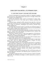
The actual flux path for zero rotor currents when current in phase A is
maximum
2Ii
A
=

and
2/2Iii
CB
−==
, obtained through FEM, is shown in
Figure 5.1. [4]
B
g1max
B
g1

Figure 5.1 No-load flux plot by FEM when i
B
= i
C
= -i
A
/2.
The corresponding radial airgap flux density is shown on Figure 5.1b. In the
absence of slotting and stator mmf harmonics, the airgap field is sinusoidal, with
an amplitude of B
g1max
.
In the presence of slot openings, the fundamental of airgap flux density is
B
g1
. The ratio of the two amplitudes is called the Carter coefficient.

1g
max1g

C
B
B
K =
(5.1)
© 2002 by CRC Press LLC
Author: Ion Boldea, S.A.Nasar………… ………




When the magnetic airgap is not heavily saturated, K
C
may also be written as
the ratio between smooth and slotted airgap magnetic permeances or between a
larger equivalent airgap g
e
and the actual airgap g.

1
g
g
K
e
C
≥=
(5.2)
FEM allows for the calculation of Carter coefficient from (5.1) when it is
applied to smooth and double-slotted structure (Figure 5.1).
On the other hand, easy to handle analytical expressions of K

C
, based on
conformal transformation or flux tube methods, have been traditionally used, in
the absence of saturation, though. First, the airgap is split in the middle and the
two slottings are treated separately. Although many other formulas have been
proposed, we still present Carter’s formula as it is one of the best.

2/g
K
2,1r,s
r,s
2,1C
⋅γ−τ
τ
=
(5.3)
τ
s,r
–stator/rotor slot pitch, g–the actual airgap, and

g
b
25
g
b
2
g
b
1ln
g

b
tan/
g
b
4
r,os
2
r,os
2
r,osr,osr,os
2,1
+








≈



















+−








π
=γ (5.4)
for b
os,r
/g >>1. In general, b
os,r
≈ (3 - 8)g. Where b
os,r
is the stator(rotor) slot
opening.
With a good approximation, the total Carter coefficient for double slotting is

2C1CC
KKK ⋅=
(5.5)
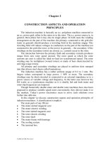
B
gav
b
or
τ
or
B
gmax
B
~
B
gmin

Figure 5.2 Airgap flux density for single slotting
The distribution of airgap flux density for single-sided slotting is shown on
Figure 5.2. Again, the iron permeability is considered to be infinite. As the
© 2002 by CRC Press LLC
Author: Ion Boldea, S.A.Nasar………… ………




magnetic circuit becomes heavily saturated, some of the flux lines touch the slot
bottom (Figure 5.3) and the Carter coefficient formula has to be changed. [2]
In such cases, however, we think that using FEM is the best solution.
If we introduce the relation

maxgmingmaxg~
B2BBB
β=−=
(5.6)
the flux drop (Figure 5.2) due to slotting ∆Φ is

r,s~
r,os
r,s
B
2
b
σ=∆Φ
(5.7)
From [3],
2,1r,os
2
g
b γ=βσ
(5.8)

Figure 5.3 Flux lines in a saturated magnetic circuit
The two factors β and σ are shown on Figure 5.4 as obtained through
conformal transformations. [3]
When single slotting is present, g/2 should be replaced by g.
0.1
0.2
0.3
0.4
0

2 4 6 8 10 12
1.4
1.6
1.8
2.0
β
σ
b /g
os,r

Figure 5.4 The factor β and σ as function of b
os,r
/(g/2)
Another slot-like situation occurs in long stacks when radial channels are
placed for cooling purposes. This problem is approached next.
© 2002 by CRC Press LLC
Author: Ion Boldea, S.A.Nasar………… ………




5.3 EFFECTIVE STACK LENGTH
Actual stator and rotor stacks are not equal in length to avoid notable axial
forces, should any axial displacement of rotor occured. In general, the rotor
stack is longer than the stator stack by a few airgaps (Figure 5.5).

()
g64ll
sr
−+=

(5.9)
stator
rotor
l
r
l
s

Figure 5.5. Single stack of stator and rotor
Flux fringing occurs at stator stack ends. This effect may be accounted for
by apparently increasing the stator stack by (2 to 3)g,

()
g32ll
sse
÷+=
(5.10)
The average stack length, l
av
, is thus

se
rs
av
l
2
ll
l
≈
+

≈
(5.11)
As the stacks are made of radial laminations insulated axially from each
other through an enamel, the magnetic length of the stack L
e
is

Feave
KlL ⋅=
(5.12)
The stacking factor K
Fe
(K
Fe
= 0.9 – 0.95 for (0.35 – 0.5) mm thick
laminations) takes into account the presence of nonmagnetic insulation between
laminations.
b
c
l’

Figure 5.6 Multistack arrangement for radial cooling channels
When radial cooling channels (ducts) are used by dividing the stator into n
elementary ones, the equivalent stator stack length L
e
is (Figure 5.6)
© 2002 by CRC Press LLC
Author: Ion Boldea, S.A.Nasar………… ………

()
g2ng2K'l 1nL
Fee
++⋅+≈
(5.12)
with
mm 250100'l;mm 105b
c
−=−=
(5.13)
It should be noted that recently, with axial cooling, longer single stacks up
to 500mm and more have been successfully built. Still, for induction motors in
the MW power range, radial channels with radial cooling are in favor.
5.4 THE BASIC MAGNETIZATION CURVE
The dependence of airgap flux density fundamental B
g1
on stator mmf
fundamental amplitude F
1m
for zero rotor currents is called the magnetization
curve.
For mild levels of magnetic saturation, usually in general, purpose induction
motors, the stator mmf fundamental produces a sinusoidal distribution of the
flux density in the airgap (slotting is neglected). As shown later in this chapter
by balancing the magnetic saturation of teeth and back cores, rather sinusoidal
airgap flux density is maintained, even for very heavy saturation levels.
The basic magnetization curve (F

1m
(B
g1
) or I
0
(B
g1
) or I
o
/I
n
versus B
g1
) is
very important when designing an induction motor and notably influences the
power factor and the core loss. Notice that I
0
and I
n
are no load and full load
stator phase currents and F
1m0
is

1
01w1
0m1
p
IKW23
F

π
=
(5.14)
The no load (zero rotor current) design airgap flux density is B
g1
= 0.6 –
0.8T for 50 (60) Hz induction motors and goes down to 0.4 to 0.6 T for (400 to
1000) Hz high speed induction motors, to keep core loss within limits.
On the other hand, for 50 (60) Hz motors, I
0
/I
n
(no-load current/rated
current) decreases with motor power from 0.5 to 0.8 (in subkW power range) to
0.2 to 0.3 in the high power range, but it increases with the number of pole
pairs.
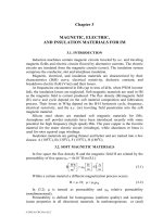
0.1 0.2 0.3 0.4 0.5
0.2
0.4
0.6
0.8
B [T]
g1
p =1,2
p =4-8
I /I
0n
1
1

Figure 5.7 Typical magnetization curves
© 2002 by CRC Press LLC
Author: Ion Boldea, S.A.Nasar………… ………




For low airgap flux densities, the no-load current tends to be smaller. A
typical magnetization curve is shown in Figure 5.7 for motors in the kW power
range at 50 (60) Hz.
Now that we do have a general impression on the magnetising (mag.) curve,
let us present a few analytical methods to calculate it.
5.4.1 The magnetization curve via the basic magnetic circuit
We shall examine first the flux lines corresponding to maximum flux
density in the airgap and assume a sinusoidal variation of the latter along the
pole pitch (Figure 5.8a,b).

() ( )
θ=θω−θ=θ
1e11m1ge1g
p ; tpcosBt,B
(5.15)
For t = 0
()
θ=θ
1m1gg
pcosB0,B
(5.16)
The stator (rotor) back iron flux density B
cs,r

is

()
2
D
dt,B
h2
1
B
0
1g
r,cs
r,cs
⋅θθ=
∫
θ
(5.17)
where h
cs,r
is the back core height in the stator (rotor). For the flux line in Figure
5.8a (θ = 0 to π/p
1
),

() ()
1
11m1g
cs
1cs
p2

D
; tpsinB
h
2
2
1
t,B
π
=τω−θ⋅
τ
π
=θ
(5.18)
30 /p
0
F
equivalent
flux line
F
F
F
F
a.)
cs
ts
tr
cr
g
π2π3π4π
B

cs1
()
θ
B
g1
()
θ
t=0
p
θ
1
b.)
1

Figure 5.8 Flux path a.) and flux density types b.): ideal distribution in the airgap and stator core
© 2002 by CRC Press LLC
Author: Ion Boldea, S.A.Nasar………… ………




Due to mmf and airgap flux density sinusoidal distribution along motor
periphery, it is sufficient to analyse the mmf iron and airgap components F
ts
, F
tr

in teeth, F
g
in the airgap, and F

cs
, F
cr
in the back cores. The total mmf is
represented by F
1m
(peak values).

crcstrtsgm1
FFF2F2F2F2
++++=
(5.19)
Equation (5.19) reflects the application of the magnetic circuit (Ampere’s)
law along the flux line in Figure 5.8a.
In industry, to account for the flattening of the airgap flux density due to
teeth saturation, B
g1m
is replaced by the actual (designed) maximum flattened
flux density B
gm
, at an angle θ = 30°/p
1
, which makes the length of the flux lines
in the back core 2/3 of their maximum length.
Then finally the calculated I
1m
is multiplied by
3/2
(1/cos30°) to find the
maximum mmf fundamental.

At θ
er
= p
1
θ = 30°, it is supposed that the flattened and sinusoidal flux
density are equal to each other (Figure 5.9).
B
g
()
θ
(F)
30
0
1
F
B
B
π
p
θ
1m
g1m
gm

Figure 5.9 Sinusoidal and flat airgap flux density
We have to again write Ampere’s law for this case (interior flux line in
Figure 5.8a).

()
(

)
crcstrtsgmg
30
1
FFF2F2BF2F2
0
++++=
(5.20)
and finally,
()
0
30
1
m1
30cos
F2
F2
0
=
(5.21)
For the sake of generality we will use (5.20) – (5.21), remembering that the
length of average flux line in the back cores is 2/3 of its maximum.
Let us proceed directly with a numerical example by considering an
induction motor with the geometry in Figure 5.10.

T7.0B ;m035.0D ;m018.0h
;m100.5g ;b4.1b ;b2.1b ;18N
;24N ;m025.0h ;m176.0D 0.1m;D ;4p2
gmshaftr
3-

1tss11trr1r
sse1
===
⋅====
=====
(5.22)
© 2002 by CRC Press LLC
Author: Ion Boldea, S.A.Nasar………… ………




60 /p
0
l
h
b
b
D
g
l
h
b
b
b
b
D
shaft
cs
cr

r
s
ts2
ts1
tr1
tr2
r1
s1
e
2P =4
1

Figure 5.10 IM geometry for magnetization curve calculation
The B/H curve of the rotor and stator laminations is given in Table 5.1.
Table 5.1 B/H curve a typical IM lamination
B[T]
0.0 0.05 0.1 0.15 0.2 0.25 0.3 0.35 0.4 0.45 0.5 0.55 0.6
H[A/m]
0 22.8 35 45 49 57 65 70 76 83 90 98 206
B[T]
0.65 0.7 0.75 0.8 0.85 0.9 0.95 1 1.05 1.1 1.15 1.2 1.25
H[A/m]
115 124 135 148 177 198 198 220 237 273 310 356 417
1.3 1.35 1.4 1.45 1.5 1.55 1.6 1.65 1.7
482 585 760 1050 1340 1760 2460 3460 4800
1.75 1.8 1.85 1.9 1.95 2.0
6160 8270 11170 15220 22000 34000

Based on (5.20) – (5.21), Gauss law, and B/H curve in Table 5.1, let us
calculate the value of F

1m
.
To solve the problem in a rather simple way, we still assume a sinusoidal
flux distribution in the back cores, based on the fundamental of the airgap flux
density B
g1m
.

T809.0
3
2
7.0
30cos
B
B
0
gm
m1g
===
(5.23)
The maximum stator and rotor back core flux densities are obtained from
(5.18):

m1g
cs1
csm
B
h
1
p2

D1
B
π
⋅
π
=
(5.24)
© 2002 by CRC Press LLC
Author: Ion Boldea, S.A.Nasar………… ………





m1g
cr1
crm
B
h
1
p2
D1
B
π
⋅
π
=
(5.25)
with
()

m013.0
2
025.02100.0174.0
2
h2DD
h
se
cs
=
⋅−−
=
−−
=
(5.26)

()
m0135.0
2
036.0018.02001.0100.0
2
h2Dg2D
h
rshaft
cr
=
−⋅−−
=
−−−
=

Now from (5.24) – (5.25),

T555.1
013.04
809.01.0
B
csm
=
⋅
⋅
=
(5.28)

T498.1
0135.04
809.01.0
B
crm
=
⋅
⋅
=
(5.29)
As the core flux density varies from the maximum value cosinusoidally, we
may calculate an average value of three points, say B
csm
, B
csm
cos60
0

and
B
csm
cos30
0
:

T285.18266.0555.1
6
30cos60cos41
BB
00
csmcsav
=⋅=








++
=
(5.30)

T238.18266.0498.1
6
30cos60cos41
BB

00
crmcrav
=⋅=








++
=
(5.31)
From Table 5.1 we obtain the magnetic fields corresponding to above flux
densities. Finally, H
csav
(1.285) = 460 A/m and H
crav
(1.238) = 400 A/m.
Now the average length of flux lines in the two back irons are

()()
m0853.0
4
013.0176.0
3
2
p2
hD

3
2
l
1
cse
csav
=
−
π=
−π
⋅≈
(5.32)

()()
m02593.0
4
135.036.0
3
2
p2
hD
3
2
l
1
crshaft
crav
=
+
π=

+π
⋅≈
(5.33)
Consequently, the back core mmfs are

Aturns238.394600853.0HlF
csavcsavcs
=⋅=⋅=
(5.34)

Aturns362.104000259.0HlF
cravcravcr
=⋅=⋅=
(5.35)
The airgap mmf Fg is straightforward.
© 2002 by CRC Press LLC
Author: Ion Boldea, S.A.Nasar………… ………





Aturns324.557
10256.1
7.0
105.02
B
g2F2
6
3

0
gm
g
=
⋅
⋅⋅⋅=
µ
⋅=
−
−
(5.36)
Assuming that all the airgap flux per slot pitch traverses the stator and rotor
teeth, we have

()()
(
)
()
r,tsr,sr,s
r,s
t
av
r,ts
av
r,ts
r,s
gm
b/b1N
hD
b ;bB

N
D
B
r,s
+
±π
=⋅=
π
⋅
(5.37)
Considering that the teeth flux is conserved (it is purely radial), we may
calculate the flux density at the tooth bottom and top as we know the average
tooth flux density for the average tooth width (b
ts,r
)
av
. An average can be applied
here again. For our case, let us consider (B
ts,r
)
av
all over the teeth height to
obtain

()
()
()
()
()
()

m1000.6
182.11
018.01.0
b
m1081.6
244.11
025.01.0
b
3
av
tr
3
av
ts
−
−
⋅=
⋅+
−π
=
⋅=
⋅+
+π
=
(5.38)

()
()
T878.1
1056.618

1007.0
B
T344.1
1043.724
1007.0
B
3
av
tr
3
av
ts
=
⋅⋅
⋅π⋅
=
=
⋅⋅
⋅π⋅
=
−
−
(5.39)
From Table 5.1, the corresponding values of H
tsav
(B
tsav
) and H
trav
(B

trav
) are
found to be H
tsav
= 520 A/m, H
trav
= 13,600 A/m. Now the teeth mmfs are

() ( )
Aturns262025.0520h2HF2
stsavts
=⋅⋅=≈
(5.40)

() ( )
Aturns6.4892018.013600h2HF2
rtravtr
=⋅⋅=≈
(5.41)
The total stator mmf
()
0
30
1
F
is calculated from (5.20)

()
Aturns56.1122362.10238.396.48926324.557F2
0

30
1
=++++=
(5.42)
The mmf amplitude F
m10
(from 5.21) is

()
Aturns764.1297
3
2
56.1122
30cos
F2
F2
0
30
1
0m1
0
=⋅==
(5.43)
Based on (5.14), the no-load current may be calculated with the number of
turns/phase W
1
and the stator winding factor K
w1
already known.
Varying as the value of B

gm
desired the magnetization curve–B
gm
(F
1m
)–is
obtained.
© 2002 by CRC Press LLC
Author: Ion Boldea, S.A.Nasar………… ………




Before leaving this subject let us remember the numerous approximations
we operated with and define two partial and one equivalent saturation factor as
K
st
, K
sc
, K
s
.

() ()
g
crcs
sc
g
trts
st

F2
FF
1K ;
F2
FF2
1K
+
+=
+
+=
(5.44)

()
1KK
F2
F
K
scst
g
30
1
s
0
−+== (5.45)
The total saturation factor K
s
accounts for all iron mmfs as divided by the
airgap mmf. Consequently, we may consider the presence of iron as an
increased airgap g
es

.









==
n
0
sssces
I
I
KK ;KgKg
(5.46)
Let us notice that in our case,

103.21089.1925.1K
089.1
324.557
362.1023.39
1K ; 925.1
324.557
6.48926
1K
s
ctst

=−+=
=
+
+==
+
+=
(5.47)
A few remarks are in order.
• The teeth saturation factor K
st
is notable while the core saturation factor is
low; so the tooth are much more saturated (especially in the rotor, in our
case); as shown later in this chapter, this is consistent with the flattened
airgap flux density.
• In a rather proper design, the teeth and core saturation factors K
st
and K
sc

are close to each other: K
st
≈ K
sc
; in this case both the airgap and core flux
densities remain rather sinusoidal even if rather high levels of saturation are
encountered.
• In 2 pole machines, however, K
sc
tends to be higher than K
st

as the back
core height tends to be large (large pole pitch) and its reduction in size is
required to reduce motor weight.
• In mildly saturated IMs, the total saturation factor is smaller than in our
case: K
s
= 1.3 – 1.6.
Based on the above theory, iterative methods, to obtain the airgap flux
density distribution and its departure from a sinusoid (for a sinusoidal core flux
density), have been recently introduced [2,4]. However, the radial flux density
components in the back cores are still neglected.



© 2002 by CRC Press LLC
Author: Ion Boldea, S.A.Nasar………… ………




5.4.2 Teeth defluxing by slots
So far we did assume that all the flux per slot pitch goes radially through the
teeth. Especially with heavily saturated teeth, a good part of magnetic path
passes through the slot itself. Thus, the tooth is slightly “discharged” of flux.
We may consider that the following are approximates:

0.1c ;b/bBcBB
1r,tsr,sg1tit
<<−=
(5.48)

r,ts
r,sr,ts
gti
b
bb
BB
+
=
(5.49)
The coefficient c
1
is, in general, adopted from experience but it is strongly
dependent on the flux density in the teeth B
ti
and the slotting geometry
(including slot depth [2]).
5.4.3 Third harmonic flux modulation due to saturation
As only inferred above, heavy saturation in stator (rotor) teeth and/or back
cores tends to flatten or peak, respectively, the airgap flux distribution.
This proposition can be demonstrated by noting that the back core flux
density B
cs,r
is related to airgap (implicitly teeth) flux density by the equation

()
θ=θθθ=
∫
θ
1er

0
ererr,tsr,sr,cs
p ;dBCB
er
(5.50)
π
/2
π
teeth
B
t1
relative
flux
density
θ
er
B
t3
core
B
B
c1
c3
π
/2
π
θ
er
B >0
ts,r

π
/2
π
teeth
B
t1
relative
flux
density
θ
er
B
t3
core
B
B
c1
c3
π
/2
π
θ
er
B <0
ts,r

Figure 5.11 Tooth and core flux density distribution
a.) saturated back core (B
ts,r3
> 0); b.) saturated teeth (B

ts,r3
< 0)
Magnetic saturation in the teeth means flattening B
ts,r
(θ) curve.

(
)
(
)
(
)
t3cosBtcosBB
1er3r,ts1er1r,tsr,ts
ω−θ+ω−θ=θ
(5.51)
© 2002 by CRC Press LLC
Author: Ion Boldea, S.A.Nasar………… ………




Consequently, B
ts,r3
> 0 means unsaturated teeth (peaked flux density,
Figure 5.11a). With (5.51), equation (5.50) becomes

() ()







ω−θ+ω−θ= t3sin
3
B
tsinBCB
1er
3r,ts
1er1r,tsr,sr,cs
(5.52)
Analyzing Figure 5.11, based on (5.51) – (5.52), leads to remarks such as
• Oversaturation of a domain (teeth or core) means flattened flux density in
that domain (Figure 5.11b).
• In paragraph 5.4.1. we have considered flattened airgap flux density–that is
also flattened tooth flux density–and thus oversaturated teeth is the case
treated.
• The flattened flux density in the teeth (Figure 5.11b) leads to only a slightly
peaked core flux density as the denominator 3 occurs in the second term of
(5.52).
• On the contrary, a peaked teeth flux density (Figure 5.11a) leads to a flat
core density. The back core is now oversaturated.
• We should also mention that the phase connection is important in third
harmonic flux modulation. For sinusoidal voltage supply and delta
connection, the third harmonic of flux (and its induced voltage) cannot
exist, while it can for star connection. This phenomenon will also have
consequences in the phase current waveforms for the two connections.
Finally, the saturation produced third and other harmonics influence,
notably the core loss in the machine. This aspect will be discussed in

Chapter 11 dedicated to losses.
After describing some aspects of saturation – caused distribution
modulation, let us present a more complete analytical nonlinear field model,
which also allows for the calculation of actual spatial flux density distribution in
the airgap, though with smoothed airgap.
5.4.4 The analytical iterative model (AIM)
Let us remind here that essentially only FEM [5] or extended magnetic
circuit methods (EMCM) [6] are able to produce a rather fully realistic field
distribution in the induction machine. However, they do so with large
computation efforts and may be used for design refinements rather than for
preliminary or direct optimization design algorithms.
A fast analytical iterative (nonlinear) model (AIM) [7] is introduced here
for preliminary or optimization design uses.
The following assumptions are introduced: only the fundamental of m.m.f.
distribution is considered; the stator and rotor currents are symmetric; - the IM
cross-section is divided into five circular domains (Figure 5.12) with unique
(but adjustable) magnetic permeabilities essentially distinct along radial (r) and
tangential (θ) directions: µ
r
, and µ
0
; the magnetic vector potential A lays along
the shaft direction and thus the model is two-dimensional; furthermore, the
separation of variables is performed.
© 2002 by CRC Press LLC
Author: Ion Boldea, S.A.Nasar………… ………

Magnetic potential, A, solution

Figure 5.12 The IM cross-section divided into five domains
The Poisson equation in polar coordinates for magnetic potential A writes

J
A
r
11
r
A
r
A
r
11
2
2
2
r
2
2
−=
θ∂
∂
µ
+









∂
∂
+
∂
∂
µ
θ
(5.53)
Separating the variables, we obtain
A(r,θ) = R(r) ⋅ T(θ) (5.54)
Now, for the domains with zero current (D
1
, D
3
, D
5
) – J = O, Equation
(5.53) with (5.54) yields

()
() ()
()
()
2
2
22

2
2
2
2
d
Td
T
;
dr
rRd
r
dr
rdR
r
rR
1
λ−=
θ
θ
θ
α
λ=









+
(5.55)
© 2002 by CRC Press LLC
Author: Ion Boldea, S.A.Nasar………… ………




with α
2
= µ
θ
/µ
r
and λ a constant.
Also a harmonic distribution along
θ
direction was assumed. From (5.55):

() ()
0R
dr
rdR
r
dr
rRd
r
2
2
2

2
=λ−+ (5.56)
and
()
0T
d
Td
2
2
2
2
=
α
λ
+
θ
θ
(5.57)
The solutions of (5.56) and (5.57) are of the form

()
λ−λ
+= rCrCrR
21
(5.58)

()







θ
α
λ
+






θ
α
λ
=θ
sinCcosCT
43
(5.59)
as long as r ≠ 0.
Assuming further symmetric windings and currents, the magnetic potential
is an aperiodic function and thus,
A(r,0) = 0 (5.60)

0
p
,rA
1
=









π
(5.61)
Consequently, from (5.59), (5.57) and (5.53), A(r,θ) is

()
()
()
θ⋅+⋅=θ
α−α
1
pp
psinrhrg,rA
11
(5.62)
Now, if the domain contains a homogenous current density J,

()
θ=
1m
psinJJ
(5.63)
the particular solution A

p
(r,θ) of (5.54) is:

() ()
θ=θ
1
2
p
PsinKr,rA
(5.64)
with
m
2
1r
r
J
p4
K
θ
θ
µ−µ
µµ
−=
(5.65)
Finally, the general solution of A (5.53) is

()
()
()
θ+⋅+⋅=θ

α−α
1
2
pp
psinKrrhrg,rA
11
(5.66)
As (5.66) is valid for homogenous media, we have to homogenize the
slotting domains D
2
and D
4
, as the rotor and stator yokes (D
1
, D
5
) and the airgap
(D
3
) are homogenous.
© 2002 by CRC Press LLC
Author: Ion Boldea, S.A.Nasar………… ………




Homogenizing the Slotting Domains.
The main practical slot geometries (Figure 5.13) are defined by equivalent
center angles θ
s

, and θ
t
, for an equivalent (defined) radius r
m4
, (for the stator)
and r
m2
(for the rotor). Assuming that the radial magnetic field H is constant
along the circles r
m2
and r
m4
, the flux linkage equivalence between the
homogenized and slotting areas yields

()
1xstr1xs01xtt
Lr HLrHLrH θ+θµ=θµ+θµ
(5.67)
Consequently, the equivalent radial permeability µ
r
, is

st
s0tt
r
θ+θ
θµ+θµ
=µ
(5.68)

For the tangential field, the magnetic voltage relationship (along A, B, C
trajectory on Figure 5.13), is

mBCmABmAC
VVV +=
(5.69)

Figure 5.13 Stator and rotor slotting
With B
θ
the same, we obtain

()
xs
0
xt
t
xst
r
B
r
B
r
B
θ
µ
+θ
µ
=θ+θ
µ

θθ
θ
θ
(5.70)
© 2002 by CRC Press LLC
Author: Ion Boldea, S.A.Nasar………… ………




Consequently,

()
stt0
st0t
θµ+θµ
θ+θµµ
=µ
θ
(5.71)
Thus the slotting domains are homogenized to be characterized by distinct
permeabilities µ
r
, and µ
θ
along the radial and tangential directions, respectively.
We may now summarize the magnetic potential expressions for the five
domains:

()

()
()
()
()
()
()
()
()
()
()
()
()
()
()
erd ;psinrkrhrg,rA
crb ;psinrkrhrg,rA
fre ;psinrhrg,rA
drc ;psinrhrg,rA
br
2
a
a' ;psinrhrg,rA
1
2
4
p
4
p
44
1

2
2
p
2
p
22
1
p
5
p
55
1
p
3
p
33
1
p
1
p
11
4141
2121
11
11
11
<<θ++=θ
<<θ++=θ
<<θ+=θ
<<θ+=θ

<<=θ+=θ
α−α
α−α
−
−
−
(5.72)
with
2m
2
2
12r
22r
2
4m
4
2
14r
44r
4
J
p4
K
J
p4
K
θ
θ
θ
θ

µ−µ
µµ
+=
µ−µ
µµ
−=
(5.73)
J
m2
represents the equivalent demagnetising rotor equivalent current density
which justifies the ⊕ sign in the second equation of (5.73). From geometrical
considerations, J
m2
and J
m4
are related to the reactive stator and rotor phase
currents I
1s
and I
2r
′, by the expressions (for the three-phase motor),

s11w1
22
4m
r21w1
22
2m
IKW
de

126
J
'IKW
bc
126
J
−π
=
−π
=
(5.74)
The main pole-flux-linkage Ψ
m1
is obtained through the line integral of A
3

around a pole contour Γ (L
1
, the stack length):









π
==ψ

∫
Γ
1
31
3
1m
P2
,dAL2dlA
(5.75)
Notice that A
3
(d, π/2p
1
,) = −A
3
(d,– π/2p
1
,) because of symmetry. With A
3
from
(5.72), ψ
m1
becomes

()
11
p
3
p
311m

dhdgL2
−
+=ψ
(5.76)
Finally, the e.m.f. E
1
, (RMS value) is
© 2002 by CRC Press LLC
Author: Ion Boldea, S.A.Nasar………… ………





1m1w111
KWf2E ψπ=
(5.77)
Now from boundary conditions, the integration constants g
i
and h
i
are
calculated as shown in the appendix of [7].
The computer program
To prepare the computer program, we have to specify a few very important
details. First, instead of a (the shaft radius), the first domain starts at a′=a/2 to
account for the shaft field for the case when the rotor laminations are placed
directly on the shaft. Further, each domain is characterized by an equivalent (but
adjustable) magnetic permeability. Here we define it. For the rotor and stator
domains D

1
, and D
5
, the equivalent permeability would correspond to r
m1
=
(a+b)/2 and r
m5
= (e+f)/2, and tangential flux density (and θ
0
= π/4).

()
()
4
sin
2
fe
h
2
fe
gp,rB
4
sin
2
ba
h
2
ba
gp,rB

1p
5
1p
5105m5
1p
1
1p
1101m1
11
11
π














+
−







+
−=θ
π














+
−






+
−=θ

−−−
θ
−−−
θ
(5.78)
For the slotting domains D
2
and D
4
, the equivalent magnetic permeabilities
correspond to the radiuses r
m2
and r
m4
(Figure 5.13) and the radial flux densities
B
2r
, and B
4r
.

(
)
(
)
()
()
014m4
1p
4m4

1p
4m4104mr4
012m2
1p
2m2
1p
2m2102mr2
pcosrKrhrgp,rB
pcosrKrhrgp,rB
4141
2121
θ++=θ
θ++=θ
−α−−α
−α−−α
(5.79)
with cosP
1
θ
0
= 0.9 … 0.95. Now to keep track of the actual saturation level, the
actual tooth flux densities B
4t
, and B
2t
, corresponding to B
2r
, H
2r
and B

4r
, H
4r
are

r40
4t
4s
0r4
4t
4s4t
t4
r20
2t
2s
0r2
2t
2s1t
t2
HcBB
HcBB
µ
θ
θ
−
θ
θ+θ
=
µ
θ

θ
−
θ
θ+θ
=
(5.80)
The empirical coefficient c
0
takes into account the tooth magnetic unloading due
to the slot flux density contribution.
Finally, the computing algorithm is shown on Figure 5.14 and starts with
initial equivalent permeabilities.
For the next cycle of computation, each permeability is changed according
to

() () () ()
(
)
i1i
1
i1i
c
µ−µ+µ=µ
++
(5.81)
It has been proved that c
1
= 0.3 is an adequate value, for a wide power range.
© 2002 by CRC Press LLC
Author: Ion Boldea, S.A.Nasar………… ………

Figure 5.14 The computation algorithm
Model validation on no-load
The AIM has been applied to 12 different three-phase IMs from 0.75 kW to
15 kW (two-pole and four-pole motors), to calculate both the magnetization
curve I
10
= f(E
1
) and the core losses on no load for various voltage levels.
The magnetizing current is I
µ

= I
1r
and the no load active current I
0A
is
© 2002 by CRC Press LLC
Author: Ion Boldea, S.A.Nasar………… ………





0

coppermvFe
A0
V3
PPP
I
++
=
(5.82)
The no-load current I
10
is thus

2
A0
2
10
III
+=
µ
(5.83)
and
101101
ILVE
σ
ω−≈
(5.84)
where L
1σ
is the stator leakage inductance (known). Complete expressions of
leakage inductances are introduced in Chapter 6.

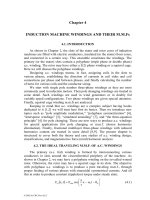
Figure 5.15 exhibits computation results obtained with the conventional
nonlinear model, the proposed model, and experimental data.


Figure 5.15 Magnetization characteristic validation on no load
1. conventional nonlinear model (paragraph 5.4.1); 2. AIM; 3. experiments

© 2002 by CRC Press LLC
Author: Ion Boldea, S.A.Nasar………… ………







Figure 5.15 (continued)
© 2002 by CRC Press LLC
Author: Ion Boldea, S.A.Nasar………… ………





Figure 5.15 (continued)
It seems clear that AIM produces very good agreement with experiments
even for high saturation levels.

A few remarks on AIM seem in order.
• The slotting is only globally accounted for by defining different tangential

and radial permeabilities in the stator and rotor teeth.
• A single, but variable, permeability characterizes each of the machine
domains (teeth and back cores).
• AIM is a bi-directional field approach and thus both radial and tangential
flux density components are calculated.
• Provided the rotor equivalent current I
r
(RMS value and phase shift with
respect to stator current) is given, AIM allows calculation of the
distribution of main flux in the machine on load.
• Heavy saturation levels (V
0
/V
n
> 1) are handled satisfactorily by AIM.
•
By skewing the stack axially, the effect of skewing on main flux
distribution can be handled.
• The computation effort is minimal (a few seconds per run on a
contemporary PC).

So far AIM was used considering that the spatial field distribution is
sinusoidal along stator bore. In reality, it may depart from this situation as
shown in the previous paragraph. We may repeatedly use AIM to produce the
actual spatial flux distribution or the airgap flux harmonics.
AIM may be used to calculate saturation-caused harmonics. The total mmf
F
1m
is still considered sinusoidal (Figure 5.16).
The maximum airgap flux density B

g1m
(sinusoidal in nature) is considered
known by using AIM for given stator (and eventually also rotor) current RMS
values and phase shifts.
By repeatedly using the Ampere’s law on contours such as those in Figure
5.17 at different position θ, we may find the actual distribution of airgap flux
density, by admitting that the tangential flux density in the back core retains the
© 2002 by CRC Press LLC
Author: Ion Boldea, S.A.Nasar………… ………




sinusoidal distribution along θ. This assumption is not, in general, far from
reality as was shown in paragraph 5.4.3.
Ampere’s law on contour Γ (Figure 5.17) is

()
θ=θθ=
∫∫
θ
θ−Γ
1m1
P
P
11m1
pcosF2pdpsinFdlH
1
1
(5.85)

The left side of (5.85) may be broken into various parts (Figure 5.17). It
may easily be shown that, due to the absence of any mmf within contours
ABB′B′′A′′A′A and DCC′′D′′,

∫∫∫∫
==
"CC"C"CDD"AA"A"B"A'ABB
dlHdlH ;dlHdlH
(5.86)

Figure 5.16 Ampere’s law contours
© 2002 by CRC Press LLC
Author: Ion Boldea, S.A.Nasar………… ………





Figure 5.17 Mmf–total and back core component F
We may now divide the mmf components into two categories: those that depend
directly on the airgap flux density B
g
(θ) and those that do not (Figure 5.17).

() () ()
θ+θ+θ=
+ trtsggt
F2F2F2F2
(5.87)

() () ()
θ+θ=θ
crcsc
FFF
(5.88)
Also, the airgap mmf F
g
(
θ
) is

() ()
θ
µ
=θ
g
0
c
g
B
gK
F
(5.89)
Suppose we know the maximum value of the stator core flux density, for
given F
1m
, as obtained from AIM, Bcsm,

()
θ=θ

1csmcs
psinBB
(5.90)
We may now calculate F
cs
(θ) as

() ( )
[]
∫
π
θ
αα=θ
2/
p
csmcscs
1
edsinBH2F
(5.91)
The rotor core maximum flux density Bcrm is also known from AIM for the
same mmf F1m. The rotor core mmf F
cr
(θ) is thus

() ( )
[]
∫
π
θ
αα=θ

2/
p
crmcrcr
1
bdsinBH2F
(5.92)
© 2002 by CRC Press LLC