the induction machine handbook chuong (12)

Chapter 12
THERMAL MODELING AND COOLING
12.1. INTRODUCTION
Besides electromagnetic, mechanical and thermal designs are equally
important.
Thermal modeling of an electric machine is in fact more nonlinear than
electromagnetic modeling. Any electric machine design is highly thermally
constrained.
The heat transfer in an induction motor depends on the level and location of
losses, machine geometry, and the method of cooling.
Electric machines work in environments with temperatures varied, say from
–20
0
C to 50
0
C, or from 20
0
to 100
0
in special applications.
The thermal design should make sure that the motor windings temperatures
do not exceed the limit for the pertinent insulation class, in the worst situation.
Heat removal and the temperature distribution within the induction motor are
the two major objectives of thermal design. Finding the highest winding
temperature spots is crucial to insulation (and machine) working life.
The maximum winding temperatures in relation to insulation classes shown
in Table 12.1.
Table 12.1. Insulation classes
Insulation class Typical winding temperature limit [
0
C]

Class A 105
Class B 130
Class F 155
Class H 180
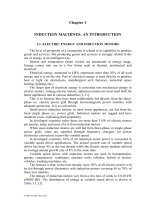
Practice has shown that increasing the winding temperature over the
insulation class limit reduces the insulation life L versus its value L
0
at the
insulation class temperature (Figure 12.1).

T
b
aLLog
+≈
(12.1)
It is very important to set the maximum winding temperature as a design
constraint. The highest temperature spot is usually located in the stator end
connections. The rotor cage bars experience a larger temperature, but they are
not, in general, insulated from the rotor core. If they are, the maximum
(insulation class dependent) rotor cage temperature also has to be observed.
The thermal modeling depends essentially on the cooling approach.
© 2002 by CRC Press LLC© 2002 by CRC Press LLC
Author: Ion Boldea, S.A.Nasar………… ………





Figure 12.1 Insulation life versus temperature rise
12.2. SOME AIR COOLING METHODS FOR IMs

For induction motors, there are four main classes of cooling systems
• Totally enclosed design with natural (zero air speed) ventilation
(TENV)
• Drip-proof axial internal cooling
• Drip-proof radial internal cooling
• Drip-proof radial-axial cooling
In general, fan air-cooling is typical for induction motors. Only for very
large powers is a second heat exchange medium (forced air or liquid) used in the
stator to transfer the heat to the ambient.
TENV induction motors are typical for special servos to be mounted on
machine tools etc., where limited space is available. It is also common for some
static power converter-fed IMs, that operate at large loads for extended periods
of time at low speeds to have an external ventilator running at constant speed to
maintain high cooling in all conditions.
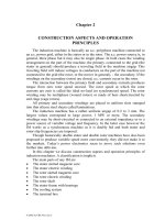
The totally enclosed motor cooling system with external ventilator only
(Figure 12.2b) has been extended lately to hundreds of kW by using finned
stator frames.
Radial and radial-axial cooling systems (Figure 12.2c, d) are in favor for
medium and large powers.
© 2002 by CRC Press LLC
Author: Ion Boldea, S.A.Nasar………… ………




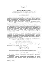
However, axial cooling with internal ventilator and rotor, stator axial
channels in the core, and special rotor slots seem to gain ground for very large
power as it allows lower rotor diameter and, finally, greater efficiency is
obtained, especially with two pole motors (Figure 12.3). [2]
a.)

zero air speed
smooth frame
end ring vents
b.)
finned frame
external
ventilator
internal ventilator

c.
)
d.
)

Figure 12.2 Cooling methods for induction machines
a.) totally enclosed naturally ventilated (TENV);
b.) totally enclosed motor with internal and external ventilator
c.) radially cooled IM d.) radial – axial cooling system
The rotor slots are provided with axial channels to facilitate a kind of direct
cooling.
© 2002 by CRC Press LLC
Author: Ion Boldea, S.A.Nasar………… ………




axial channel
internal ventilator
axial rotor channel
axial rotor cooling

channel
rotor slots

Figure. 12.3 Axial cooling of large IMs
The rather complex (anisotropic) structure of the IM for all cooling systems
presented in Figures 12.2 and 12.3 suggests that the thermal modeling has to be
rather difficult to build.
There are thermal circuit models and distributed (FEM) models. Thermal
circuit models are similar to electric circuits and they may be used both for
thermal steady state and transients. They are less precise but easy to handle and
require a smaller computation effort. In contrast, distributed (FEM) models are
more precise but require large amounts of computation time.
We will define first the elements of thermal circuits based on the three basic
methods of heat transfer: conduction, convection and radiation.
12.3. CONDUCTION HEAT TRANSFER
Heat transfer is related to thermal energy flow from a heat source to a heat
sink.
In electric (induction) machines, the thermal energy flows from the
windings in slots to laminated core teeth through the conductor insulation and
slot line insulation.
On the other hand, part of the thermal energy in the end-connection
windings is transferred through thermal conduction through the conductors
axially toward the winding part in slots. A similar heat flow through thermal
conduction takes place in the rotor cage and end rings.
There is also thermal conduction from the stator core to the frame through
the back core iron region and from rotor cage to rotor core, respectively, to shaft
and axially along the shaft. Part of the conduction heat now flows through the
slot insulation to core to be directed axially through the laminated core. The
presence of lamination insulation layers will make the thermal conduction along
the axial direction more difficult. In long stack IMs, axial temperature

differentials of a few degrees (less than 10
0
C in general), (Figure 12.4), occur.
© 2002 by CRC Press LLC
Author: Ion Boldea, S.A.Nasar………… ………




circumpherential
flow
shaft
rotor
core
radial
flow
stator
core
stator frame

Figure 12.4 Heat conduction flow routs in the IM
So, to a first approximation, the axial heat flow may be neglected.
Second, after accounting for conduction heat flow from windings in slots to
the core teeth, the machine circumferential symmetry makes possible the
neglecting of circumferential temperature variation.
So we end up with a one-dimensional temperature variation, along the
radial direction. For this crude approximation defining thermal conduction,
convection, and radiation, and of the equivalent circuit becomes a rather simple
task.
The Fourier’s law of conduction may be written, for steady state, as

()
qK =θ∆−∇
(12.2)
where q is heat generation rate per unit volume (W/m
3
); K is thermal
conductivity (W/m,
0
C) and θ is local temperature.
For one-dimensional heat conduction, Equation (12.2), with constant
thermal conductivity K, becomes:

q
x
K
2
2
=
∂
θ∂
−
(12.3)
A basic heat conduction element (Figure 12.5) shows that power Q
transported along distance l of cross section A is

AlqQ ⋅⋅≈
(12.4)
with q, A – constant along distance l.
The thermal conduction resistance R

con
may be defined as similar to
electrical resistance.

[]
W/C
KA
l
R
0
con
=
(12.5)
© 2002 by CRC Press LLC
Author: Ion Boldea, S.A.Nasar………… ………




Area A
Q
2
Q
Q
1
x=0
θ=θ
1
x=l
θ=θ

2
l
stack
b
h
s
s
∆
ins
fA

Figure 12.5 One dimensional heat conduction
Temperature takes the place of voltage and power (losses) replaces the
electrical current.
For a short l, the Fourier’s law in differential form yields

[]
2
W/mdensity flowheat f ;
x
Kf −
∆
θ∆
−≈
(12.6)
If the heat source is in a thin layer,

A
p
f

cos
=
(12.7)
p
cos
in watts is the electric power producing losses and A the cross-section area.
For the heat conduction through slot insulation
∆
ins
(total, including all
conductor insulation layers from the slot middle (Figure 12.5)), the conduction
area A is

(
)
stator/slotsN ;Nlbh2A
ssstackss
−+=
(12.8)
The temperature differential between winding in slots and the core teeth
∆θ
Co
is

AK
R ;Rp
ins
conconcosCos
∆
==θ∆

(12.9)
In well-designed IMs, ∆Θ
cos
< 10
0
C with notably smaller values for small
power induction motors.
The improvement of insulation materials in terms of thermal conductivity
and in thickness reduction have been decisive factors in reducing the slot
insulation conductor temperature differential. Thermal conductivity varies with
temperature and is constant only to a first approximation. Typical values are
given in Table 12.2. The low axial thermal conductivity of the laminated cores
is evident.

© 2002 by CRC Press LLC
Author: Ion Boldea, S.A.Nasar………… ………




Table 12.2. Thermal conductivity
Material Thermal conductivity
(W/m
0
C)
Specific heat coefficient C
s

(J/Kg/
0

C)
Copper 383 380
Aluminum
Carbonsteel
204
45
900
Motor grade steel 23 500
Si steel lamination
– Radial;
– Axial

20 – 30
2.0
490
Micasheet 0.43 -
Varnished cambric 2.0 -
Press board Normex 0.13 -
12.4. CONVECTION HEAT TRANSFER
Convection heat transfer takes place between the surface of a solid body
(the stator frame) and a fluid (air, for example) by the movement of the fluid.
The temperature of a fluid (air) in contact with a hotter solid body rises and
sets a fluid circulation and thus heat transfer to the fluid occurs.
The heat flow out of a body by convection is

θ∆= hAq
conv
(12.10)
where A is the solid body area in contact with the fluid; ∆θ is the temperature
differential between the solid body and bulk of the fluid, and h is the convection

heat coefficient (W/m
2
⋅
0
C).
The convection heat transfer coefficient depends on the velocity of the
fluid, fluid properties (viscosity, density, thermal conductivity), the solid body
geometry, and orientation. For free convention (zero forced air speed and
smooth solid body surface [2])

()
(
)
()
(
)
()
(
)
Cm W/- horizontal 67.0h
Cm W/-down l vertica496.0h
Cm W/- up l vertica158.2h
0
2
25.0
Co
0
2
25.0
Co

0
2
25.0
Co
θ∆≈
θ∆≈
θ∆≈
(12.11)
where ∆θ is the temperature differential between the solid body and the fluid.
For ∆θ = 20
0
C (stator frame θ
1
= 60
0
C, ambient temperature θ
2
= 40
0
C) and
vertical – up surface

()
(
)
CmW/5.44060158.2h
0
2
25.0
Co

=−=
When air is blown with a speed U along the solid surfaces, the convection
heat transfer coefficient h
c
is

()
(
)
UK1huh
Co
0
C
+= (12.12)
© 2002 by CRC Press LLC
Author: Ion Boldea, S.A.Nasar………… ………




with K = 1.3 for perfect air blown surface; K = 1.0 for the winding end
connection surface, K = 0.8 for the active surface of rotor, K = 0.5 for the
external stator frame.
Alternatively,

()
(
)
5m/sfor U Cm W/
L

U
77.1uh
0
2
25.0
75.0
C
>=
(12.13)
U in m/s and L is the length of surface in m.
For a closed air blowed surface – inside the machine:

()
()
()
a
air
Co
c
C
a ;2/a1UK1hUh
θ
θ
=−+=
(12.14)
θ
air
–local air heating; θ
a
–heating (temperature) of solid surface.

In general, θ
air
= 35 – 40
0
C while θ
a
varies with machine insulation class.
So, in general, a < 1.
For convection heat transfer coefficient in axial channels of length, L
(12.13) is to be used.
In radial cooling channels, h
c
c
(U) does not depend on the channel’s length,
but only on speed.

()
(
)
Cm/WU11.23Uh
0
275.0
c
c
≈
(12.15)
12.5. HEAT TRANSFER BY RADIATION
Between two bodies at different temperatures there is a heat transfer by
radiation. One body radiates heat and the other absorbs heat. Bodies which do
not reflect heat, but absorb it, are called black bodies.

Energy radiated from a body with emissivity ε to black surroundings is

()()()()
21
2
2
2
121
4
2
4
1rad
AAq θ−θθ+θθ+θσε=θ−θσε=
(12.16)
σ–Boltzmann’s constant: σ = 5.67⋅10
-8
W/(m
2
K
4
); ε – emissivity; for a black
painted body ε = 0.9; A–radiation area.
In general, for IMs, the radiated energy is much smaller than the energy
transferred by convection except for totally enclosed natural ventilation (TENV)
or for class F(H) motor with very hot frame (120 to 150°C).
For the case when θ
2
= 40° and θ
1
= 80°C, 90°C, 100°C, ε = 0.9, h

rad
= 7.67,
8.01, and 8.52 W/(m
2
°C).
For TENV with h
Co
= 4.56 W/(m
2
,

°C) (convection) the radiation is superior
to convection and thus it cannot be neglected. The total (equivalent) convection
coefficient
h
(c+r)0
= h
Co
+ h
rad
≥ 12 W/(m
2
,

°C).
The convection and radiation combined coefficients h
(c+r)0
≈ 14.2W/(m
2
,

°C)
for steel unsmoothed frames, h
(c+r)0
= 16.7W/(m
2
,

°
C) for steel smoothed frames,
© 2002 by CRC Press LLC
Author: Ion Boldea, S.A.Nasar………… ………




h
(c+r)0
= 13.3W/(m
2
,

°C) for copper/aluminum or lacquered or impregnated
copper windings. In practice, for design purposes, this value of h
Co
, which
enters Equations (12.12 through 12.14), is, in fact, h
(c+r)0
, the combined
convection radiation coefficient.

It is well understood that the heat transfer is three dimensional and as K, h
c

and h
rad
are not constants, the heat flow, even under thermal steady state, is a
very complex problem. Before advancing to more complex aspects of heat flow,
let us work out a simple example.

Example 12.1. One – dimensional simplified heat transfer
In an induction motor with p
Co1
= 500 W, p
Co2
= 400 W, p
iron
= 300 W, the
stator slot perimeter 2h
s
+ b
s
= (2.25 + 8) mm, 36 stator slots, stack length: l
stack

= 0.15 m, an external frame diameter D
e
= 0.30 m, finned area frame (4 to 1 area
increase by fins), frame length 0.30m, let us calculate the winding in slots
temperature and the frame temperature, if the air temperature increase around
the machine is 10°C over the ambient temperature of 30°C and the slot

insulation total thickness is 0.8 mm. The ventilator is used and the end
connection/coil length is 0.4.

Solution
First, the temperature differential of the windings in slots has to be
calculated. We assume here that all rotor heat losses crosses the airgap and it
flows through the stator core toward the stator frame.
In this case, the stator winding in slot temperature differential is (12.3)

()
C 83.3
15.0058.036.00.2
6.0500108.0
lbh2NK
l
l
1p
0
3
stacksssins
coil
endcon
1Coins
cos
=
⋅⋅⋅
⋅⋅⋅
=
+









−∆
=θ∆
−

Now we consider that stator winding in slot losses, rotor cage losses, and
stator core losses produce heat that flows radially through stator core by
conduction without temperature differential (infinite conduction!).
Then all these losses are transferred to ambient through the motor frame
through combined free convection and radiation.

()
()
()
C 758.74
1/43.030.02.14
300400500
Ah
q
0
frame0rc
total
aircore
=

⋅⋅⋅π⋅
++
==θ−θ
+

with θ
air
= 40°, θ
ambient
= 30°, the frame (core) temperature θ
core
= 40 + 74.758 =
114.758
°
C and the winding in slots temperature
θ
cos
=
θ
core
+
∆θ
cos
= 114.758 +
3.83 = 118.58°C. In such TENV induction machines, the unventilated stator
winding end turns are likely to experience the highest temperature spot.
However, it is not at all simple to calculate the end connection temperature
distribution.
© 2002 by CRC Press LLC
Author: Ion Boldea, S.A.Nasar………… ………

12.6. HEAT TRANSPORT (THERMAL TRANSIENTS) IN
A HOMOGENOUS BODY
Although the IM is not a homogenous body, let us consider the case of a
homogenous body – where temperature is the same all over.
The temperature of such a body varies in time if the heat produced inside,
by losses in the induction motor, is applied at a certain point in time–as after
starting the motor. The heat balance equation is

()
()
radiation ,conduction ,convectionthrough
body thefrom transfer heat
0
)conv(
cond
body in the
onaccumulati heat
0
t
in W time
unitper
losses
loss
TThA
dt
TTd

McP −+
−
=
(12.17)
M–body mass (in Kg), c
t
–specific heat coefficient (J/(Kg⋅
0
C))
A–area of heat transfer from (to) the body
h–heat transfer coefficient
Denoting by







===
KA
l
R;
Ah
1
R and McC
cond
(rad)
convtt
(12.18)

equation (12.17) becomes

()()
t
00
tloss
R
TT
dt
TTd
CP
−
+
−
=
(12.19)
This is similar to a R
t
, C
t
parallel electric circuit fed from a current source
P
loss
with a voltage T – T
0
(Figure 12.6).
p
loss
R
C

T
T
0
tt
τ
=C R
t
tt
T -T
max
0
T-T
0
t

Figure 12.6 Equivalent thermal circuit
For steady state, C
t
does not enter Equation (12.17) and the equivalent
circuit (Figure 12.6).
The solution of this electric circuit is evident.

()
tt
t
0
t
0max
eTe1TTT
τ

−
τ
−
+








−−=
(12.20)
© 2002 by CRC Press LLC
Author: Ion Boldea, S.A.Nasar………… ………




The thermal time constant τ
t
= C
t
R
t
is very important as it limits the
machine working time with a certain level of losses and given cooling
conditions. Intermittent operation, however, allows for more losses (more
power) for the same given maximum temperature, T

max
.
The thermal time constant increases with machine size and effectivity of the
cooling system. A TENV motor is expected to have a smaller thermal time
constant than a constant speed ventilator-cooled configuration.
12.7. INDUCTION MOTOR THERMAL TRANSIENTS AT STALL
The IM at stall is characterized by very large conductor losses. Core loss
may be neglected by comparison. If the motor remains at stall the temperature of
the windings and cores increases in time. There is a maximum winding
temperature limit
copper
max
T
given by the insulation class, (155
0
C for class F) which
should not be surpassed. This is to maintain a reasonable working life for
conductor insulation. The machine is designed for lower winding temperatures
at full continuous load.
To simplify the problem, let us consider two extreme cases, one with long
end connection stator winding and the other a long stack and short end
connections.
For the first case we may neglect the heat transfer by conduction to the
winding in slots portion. Also, if the motor is totally enclosed, the heat transfer
through free convection to the air inside the machine is rather small (because
this air gets hot easily). In fact, all the heat produced in the end connection
(p
Coend
) serves to increase end winding temperature.

tcopperendconendcon
endcon
Coendendcon
cMC ;
C
p
t
=≈
∆
θ∆
(12.21)
with p
Coend
= 1000 W, M
endcon
= 1 Kg, c
tcopper
= 380 J/Kg/
0
C, the winding would
heat up 115°C (from 40 to 155°C) in a time interval ∆t.

()
seconds7.43
1000
3801115
t
C15540
0
=

⋅⋅
=∆
→
(12.22)
Now if the machine is already hot at, say, 100
0
C, ∆θ
endcon
= 155
0
– 100
0
=
55
0
C. So the time allowed to keep the machine at stall is reduced to

()
seconds9.20
1000
380155
t
C155100
0
=
⋅⋅
=∆
→

The equivalent thermal circuit for this oversimplified case is shown on

Figure 12.7a.
On the contrary, for long stacks, only the winding losses in slots are
considered. However, this time some heat accumulated in the core and the same
heat is transferred through thermal conduction through insulation from slot
conductors to core.
© 2002 by CRC Press LLC
Author: Ion Boldea, S.A.Nasar………… ………




p
Coend
C
T
T
initial
endcon
final
p
Coslot
C
T
T
ambient
slotcon
copper
R
condinsul
T

core
C
core
a.)
b.)

Figure 12.7 Simplified thermal equivalent circuits for stator winding temperature rise at stall
a.) long end connections; b.) long stacks
With p
Coslot
= 1000 W, M
slotcopper
= 1 Kg, C
slotcopper
= 380 J/Kg/
0
C, insulation
thickness 0.3 mm K
ins
= 6 W/m/
0
C, c
tcore
= 490 J/Kg/
0
C, slot height h
s
= 20 mm,
slot width b
s

= 8 mm, slot number: N
s
= 36, M
core
= 5 Kg, stack length l
stack
= 0.1
m,
()
()
()
m/C1068.8
2361.0108202
103.0
KNlbh2
R
04
3
3
inssstackss
ins
condinsul
−
−
−
⋅=
⋅⋅⋅⋅+⋅
⋅
=
+

∆
=

(12.23)

C/J24504905cMC
C/J3803801cMC
0
tcorecorecore
0
tcopperslotconslotcon
=⋅==
=⋅==
(12.24)
The temperature rise in the copper and core versus time (solving the circuit
of Figure 12.7b) is


















−τ−
+
=−
















−
τ
τ
+
+
=−
τ
−

τ
−
t
t
t
t
coreslotcon
Coslot
ambientcore
t
conslotcon
2
t
coreslotcon
Coslotambientcopper
e1t
CC
P
TT
e1
CCC
t
PTT
(12.25)
with

condinsul
coreslotcon
coreslotcon
tcondinsulslotconcon

R
CC
CC
;RC
+
⋅
=τ=τ
(12.26)
As expected, the copper temperature rise is larger than core temperature
rise. Also, the core accumulates a good part of the winding-produced heat, so
the time after which the conductor insulation temperature limit (155
0
C for class
F) is reached at stall is larger than for the end connection windings.
© 2002 by CRC Press LLC
Author: Ion Boldea, S.A.Nasar………… ………




The thermal time constant τ
t
is

seconds2855.01068.8
3802450
2450380
4
t
=⋅⋅

+
⋅
=τ
−
(11.27)
The second term in (12.25) dies out quickly so, in fact, only the first, linear
term counts. As C
core
>> C
slotcon
, the time to reach the winding insulation
temperature limit is increased a few times: for T
ambient
= 40
0
C and T
copper
= 155
0
C
from (12.25).

()
(
)
(
)
seconds45.325
1000
245038040155

t
C155C40
00
=
+−
=∆
→

Consequently, longer stack motors seem advantageous if they are to be used
frequently at or near stall at high currents (torques).
12.8. INTERMITTENT OPERATION
Intermittent operation with IMs occurs both in line-start constant frequency
and voltage, and in variable speed drives (variable frequency and voltage).
In most line-start applications, as the voltage and frequency stay constant,
the magnetization current I
m
is constant. Also, the rotor circuit is dominated by
the rotor resistance term (R
r
/S) and thus the rotor current I
r
is 90
0
ahead of I
m

and the torque may be written as

2
m

2
smm1rmm1e
IIILp3IILp3T −=≈
(12.28)
The torque is proportional to the rotor current, and the stator and rotor
winding losses and core losses are related to torque by the expression

()
||m
2
mm1
2
mm1
e
r
2
mm1
e
2
ms
core
2
rr
2
ssCorotorCostatorcoredis
R
IL3
ILp3
T
R3

ILp3
T
IR3
pIR3IR3pppP
ω
+








+

















+=
=++≈++=
(12.29)
For fractional power (sub kW) or low speed (2p
1
= 10, 12), motors I
m

(magnetization current) may reach 70 to 80% of rated current I
sn
and thus
(12.29) remains a rather complicated expression of torque, with I
n
= const.
For medium and large power (and 2p
1
= 2, 4, 6) IMs, in general I
m
< 30%I
sn

and I
m
may be neglected in (12.29), which becomes

() ( )
2
mm1
e

rs
const
coredis
ILp3
T
RR3pP








++≈
(12.30)
Electromagnetic losses are proportional to torque squared. For variable
speed drives with IMs, the magnetization current is reduced with torque
reduction to cut down (minimize) core and winding losses together.
© 2002 by CRC Press LLC
Author: Ion Boldea, S.A.Nasar………… ………




Thus, (12.29) may be used to obtain ∂P
dis
/∂I
m
= 0 and obtain I

m
(T
e
) and,
again, from (12.29), P
dis
(T
e
). Qualitatively for the two cases, the electromagnetic
loss variation with torque is shown on Figure 12.8.
As expected, for an on-off sequence (t
ON
, t
OFF
), more than rated (continuous
duty) losses are acceptable during on time. Therefore, motor overloading is
permitted. For constant magnetization current, however, as the losses are
proportional to torque squared, the overloading is not very large but still similar
to the case of PM motors [3], though magnetization losses 3R
s
I
m
2
are additional
for the IM.
T
T
e
en
1

ω
1n
(constant)
ω
1n
ω /4
1n
P
I
dis
m
ω
1n
(constant)
ω
1n
ω /4
1n
line start IM
variable fre
q
uenc
y
& volta
g
e
supplied IMs

Figure 12.8 Electromagnetic losses P
dis

and magnetisation current I
m
versus torque
The duty cycle d may be defined as

OFFON
ON
tt
t
d
+
=
(12.31)
Complete use of the machine in intermittent operation is made if, at the end
of ON time, the rated temperature of windings is reached. Evidently the average
losses during ON time P
dis
may surpass the rated losses P
disn
, for continuous
steady state operation. By how much depends both on the t
ON
value and on the
machine equivalent thermal time constant τ
t
.

ttt
CR=τ
(12.32)

C
t
–thermal capacity of winding (J/
0
C); R
t
–thermal resistance between windings
and the surroundings (
0
C/W). The value of τ
t
depends on machine geometry,
rated power and speed, and on the cooling system, and may run from tens of
seconds to tens of minutes or even several hours.



© 2002 by CRC Press LLC
Author: Ion Boldea, S.A.Nasar………… ………




12.9. TEMPERATURE RISE (T
ON
) AND FALL (T
OFF
) TIMES
The loss (dissipated power) P
dis

may be considered approximately
proportional to load squared.

2
load
2
en
e
disn
dis
K
T
T
P
P
=








≈
(12.33)
The temperature rise, for an equivalent homogeneous body, during t
ON
time
is (12.19),

()
t
ON
t
ON
t
0c
t
dis0
eTTe1RPTT
τ
−
τ
−
−+








−=−
(12.34)
where T
c
is the initial temperature and T
0

the ambient temperature (T
max
– T
0
=
R⋅P
dis
), with P
disn
(K
load
= 1), T(t
ON
) = T
rated
. Replacing in (12.34) P
dis
by

()
2
load
0rated
2
loaddisndis
K
R
TT
KPP ⋅
−

=⋅=
(12.35)
with T
max
= T
rated
,

() ()
t
ON
t
ON
t
0c
t
2
load0rated
eTTe1K1TT
τ
−
τ
−
−=

















−−−
(12.36)
Equation (12.36) shows the dependence of t
ON
time, to reach the rated
winding temperature, from an initial temperature T
c
for a given overload factor
K
load
. As expected t
ON
time decreases with the rise of initial winding temperature
T
c
.
During t
OFF
time, the losses are zero, and the initial temperature is T
c

= T
r
.
So with K
load
= 0 and T
c
= T
r
, (12.36) becomes

()
t
OFF
t
0r0
eTTTT
τ
−
⋅−=−
(12.37)
For steady state intermittent operation, however, the temperature at the end
of OFF time is equal, again, to T
c
.

()
t
OFF
t

0r0c
eTTTT
τ
−
⋅−=−
(12.38)
For given initial (low) T
c
, final (high) T
rated
temperatures, load factor K
load
,
and thermal time constant τ
t
, Equations (12.36) and (12.38) allow for the
computation of t
ON
and t
OFF
times.
Now, introducing the duty cycle
OFFON
ON
tt
t
d
+
=
to eliminate t

OFF
, from
(12.36) and (12.38) we obtain
© 2002 by CRC Press LLC
Author: Ion Boldea, S.A.Nasar………… ………





t
ON
t
ON
t
d
t
load
e1
e1
K
τ
−
τ
−
−
−
=
(12.39)
It is to be noted that using (12.36)−(12.38) is most practical when t

ON
< τ
t
as
it is known that the temperature stabilizes after 3 to 4τ
t
.
For example, with t
ON
= 0.2 τ
t
and d = 25%, K
load
= 1.743, τ
t
= minutes, it
follows that t
ON
= 15 minutes and t
OFF
= 45 minutes.
For very short on-off cycles ((t
ON
+ t
OFF
) < 0.2 τ
t
), we may use Taylor’s
formula to simplify (12.39) to

d
1
K
load
=
(12.40)
For short cycles, when the machine is overloaded as in (12.40), the medium
loss will be the rated one.
For a single pulse, we may use d = 0 in (12.39) to obtain

t
ON
t
load
e1
1
K
τ
−
−
=
(12.41)
As expected for one pulse, K
load
allowed to reach rated temperature for
given t
ON
is larger than for repeated cycles.
With same start and end of the cooling period temperature T
c

, the t
ON
and
t
OFF
times are again obtained from (12.39) and (12.38), respectively, even for a
single cycle (heat up, cool down).

()








−−τ−=
τ
t
ON
t
2
load
2
loadtOFF
e1KKlnt
(12.42)
For given K
load

from (12.41), we may calculate t
ON
/τ, while from (12.42)
t
OFF
time, for a single steady state cycle, T
c
to T
r
to T
c
temperature excursion (T
r

> T
c
) is obtained. It is also feasible to set t
OFF
and, for given K
load
, to determine
from (12.42), t
ON
.
Rather simple formulas as presented in this chapter, may serve well in
predicting the thermal transients for given overload and intermittent operation.
After this almost oversimplified picture of IM thermal modeling, let us
advance one more step by building more realistic thermal equivalent circuits.
12.9 MORE REALISTIC THERMAL EQUIVALENT CIRCUITS FOR
IMs

Let us consider the overall heating of the stator (or rotor) winding with
radial channels. The air speed and temperatures inside the motor are taken as
known. (The ventilator design is a separate problem which, produces the airflow
© 2002 by CRC Press LLC
Author: Ion Boldea, S.A.Nasar………… ………




rate and temperatures of air as its output, for given losses in the machine and its
geometry.)
A half longitudinal cross section is shown in Figure 12.9a for the stator and
in Figure 12.9b for the rotor.
7
8
7
9
6
h
ec
D
e
D
w
D
i
l
s
l /4
s

stator frame
2
5
4
3
a.)
l
u
1
b
h
h
s
sa
s
∆
ins

shaft
9
9
8
7
3
4
2
5

1
h

r
b
r
or
rotor
bar
(uninsulated)
cage rotorwound rotor
b.)

Figure 12.9 IM with radial ventilating channels
a.) stator winding, b.) rotor winding
The objective here is to set a more realistic equivalent thermal circuit and
explicitate the various thermal resistances R
t1
, … R
t9
.


© 2002 by CRC Press LLC
Author: Ion Boldea, S.A.Nasar………… ………




To do so a few assumptions are made.
• The winding end connection losses do not contribute to the stator (rotor)
stack heating
• The end-connection and in-slot winding temperature, respectively, do not

vary axially or radially
• The core heat center is placed l
s
/4 away from elementary stack radial
channel

The equivalent circuit with thermal resistances is shown in Figure 12.10.
T'
air
p
Co(slot)
R
t1
p
Fe
p
Co(endcon)
R
t9
R
t8
R
t7
R
t6
R
t5
R
t4
R

t3
R
t2
T'
air

Figure 12.10 Equivalent thermal circuit for stator or rotor windings
T’
air
– air temperature from the entrance into the machine to the winding
surface.
In Figure 12.10,
P
Co(slot)
– winding losses for the part situated in slots
P
Co(endcon)
– end connection winding losses
P
Fe
– iron losses
R
t1
– slot insulation thermal resistance from windings in slots to core
R
t2
– thermal resistance from core to air which is exterior (interior) to it – stator
core to frame; rotor core to shaft
R
t3

– thermal resistance from core to airgap cooling air
R
t4
– thermal resistance from the iron core to the air in the ventilation channels
R
t5
– thermal resistance from core to air in ventilation channel
R
t6
– thermal resistance towards the air inside the end connections (it is ∞ for
round conductor coils)
R
t7
– thermal resistance from the frontal side of end connections to the air
between neighbouring coils
R
t8
– thermal resistance from end connections to the air above them
R
t9
– thermal resistance from end connections to the air below them
© 2002 by CRC Press LLC
Author: Ion Boldea, S.A.Nasar………… ………




Approximate formulas for R
t1
– R

t9
are

()
sssss1
1ins
ins
1t
Nlnbh2A ;
AK
R +≈
∆
=
(12.43)
n
s
– number of elementary stacks (n
s
– 1 – radial channels)
l
s
– elementary stack length; N
s
– stator slot number
K
ins
– slot insulation heat transfer coefficient

()
()

ssffe2
22c2Fe
rcs
2t
lnnbDA ;
Ah
1
AK
h
R −π=+=
(12.44)
b
f
– fins width, n
f
– fins number for the stator. For the rotor, b
f
= 0 and D
e
is
replaced by rotor core interior diameter, h
cs(r)
– back core radial thickness, K
core

– core radial thermal conductivity and h
c2
– thermal convection coefficient (all
parameters in IS units). Note that h
c3

is influenced by the air speed as in (12.14).

()
sssfi3
33c3Fe
sa
3t
lnNbDA ;
Ah
1
AK
h
R −π=+=
(12.45)
h
c3
is the convection thermal coefficient as influenced by the air speed in the
airgap in presence of radial channels (Equation 12.14).

()()
vss0ss4
44c4copper
inscon
4t
l 1nbh2NA ;
Ah
1
AK
R −+=+
∆

=
(12.46)
l
v
– axial length of ventilation channel

(
)
(
)
()
()






++−
π
=
+
−
=
stss
2
si
2
ess5
)r(s55c)r(s5Felong

ss
5t
hbNh2DD
4
n2A
Ah
1
AK
4/l1n2
R
(12.47)

()
()






+−−
π
=
strr
2
ir
2
risr5
hbNDh2D
4

n2A
(12.48)
N
r
– rotor slots, b
ts(r)
– stator (rotor) tooth width, h
c5
– convection thermal
coefficient as influenced by the air speed in the radial channels.

77c7copper
inscon
7t
66c6copper
inscon
6t
Ah
1
AK
R
Ah
1
AK
R
+
∆
=
+
∆

=

© 2002 by CRC Press LLC
Author: Ion Boldea, S.A.Nasar………… ………





99c9copper
inscon
9t
88c8copper
inscon
8t
Ah
1
AK
R
Ah
1
AK
R
+
∆
=
+
∆
=
(12.49)

R
t6
– R
t9
refer to winding end connection heat transfer by thermal conduction
through the electrical insulation and, by convention, through the circulating air
in the machine. Areas of heat transfer A
6
– A
9
depend heavily on the coils shape
and their arrangement as end connections in the stator (or rotor).
For round wire coils with insulation between phases, the situation is even
more complicated as the heat flow through the end connections toward their
interior or circumferentially may be neglected (R
6
= R
7
= ∞).
As the air temperature inside the machine was considered uniform, the
stator and rotor equivalent thermal circuits as in Figure 12.10 may be treated
rather independently (p
Fe
= 0 in the rotor, in general). In the case where there is
one stack (no radial channels), the above expressions are still valid with n
s
= 1
and, thus, all heat transfer resistances related to radial channels are ∞ (R
4
= R

5
=
∞).
12.10. A DETAILED THERMAL EQUIVALENT CIRCUIT FOR
TRANSIENTS
The ultimate detailed thermal equivalent circuit of the IM should account
for the three dimensional character of heat flow in the machine.
Although this may be done, a two dimensional model is used. However we
may break the motor axially into a few segments and “thermally” connect these
segments together.
To account for thermal transients, the thermal equivalent circuit should
contain thermal resistances R
ti
(
0
C/W) and capacitors C
ti
(J/
0
C) and heat sources
(W) (Figure 12.11).
I
Heat
source
(W)
Thermal
resistance
( C/W)
Thermal
capacitor

(J/ C)
00

Figure 12.11 Thermal circuit elements with units
A detailed thermal equivalent circuit–in the radial plane–emerges from the
more realistic thermal circuit of Figure 12.9 by dividing the heat sources into
more components (Figure 12.12).
The stator conductor losses are divided into their in-slot and overhang (end-
connection) components. The same thing could be done for the rotor (especially
for wound rotors). Also, no heat transport through conduction from end
connections to the coils section in slot is considered in Figure 12.12, as the axial
heat flow is neglected.
© 2002 by CRC Press LLC
Author: Ion Boldea, S.A.Nasar………… ………




R
FAU
I
FAU
cond ctionu
R
FAV
I
FAV
con ectionv
R
FAR

I
FA
radiation
frame heat
absorbtion
C
frame
I
FF
Ambient (A)
T
amb
I
CAVE
R
SAVE
R
SFI
R
SS
I
SFU
R <R
axu save
R
axa
C
cue
I
cue

C
cus
I
cus
ccs
I
R
inss
T
stator
R
RS
Heat transfer
through airgap
C
SFe
I
SFe
T
amb
C
Alr
I
Alr
C
WF
I
WF
R
RFV

RFV
I
S
R
T
rotor
T
frame
stator core
frame contact
(conduction)
stator core
internal
(conduction)
Frame (F)
C
SH
R
SHAU
R
SHD
I
RSM
Ambient
R
RSM
rotor core/shaft
(A)

Figure 12.12 A detailed thermal equivalent circuit for IMs

Due to the machine pole symmetry, the model in Figure 12.12 is in fact one
dimensional, that is the temperatures vary only radially. A kind of similar model
is to be found in Reference [3] for PM brushless motors and in Reference 4 for
induction motors.
In Reference [5], a thermal model for three-dimensional heat flow is
presented.
It is possible to augment the model with heat transfer along circumferential
direction and along axial dimension to obtain a rather complete thermal
equivalent circuit with hundreds of nodes.
12.11. THERMAL EQUIVALENT CIRCUIT IDENTIFICATION
As shown in paragraph 12.9, the various thermal resistances R
ti
(or
conductances G
ti
= 1/R
ti
) and thermal capacitances (C
ti
) may be approximately
calculated through analytical formulas.
As the thermal conductivities, K
i
, convection and radiation heat transfer
coefficients h
i
are dependent on various geometrical factors, cooling system and
average local temperature, and at least for thermal transients, their identification
through tests would be beneficial.
Once the thermal equivalent circuit structure is settled (Figure 12.12, for

example), with various temperatures as unknowns, its state-space matrix
equation system is
© 2002 by CRC Press LLC
Author: Ion Boldea, S.A.Nasar………… ………





BPAX
dt
dX
+=
(12.50)

[]
[]
matrix losspower - P P PP
matrix re temperatu- T T TX
t
mj1
t
nj1
=
=
(12.51)
P
j
have to be known from the electromagnetic model. A and B are
coefficient matrixes built with R

ti
, C
ti
.
Ideally n temperature sensors to measure T
1
, … T
n
versus time would be
needed. If it is not feasible to install so many, the model is to be simplified so
that all temperatures in the model are measured.
Having experimental values of T
i
(t), system (12.50) may be used to
determine, by an optimization method, the parameters of the equivalent circuit.
In essence, the squared error between calculated and measured (after filtering)
temperatures is to be minimum over the entire time span. In Reference 6 such a
method is used and the results look good.
As some of the thermal parameters may be calculated, the method can be
used to identify them from the losses and then check the heat division from its
center.
For example, it may be found that for low power IMs at rated speed, 65% of
the rotor cage losses is evacuated through airgap, 20% to the internal frame, and
15% by shaft bearing.
Also the heat produced in the stator end connection windings for such
motors is divided as: 20% to the internal frame and end shields (brackets) by
convection and the rest of 80% to the stator core by conduction (axially).
Consequently, based on such results, the detailed equivalent circuit should
contain a conduction resistance branch from end connections to stator core as
80% of the heat goes through it (R

axa
in Figure 12.12).
As an example of an ingenious procedure to measure the R
i
, C
i
parameters,
or the loss distribution, we notice here the case of turning off the IM and
measuring the temperature decrease in location of interest versus time.
From (12.18) in the steady state conditions:

()
a0
t
loss
TT
R
1
p
−=
(12.52)
The temperature derivative at t = 0 (from 12.18), when the heat input is
turned off, is

()
a0
tt
0t
TT
CR

1
dt
dT
−−=






=
(12.53)
Finally

0t
tloss
dt
dT
Cp
→






−=
(12.54)
© 2002 by CRC Press LLC
Author: Ion Boldea, S.A.Nasar………… ………

Measuring the temperature gradient at the moment when the motor is turned
off, with C
t
known, allows for the calculation of local power loss in the machine
just before the machine was turned off. [7,8]

a.)

b.)

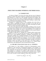
Figure 12.13 Iron loss density distribution (W/cm
3
)
a.) along circumpherential direction, b.) along radial direction, c.) along axial direction
(continued)

© 2002 by CRC Press LLC
Author: Ion Boldea, S.A.Nasar………… ………





c.)
Figure 12.13 (continued)
This way the radial or axial variation of losses (especially in the core) may

be obtained, provided that small enough temperature sensors are placed in key
locations. The winding average temperature is measured after turn-off by the
d.c. voltage/current method of stator winding resistance.

() ( ) ()






−+=
amb
C20
ss
TT
273
1
1RTR
0
(12.55)
Typical results are shown in Figure 12.13. [8] For the 4 pole IM in question,
the temperature variation along circumferential and axial directions in the back
core is small, but it is notable in the stator teeth. A notable decrease of loss
density with radial distance is present, as expected, (Figure 12.13c).
12.12. THERMAL ANALYSIS THROUGH FEM
In theory, the three-dimensional FEM alone could lead to a fully realistic
temperature distribution for a machine of any power and size, provided the
localization of heat sources and their levels are known.
The differential equation for heat flow is

()
t
T
cpTK
loss
∂
∂
γ=+∆∇
(12.56)
with K – local thermal conductivity (W/m
0
C); γ – local density (Kg/m
3
), p
loss
–
losses per unit volume (W/m
3
); and c – specific heat coefficient (J/
0
CKg). The
coefficients K, γ, c vary throughout the machine.
Two types of boundary conditions are usually present:
• Dirichlet conditions:
© 2002 by CRC Press LLC
Author: Ion Boldea, S.A.Nasar………… ………

()
*
bbb
Tt,z,y,xT =
(12.57)
The ambient temperature is such a boundary around the machine.
• Newman conditions:

0n
z
T
Kn
y
T
Kn
x
T
Kq
zzyyxx
=
∂
∂
−
∂
∂
−
∂
∂

−
(12.58)
n
x
, n
y
, n
z
are the x, y, z components of unit vector rectangular to the respective
boundary surface; q – the heat flow through the surface.
As a 3D FEM would require large amounts of computation time, 2D FEM
models have been built to study the temperature distribution either in the radial
cross section or in the axial cross section.
The radial cross section has a geometrical symmetry as seen in Figure
12.14.
77 C
0
82 C
0
85 C
0
127 C
0
126 C
0
95 C
0
a.) b.)
homogenous
equivalent

conductor layer
(slotless
computation
rotor)

Figure 12.14 Computation sector a.) and its restructuring to avoid motion influence b.)
To avoid the rotation influence on the modeling in the airgap zone, the rotor
sector is replaced by a motion-independent computation sector (Figure 12.14b).
[9]
After the temperature on the rotor surface is calculated and considered
“frozen,” the actual rotor sector is modeled.
It was found that the stator temperature varies radially and axially in a
visible manner, while the temperature gradient is much smaller in the rotor
(Figure 12.14a). [9] Similar results with 2D FEM are presented in Reference
[10].
3D FEM may be used for a more complete IM thermal modeling, treated
independently or together with the electromagnetic model for load (or speed)
transients; however the computation time becomes large.
Still, due to the dependence of thermal resistances and capacitors and loss
distribution on many “imponderable” factors, experimental methods (such as
advanced calorimetric ones) are needed to validate theoretical results, especially
when new machine configurations or design specifications are encountered.
© 2002 by CRC Press LLC