variable speed generatorsch (12)
Bạn đang xem bản rút gọn của tài liệu. Xem và tải ngay bản đầy đủ của tài liệu tại đây (3.2 MB, 43 trang )
© 2006 by Taylor & Francis Group, LLC
11-1
11
Transverse Flux and
Flux Reversal
Permanent Magnet
Generator Systems
11.1 Introduction 11-1
11.2 The Three-Phase Transverse Flux Machine (TFM):
Magnetic Circuit Design
11-6
The Phase Inductance L
s
• Phase Resistance and Slot Area
11.3 TFM — the d–q Model and Steady State 11-15
11.4 The Three-Phase Flux Reversal Permanent Magnet
Generator: Magnetic and Electric Circuit Design
11-18
Preliminary Geometry for 200 Nm at 128 rpm via Conceptual
Design • FEM Analysis of Pole-PM FRM at No Load • FEM
Analysis at Steady State on Load • FEM Computation of
Inductances • Inductances and the Circuit Model of
FRM • The d–q Model of FRM • Notes on Flux Reversal
Generator (FRG) Control
11.5 Summary 11-42
References
11-43
11.1 Introduction
There are certain applications, such as direct-driven wind generators, that have very low speeds (15 to
50 rpm) and microhydrogenerators with speeds in the range of up to 500 rpm and power up to a few
megawatts (MW) for which permanent magnet (PM) generators are strong candidates, provided the size
and the costs are reasonable.
Even for higher speed applications, but for lower power, today’s power electronics allow for acceptable
current waveforms up to 1 to 2.5 kHz fundamental frequency
f
1n
.
Increasing the number of PM poles 2
p
1
in the PM generator to fulfill the standard condition
(11.1)
thus becomes necessary.
Then, the question arises as to whether the PM synchronous generators (SGs) with distributed wind-
ings are the only solution for such applications, when the lowest pole pitch for which such windings can
be built is about
τ
min
≈ 30 mm, for three slots/pole. And, even at
τ
= 30 to 60 mm, is the slot aspect ratio
large enough to allow for a high enough electrical loading to provide for high torque density? The apparent
answer to this latter question is negative.
f p n n speed rps
nnn11
=⋅ −;()
© 2006 by Taylor & Francis Group, LLC
11-2 Variable Speed Generators
mind for pole pitches
τ
> 20 mm for large torque machines (hundreds of Newton meters [Nm]), but when
the pole pitch
τ
≈ 10 mm, they are again limited in electrical loading per pole, though there is about one
slot per pole (
N
s
≈ 2p
1
). In an effort to increase the torque density, the concept of a multipole span coil
winding can be used, which becomes practical, especially when the number of PM poles 2
p
1
> 10 to 12.
Two main breeds of PM machines were proposed for high numbers of pole applications: transverse
flux machines (TFMs) and flux reversal machines (FRMs).
The TFMs are basically single-phase configurations with single circumferential coil per phase in the
stator, embraced by U-shaped cores that create a variable reluctance structure with 2
p
1
poles. A 2p
1
pole
configurations placed along the shaft direction would make a two-phase or three-phase machine [1].
There are many other ways to embody the TFM, but the principle is the same. For example, the concept
can be extended by placing the PM pole structure in the stator, around the circumferential stator coil, while
the rotor is a passive variable reluctance structure with axial or radial airgap (Figure 11.2a and Figure 11.2b) [2].
The PM flux concentration is performed in the stator, in Figure 11.2 configurations, but the PM flux
paths in the rotor run both axially and radially; thus, the rotor has to be made of a composite magnetic
material (magnetic powder).
FIGURE 11.1 The single-sided transverse flux permanent magnet (PM) machine: (a) with surface PM pole rotor
and (b) with rotor PM flux concentration (interior PM poles).
FIGURE 11.2 Transverse flux machine (TFM) with stator permanent magnets (PMs): (a) with axial airgap and
(b) with radial airgap.
(a) (b)
Stator pole
Magnet
Winding
S
S
N
N
Rotor
Stator pole
(a)
(b)
Magnet
Winding
Rotor pole
Magnet
surface or an interior pole PM rotor is added (Figure 11.1a and Figure 11.1b). Two or three such
The nonoverlapping coil winding concept (detailed in Chapter 10) is the first candidate that comes to
© 2006 by Taylor & Francis Group, LLC
Transverse Flux and Flux Reversal Permanent Magnet Generator Systems 11-3
The TFMs with rotor or stator PM poles are characterized by the fact that the PM fluxes of all North
Poles add up at one time in the circumferential coil, and then, after the rotor travels one PM pole angle,
all South Poles add up their flux in the coil. Thus, the PM flux linkage in the coil reverses polarity 2
p
times per rotor revolution and produces an electromagnetic field (emf) E
s
:
(11.2)
where
l
stack
is the axial length of the U-shape core leg
θ
r
is the mechanical angle
B
g
is the PM airgap flux density
τ
is the pole pitch
Φ
PM
t
is the total flux per one turn coil
From Equation 11.2,
(11.2)
Equation (11.2) serves to prove that for the same coil and machine diameter (2
p
1
τ
= constant), the
number of turns, and stator core stack length, if the number
p
1
of U cores is increased, the emf is increased,
for a given speed. This effect may be called torque magnification [2], as torque
T
e
per phase (coil) is as
follows:
(11.3)
The structure of the magnetic circuit of the TFM is complex, as the PM flux paths are three-dimensional
either in the stator or in the rotor or in both.
Soft composite materials may be used for the scope, as their core losses are smaller than those in silicon
laminations for frequencies above 600 Hz, but their relative magnetic permeability is below 500
µ
0
at 1.0 T.
This reduces the magnetic anisotropy effect, which is so important in TFMs. This is why, so far, the
external rotor TFM with the U-shape and I-shape stator cores located in an aluminum hub is considered
the most manufacturable (Figure 11.3a and Figure 11.3b) [3]. Still, the additional eddy current losses in
the aluminum hub carrier are notable.
Figure 11.4b) to increase the torque per PM volume ratio, they prove to be difficult to manufacture.
While increasing the torque/volume and decreasing the losses per torque are key design factors, the
power factor of the machine is essential, as it defines the kilovoltampere of the converter associated with
the TFM for motoring and generating.
FIGURE 11.3 The three-phase external permanent magnet (PM)-rotor transverse flux machine (TFM): (a) internal
stator and (b) external rotor.
EWp
d
dt
Bpl
s
PM
t
r
r
PM
t
r
gstack
=− ⋅ ⋅
∂
∂
⋅
∂
∂
≈
11
φ
θ
θ
φ
θ
; ⋅⋅ ⋅
τθ
sin p
r
EWpBl nWBpl
s g stack g st
≈− ⋅ ⋅ ⋅ ⋅ ⋅ ⋅ =− ⋅ ⋅ ⋅ ⋅
11
2
11
2
τπ τ
aack r
p⋅⋅
ωθ
1
sin
T
EI
n
np
e
sr r
phase
=
⋅
⋅⋅
=⋅⋅⋅
() ()
;
θθ
π
ωπ
1
11
2
2
(a) (b)
Though double-sided TFMs with rotor PM flux concentration were proposed (Figure 11.4a and
© 2006 by Taylor & Francis Group, LLC
11-4 Variable Speed Generators
The ideal power factor angle
ϕ
1
of the TFM (or of any PM synchronous machine [SM]) may be defined,
in general, as follows:
(11.4)
where
L
s
is the synchronous inductance of the machine
I
s
is the phase current
Equation 11.4 is valid for a nonsalient pole machine behavior (surface PM pole machines).
For the interior PM pole TFM with flux concentration and a diode rectifier, the machine is forced to
operate at about unity power factor. In such conditions, what is the importance of
ϕ
1n
as defined in
Equation 11.4? It is to show the power factor angle of the machine for peak torque (pure
I
q
current
control for the nonsalient pole machine). For generality, the presence of a front-end pulse-width mod-
ulated (PWM) converter is necessary to extract the maximum power and experience the
ϕ
1n
power factor
angle conditions. The power factor at rated current cos
ϕ
1n
is a crucial performance index.
In any case, the larger the machine inductance voltage drop per emf, the lower the power factor
goodness of the machine. From this point of view, the PM flux concentration, though it leads to larger
torque/volume, also means a higher inductance, inevitably. The claw-pole stator cores were proposed to
improve the torque/volume, but the result is still modest [3], due to low power factor. Consequently,
only at the same torque density as in the surface PM pole machine, can the TFM with PM flux concen-
tration eventually produce the same power factor at better efficiency and with a better PM usage. While
the above rationale in power factor is valid for all PM generators, the problem of manufacturability
remains heavy with TFMs.
In order to produce a more manufacturable machine, the three-phase flux reversal PM machine (FRM)
was introduced [4]. FRM stems from the single-phase flux-switch generator [5] and is basically a doubly
salient stator PM machine. The three-phase FRM uses a standard silicon laminated core with 6
k large
semiclosed slots that hold 6
k nonoverlapping coils for the three phases.
Within each stator coil large pole, there are 2
n
p
PM poles of alternate polarity. Each such PM pole
spans
τ
PM
. The large slot opening in the stator spans 2/3
τ
PM
. The rotor has a passive salient-pole laminated
core with
N
r
poles. To produce a symmetric, basically synchronous, machine,
(11.5)
FIGURE 11.4 Double-sided transverse flux machine (TFM) (a) without and (b) with rotor permanent magnet (PM)
flux concentration.
(a) (b)
ϕ
ω
ω
1
1
1
1
n
ssn
s
LI
E
=
⋅⋅
−
tan
()
2266
2
3
⋅⋅ =⋅⋅⋅+⋅⋅
⋅Nnkk
rPM p PM
ττ
© 2006 by Taylor & Francis Group, LLC
Transverse Flux and Flux Reversal Permanent Magnet Generator Systems 11-5
where
k = 1, 2, …
n
p
= 1, 2, …
A typical three-phase FRM is shown in Figure 11.5a and Figure 11.5b.
As for the TFM, the PM flux linkage in the phase coils changes polarity (reverses sign) when the rotor
moves along a PM pole span angle. The structure is fully manufacturable, as it “borrows” the magnetic
circuit of a switched reluctance machine. However, the problem is, as for the TFM, that the PM flux
fringing reduces the ideal PM flux linkage in the coils to around 30 to 60%, in general. The smaller the
pole pitch
τ
PM
, the larger the fringing and, thus, the smaller the output. There seems to be an optimum
thickness of the PM
h
PM
to pole pitch
τ
PM
ratio, for minimum fringing.
On the other hand, the machine inductance
L
s
tends to be reasonably small, as end connections are
reasonable (nonoverlapping coils) and the surface PM poles secure a notably large magnetic airgap.
Still, in Reference 4, for a 700 Nm peak torque at 7 N/cm
2
force density, the power factor would be
around 0.3. In order to increase the torque density for reasonable power factor, PM flux concentration
FIGURE 11.5 Three-phase flux reversal machine (FRM) with (a) stator surface permanent magnets (PMs)
(
N
s
= 12; n
p
= 2; N
r
= 28) and (b) inset PMs (N
s
= 12; n
p
= 3; N
r
= 40).
FIGURE 11.6 Three-phase flux reversal machine (FRM) with stator permanent magnet (PM) flux concentration.
(a) (b)
PM
Air
Winding
Rotor
may be performed in the stator (Figure 11.6) or in the rotor (Figure 11.7).
© 2006 by Taylor & Francis Group, LLC
11-6 Variable Speed Generators
The FRM with stator PM flux concentration is highly manufacturable, but as the pole pitch
τ
PM
gets
smaller, because the coil slot width
w
s
is less than
τ
PM
, the power factor tends to be smaller. For
τ
PM
= 10
mm and
w
s
=
τ
PM
and a 4w
s
height, with j
peak
= 10 A/mm
2
and slot filling factor k
fill
= 0.4, the slot
magnetomotive force (mmf) W
c
I
peak
is as follows:
Larger slot mmfs could be provided for the TFM and FRM with stator surface PM poles. However,
the configuration in Figure 11.7 allows for the highest PM flux concentration, which may compensate
for the lower W
c
I
peak
and allow for lower-cost PMs, because the radial PM height is generally larger than
3 to 4
τ
PM
. As with any PM flux concentration scheme, the machine inductance remains large. But, for
not so large a number of poles, the machine’s easy manufacturability may pay off. On the other hand,
the FRM with rotor PM flux concentration configuration (Figure 11.7) provides for large torque density,
because, additionally, the allowable peak coil mmf may be notably larger than that for the configurations
The rotor mechanical rigidity appears, however, to be lower, and the dual stator makes manufacturability
a bit more difficult. Still, conventional stamped laminations can be used for both stator and rotor cores.
To provide more generality to the analysis that follows, we will consider only the three-phase TFMs
and FRMs, which may work both as generators and motors with standard PWM converters and position-
triggered control.
11.2 The Three-Phase Transverse Flux Machine (TFM): Magnetic
Circuit Design
external rotor. The iron behind the PMs on the rotor may be, in principle, solid iron, which is a great
advantage when building the rotor.
FIGURE 11.7 Three-phase flux reversal machine (FRM) with rotor permanent magnet (PM) flux concentration
and dual stator.
Rotor
Shaft
SS
SS
SS
SS
S
S
SS
SS
SS
SS
SS
SS
SS
SS
SS
SS
SS
SS
SS
SS
SS
SS
Stator
Winding
Secondary
stator
NN
NN
NN
NN
NN
SS
SS
NN
NN
NN
NN
NN
NN
NN
NN
NN
NN
NN
NN
NN
NN
NN
NN
NN
NN
WI wmm wmmk j
c peak s s fill peak
⋅= ⋅⋅ ⋅⋅=⋅⋅[] []4104100 0 4 10 1600⋅⋅=./Aturns slot
with stator PM flux concentration (Figure 11.6).
The configuration for one phase may be reduced to the one in Figure 11.1a, but inverted, to have an
© 2006 by Taylor & Francis Group, LLC
Transverse Flux and Flux Reversal Permanent Magnet Generator Systems 11-7
carriers that hold tight the stator I- and U-cores are the main new frame elements that have to be
fabricated by precision casting.
have been implanted in the aluminum carrier. Then, the I-cores are placed one by one in their locations
It was shown that, in order to reduce the cogging torque, the stator U- and I-cores of the three phases
have to be shifted by 120 electrical degrees with respect to each other [6]. In such a case, the three phases
are magnetically independent, though the PMs are axially aligned on the rotor for all three phases.
mensional in the stator. However, as the flux paths are basically radial in the PMs and circumferential-radial
in the rotor back iron, the rotor back iron may be made of mild solid steel. The bidimensional flux paths
in the stator allow for the use of transformer laminations in the U- and I-cores.
There is, however, substantial PM flux fringing, which crosses the airgap and closes the path between
the stator U- and I-cores in the circumferential direction. To reduce it, both U- and I-cores should expand
circumferentially less than a PM pole pitch
τ
PM
: b
u
, b
i
<
τ
PM
. Also, to reduce axial PM flux fringing, the
axial distance between the U-core legs l
slot
should be equal to or larger than the magnetic airgap (l
slot
> g +
h
PM
). But, l
slot
is, in fact, equal to the width of the open slot where the stator coil is placed.
The U-core yoke h
yu
and the I-core h
yi
heights should be about equal to each other and around the
value of 2/3 l
stack
in order to secure uniform and mild magnetic saturation in the stator iron cores. Also,
the rotor yoke radial thickness h
yr
should be around half the PM pole pitch, as half of the PM flux goes
We will now approach performance through an analytical method, accounting approximately for
magnetic saturation in the stator and iron cores.
Each PM equivalent mmf F
PM
= H
c
h
PM
(H
c
is the coercive field of the PM material) “is responsible”
for one magnetic airgap h
gM
= g + h
PM
. This way, the equivalent magnetic circuit on no load (zero current)
is as in Figure 11.9:
(11.6)
FIGURE 11.8 Transverse flux machine (TFM) — aluminum carrier with interior stator cores and coil.
Armature
winding
Aluminum
carrier
U-shaped
core
I-shaped
core
R
hg
bl b b
PM g
PM
PM stack PM u
+
=
+
⋅⋅⋅ +
µ
0
2()/
Also, the stator U-shape and I-cores (Figure 11.4a) may be made of silicon laminations. The aluminum
through the rotor magnetic yoke (Figure 11.9).
on top of the coil (Figure 11.8).
Apparently, the circumferential coil has to be wound turn by turn on a machine tool after the U-cores
As seen in Figure 11.3a, the PM flux paths are basically three-dimensional in the rotor but only bidi-
© 2006 by Taylor & Francis Group, LLC
11-8 Variable Speed Generators
where
R
PM+g
is the PM and airgap magnetic reluctance
b
PM
is the PM width (b
PM
/τ
PM
= 0.66 to 1.0)
b
u
is the U-core width
R
fringe
is the magnetic reluctance of the PM fringing flux between the stator U- and I-cores through
the airgap, corresponding to one leg of the U- and I-cores.
To a first approximation,
(11.7)
Straight-line magnetic flux paths are considered between U- and I-cores up to the height of the I-core
fringe
. The stator U- and I-core
reluctances R
yu
and R
yi
are as follows:
(11.8)
(11.9)
Also,
(11.10)
where µ
cu
, µ
yu
, µ
yi
, and µ
yr
are the magnetic permeabilities dependent on magnetic saturation. As the PM
equivalent mmf F
c
is given, once all the PM geometry and material properties are known, an iterative
procedure is required to solve the magnetic circuit in Figure 11.9. To start with, initial values are given
to the four permeabilities in the iron parts: µ
cu
(0), µ
yu
(0), µ
yi
(0), and µ
yr
(0). With these values, the flux
in the stator and rotor core parts and Φ
PMax
are computed.
FIGURE 11.9 The magnetic equivalent circuit for permanent magnets (PMs) in the position for maximum flux in
the stator coil.
R
PM+g
2 R
yr
F
PMax
F
PMax
R
PM+g
R
PM+g
R
PM+g
R
yi
+ R
yu
R
fringe
R
fringe
F
PM
F
PM
F
PM
F
PM
R
h
b
fringe
PM
b
PM yu
h
PM yi
≈
⋅
+
−
⋅
⋅
µ
τ
µ
0
2
0
2
1
ll
bb
stack
yu yi
; =
R
hh
bl
ll
yu
slot yi
cu u stack
stack slot
=
⋅+
⋅⋅
+
+
2( )
µ µµ
yu yu u
hb⋅⋅
R
l
hb
l
hb
b
yi
slot
yi yi i
stack
yi yi i
i
≈
⋅⋅
+
⋅
⋅⋅
≈
µµ
4
; bb
u
R
bl
yr
PM
yr yr stack
=
⋅⋅
τ
µ
(Figure 11.8). The axial fringing may be added as a reluctance in parallel to R
© 2006 by Taylor & Francis Group, LLC
Transverse Flux and Flux Reversal Permanent Magnet Generator Systems 11-9
But, the average flux densities in various core parts are straightforward, once Φ
PMax
is known:
(11.11)
Once the average values of flux densities B
cu
, B
yu
, B
yi
, and B
yr
are computed, and from the magnetization
curve of the core materials, new values of permeabilities µ
cu
(1), µ
yu
(1), µ
yi
(1), and µ
yr
(1) are calculated.
The computation process is reinitiated with renewed permeabilities:
(11.12)
such as to speed up convergence.
The computation is ended when the largest relative permeability error between two successive com-
putation cycles is smaller than a given value (say, 0.01). This way, the maximum value of the PM flux
per pole (U-core), Φ
PMax
, in the coil, is obtained.
The PM flux per pole varies from +Φ
PMax
to −Φ
PMax
when the rotor moves along a PM pole angle
(2
π
/2p
1
mechanical radians). What is difficult to find out analytically, even with a complicated magnetic
circuit model with rotor position permeances, is the variation of Φ
PM
with rotor position from +Φ
PMax
to −Φ
PMax
and back.
It was shown by three-dimensional (3D) finite element method (FEM) that the PM flux per pole varies
trapezoidally with rotor position (Figure 11.10).
We may consider, approximately, that the electrical angle
θ
econst
, along which the PM flux stays constant
(Figure 11.10) is rather small and is as follows [3]:
[rad] (11.13)
Magnetic saturation alters not only Φ
PMax
but also the value of
θ
econst
, tending to flatten the trapezoidal
waveform and bringing it closer to a rectangular waveform of lower height. But, local magnetic saturation
plays an even more important role when the machine is under load.
FIGURE 11.10 Permanent magnet (PM) flux per stator pole vs. rotor position.
φ
PMax yu stack cu yu yu yu yi i yi
bl B bhB hbB=⋅ ⋅=⋅⋅=⋅⋅
φφ
PMax
yr yr stack
Bhl
2
=⋅⋅
µµ µµ
( ) ( ) ( ( ) ( )); . .1 0 1 0 02 03=+ − =−
iii
cc
θ
τ
π
econst
PM u
PM
bb
≈−
+
⋅
⋅
1
24
(
)
q
er
= p
1
q
r
-F
PMax
F
PMax
F
PM
(q
er
)
2p
p
p =q
const
1
−
2
(b
PM
+ b
u
)
4t
PM
© 2006 by Taylor & Francis Group, LLC
11-10 Variable Speed Generators
In general, the computation of the force density (in N/cm
2
) on the rotor surface is done via the Maxwell
stress tensor through FEM. The magnetic saturation presence is evident when the force is calculated for
various rotor positions for constant phase current (Figure 11.11).
The PM flux per pole and the emf, obtained through 3D FEM, look as shown in Figure 11.12.
The instantaneous emf per phase E is as follows (Equation 11.2 and Equation 11.3):
(11.14)
(11.15)
So, the emf per phase has a waveform in time, which emulates the waveform of dΦ
PM
(
θ
er
)/d
θ
er
. The above
derivative maximum decreases when the PM pole pitch decreases due to the increase in fringing flux,
FIGURE 11.11 Typical force density (N/cm
2
) vs. rotor position and various constant current values.
FIGURE 11.12 Typical finite element method (FEM)-extracted permanent magnet (PM) flux and its derivative vs.
rotor position.
6
4
2
0
I = 0
I
rated
I
peak
−2
q
er
p
p
2
f
t
N
cm
2
EWp
d
d
np
PM er
er
=⋅⋅ ⋅⋅⋅⋅
1
2
φθ
θ
π
()
θω
er r
t=⋅
10
−4
−10
−4
0
90° 180°
dF
PM
/dq
er
F
PM
(Wb)
© 2006 by Taylor & Francis Group, LLC
Transverse Flux and Flux Reversal Permanent Magnet Generator Systems 11-11
when the number of poles increases. Consequently, there should be an optimum number of PM poles
for a given rotor diameter that produces maximum emf for given W
1
, stack length, and mechanical gap g.
If the phase emf is considered through its fundamental, the average torque per phase, when the emf
and current are phase shifted by angle
γ
1
, is as follows:
(11.16)
where I
1
is the root mean squared (RMS) phase current, and
(11.17)
11.2.1 The Phase Inductance L
s
The phase inductance L
s
is composed from the leakage inductance L
sl
and the main path inductance L
m
.
As the magnetic circuits of the three phases are separated, there is no coupling inductance between phases.
L
s
refers to one phase only. The airgap inductance L
m
is, approximately,
(11.18)
where k
s
is an equivalent magnetic saturation coefficient that considers the contribution of the iron parts
to the total mmf along a flux path. k
f
is a fringing coefficient that takes care of the fringing flux in the
airgap: k
f
< 0.2 in general.
In a similar manner, we may treat the maximum flux per pole:
(11.19)
k
fringe
is the PM fringing flux coefficient (very different from k
f
) that can go as high as two (k
fringe
= 0.7
to 2), while k
s
is the magnetic saturation coefficient. In general, k
s
has to be calculated when current is
present in stator phases. The leakage inductance may be calculated approximately from slot leakage flux,
extended between U-cores, because I-cores “create” a moderate “slot leakage effect”:
(11.20)
k
i
accounts for the leakage inductance between the U-cores. In general, k
i
< 0.2 to 0.3.
As the total iron area, as seen along the airgap, by the stator coil, is independent of the number of
poles, both L
m
and L
sl
are independent of the number of poles 2p
1
. At the same time, the emf E and the
torque (T
e
)
aphase
per phase are proportional to the number of poles if the increasing fringing (k
fringe
) with
the number of poles is not considered.
11.2.2 Phase Resistance and Slot Area
The phase resistance R
s
is straightforward:
(11.21)
The ampereturns per phase (RMS value), W
1
I
1
, may be calculated from Equation 11.16 once the torque
per phase requirement is given.
()
cos cos
T
EI
n
Wp I
eaph
sPMax
=
⋅⋅
⋅⋅
=
⋅⋅ ⋅⋅
111
2
1
2
γ
π
φ γγ
1
2
φθ φ θ
PM r PMax r
p() cos( )=⋅⋅
L
W
R
Wp l
gh
m
mag
bb
stack
uPM
=⋅ ≈⋅
⋅⋅ ⋅
⋅+
+
µµ
0
1
2
0
1
2
2
4(
PPM s f
kk)( )( )⋅+ ⋅+11
φ
PMax gi
PM u
stack
sfringe
B
bb
l
kk
=⋅
+
⋅⋅
++2
1
11()( )
LW
h
l
pb k
sl
s
slot
ui
≈⋅ ⋅
⋅
⋅⋅ ⋅+
µ
01
2
3
1()
R
DhhW
s
is yi s
copper
WI
j
con
≈
⋅+⋅+⋅
⋅
⋅
π
σ
()2
1
2
11
© 2006 by Taylor & Francis Group, LLC
11-12 Variable Speed Generators
The rated (continuous) current density j
con
depends on the machine duty cycle, type of cooling, and
design optimization criterion (maximum efficiency or minimum machine cost, etc.). In general, j
con
= 4
to 12 A/mm
2
. The window area in the slot A
slot
is as follows:
(11.22)
The total slot filling factor k
fill
is, in general, k
fill
= 0.4 to 0.6. The larger values correspond to the preformed
coils eventually made of rectangular cross-sectional conductors.
Example 11.1
Consider sizing a three-phase TFM generator with surface PM interior rotor and single-sided stator
(with U- and I-cores) that has the following specifications: T
en
= 200 kNm and n
n
= 30 rpm.
Solution
While part of the design formulas are included in the previous paragraphs, some new ones are
introduced here. They are mainly related to the stator bore diameter D
is
with given l
stack
/D
is
ratio (
λ
= l
stack
/D
is
= 0.05 to 0.1).
We make use of the force density f
t
= 2 to 8 N/cm
2
to determine the interior stator diameter D
is
:
(11.23)
In our case, with
λ
= 0.05, f
t
= 2.66 N/cm
2
:
(11.24)
The stack length is as follows:
l
stack
=
λ
D
is
= 0.05·2.515 = 0.1257 m (11.25)
We now have to choose the airgap g, first.
For such a large diameter, an airgap of 1.5 to 5 mm is required for mechanical rigidity reasons. Let
us consider g = 4·10
−3
m. The ideal airgap flux density B
gi
produced by the PM magnets in the airgap
is as follows:
(11.26)
with B
r
= 1.3 T, µ
rem
= 1.04 µ
rem
at 100°C (very good NeFeB magnets: B
r0
= 1.37 T at 20°C).
We need to choose a large PM height h
PM
, because the actual airgap flux density will be notably
reduced by the fringing (k
fringe
≈ 2). So, h
PM
= g = 3 · 4 · 10
−3
= 12 · 10
−3
= 1.2 · 10
−2
m. Consequently,
from Equation 11.26,
(11.27)
Now the maximum flux per pole may be calculated if we adopt the number of poles 2p
1
.
Ahl
WI
jk
slot s slot
con fill
=⋅ =
⋅
⋅
11
D
T
f
T
D
fD l
is
e
t
e
is
tis stac
=
⋅⋅⋅
=⋅⋅⋅⋅⋅⋅
32
32
3
πλ
π
;
kk
Dm
is
=
⋅⋅ ⋅ ⋅
=
200000
300526610
2 525
4
3
π
.
BB
h
hg
gi r
PM
PM
=⋅
+
BT
gi
=
⋅
+
=
13 12
12 4
0 975
.
.
© 2006 by Taylor & Francis Group, LLC
Transverse Flux and Flux Reversal Permanent Magnet Generator Systems 11-13
In general, the PM pole pitch
τ
PM
should be higher than the total (magnetic) airgap: g + h
PM
=
1.6 · 10
−2
m. The number of poles 2p
1
is, thus,
(11.28)
Let us consider 2p = 400 poles and
τ
PM
= 1.974 · 10
−2
m. The fundamental frequency at 30 rpm is
f
n
= p
1
· n
n
= 200 · 30 / 60 = 100 Hz, which is a reasonable value in terms of core losses. Now,
the maximum PM flux per pole from Equation 11.19, with k
fringe
= 2.33; k
s
= 0.1; b
PM
/
τ
PM
= 0.85;
b
u
/
τ
PM
= 0.8 is as follows:
(11.29)
We now turn directly to the torque expression to find the ampere turns per phase W
1
I
1
(RMS value)
from Equation 11.16, with
γ
1
= 0 (emf and current in phase):
(11.30)
This is a reasonable value.
The slot area required for the coil for j = 6 A/mm
2
and k
fill
= 0.6, from Equation 11.22, is as follows:
(11.31)
Taking
l
slot
= 2(g + h
PM
) = 32 mm (11.32)
the slot height h
s
is
(11.33)
The fact that h
s
/l
slot
≈ 1 will lead to a smaller leakage inductance, which is favorable for a good power
factor.
Consider h
yi
= h
yu
= 2/3 · l
stack
= 0.083 m. Then, from Equation 11.21, the stator phase resistance R
s
is
(11.34)
The total winding losses for the machine, P
con
, are as follows:
(11.35)
2
2 515
002
394 8⋅=
⋅
=
⋅
=p
D
is
PM
π
τ
π
.
.
.
φ
PMax gi
PM u
stack
fringe s
B
bb
l
kk
=⋅
+
⋅⋅
+⋅+2
1
11()(
))
.
(.)(.
=⋅⋅⋅ ⋅
+⋅+
−
0 975 1 628 10
0 2515
2
1
123310
2
11
0 5986 10
3
)
.=⋅
−
Wb
WI
T
p
en
PMax
11
2
3
2
2
3
200 10 2
3 200 0 598
⋅=
⋅
⋅⋅
=
⋅⋅
⋅⋅
φ
. 6610
3885
3
⋅
=
−
Aturns
A
WI
jk
mm
slot
con fill
=
⋅
⋅
=
⋅
=
11
2
3885
606
1079 16
.
.
h
A
l
mm
s
slot
slot
== =
1079
32
33 72.
R
s
=
⋅⋅⋅ +⋅ +
−
⋅
2 3 10 2 515 2 0 083 0 03372
8
3885
6
.( )
π
110
1
23
1
2
6
0 3026 10⋅= ⋅⋅
−
WW.
PRI kW
con s
=⋅ ⋅ =⋅ ⋅ ⋅ =
−
3 3 0 3206 10 3885 13 70
1
232
© 2006 by Taylor & Francis Group, LLC
11-14 Variable Speed Generators
The electromagnetic power, P
elm
, is
(11.36)
The winding losses are about 2% of input power.
Now we need to calculate the synchronous inductance L
s
= L
m
+ L
sl
. From Equation 11.19,
(11.37)
Also, from Equation 11.20, L
se
, the leakage inductance is as follows:
(11.38)
So,
(11.39)
The emf E (rms value) is as follows:
(11.40)
The ideal power factor angle
ϕ
1
(for γ = 0) is
(11.41)
The very good value of the power factor angle for E and I in phase is a clear indication of machine
volume reduction reserve (the specific tangential force is only 2.66 N/cm
2
).
11.3 TFM — the d–q Model and Steady State
Let us consider here that TFM is provided with a surface PM rotor, and thus, the synchronous inductance
L
s
is independent of rotor position. We adopt this configuration, as the power factor may be higher due
to smaller inductance L
s
, even though at slightly smaller torque density than for the PM flux concentration
configurations. Though the emf waveform is not quite sinusoidal, we consider it here as sinusoidal.
PT n
elm e n
=⋅⋅⋅= ⋅ ⋅⋅⋅ =2 200 10 2
30
60
628
3
ππ
kW
L
Wp l
gh k
m
bb
stack
PM s
uPM
=
⋅⋅⋅ ⋅
⋅+ ⋅+ ⋅
+
µ
01
2
2
41()()(()
.
1
1 256 10 200 1 62 10
41
62
0 2515
2
+
=
⋅⋅⋅⋅⋅
⋅
−−
k
f
( . ) ( . )
.
610 1 01 1 01
1 321 10
2
2
1
2
5
1
⋅⋅+⋅+
⋅=
⋅
⋅
−
−
WW
22
[]H
LW
h
l
kpb
sl
s
slot
iu
=⋅ ⋅
⋅
⋅+ ⋅ ⋅
=⋅
−
µ
01
2
1
3
1
1 256 10
()
.
66
1
2
0 03372
3 0 032
1 0 3 200 0 016 1 8⋅
⋅
⋅+ ⋅ ⋅ ⋅ =
.
.
(.) . .W 334 10
6
1
2
⋅⋅
−
W
LLL W
sl m se
=+=
⋅
+⋅
⋅
−
−
1 321 10
2
1 834 10
5
6
1
2
.
. ==⋅⋅
−
0 844 10
5
1
2
. W
E
Tn
III
en
=
⋅⋅⋅
⋅⋅
=
⋅
⋅
=
⋅
2
3
628 10
3
209 3 10
1
3
1
3
π
γ
cos
.
11
ϕ
ω
π
1
1
11
1
5
2 100 0 844 10
2
n
s
LI
E
=
⋅⋅
=
⋅⋅ ⋅ ⋅
−−
−
tan tan
.
008 33 10
2 544 10 3
3
1
2
1
2
18
.
tan ( .
⋅
⋅⋅
=⋅⋅
−−
WI
8885 0 384 21 0 933
21
1
)tan . ;cos .==°=
−
ϕ
n
The data of the preliminary design are given in Table 11.1.
© 2006 by Taylor & Francis Group, LLC
Transverse Flux and Flux Reversal Permanent Magnet Generator Systems 11-15
The d–q model is thus straightforward, if the core losses are neglected for the time being:
(11.42)
where
W
1
is the turns per coil (phase)
p
1
is the pole pairs:
For steady state
Figure 11.13b for pure I
q
control (I
d
= 0) and for unity power factor (with diode rectifier). Pure I
q
control for L
s
= constant corresponds to maximum torque per current, but the machine requires
reactive power for magnetization. A controlled front rectifier is required.
The performance is acceptable, but the force density is not large enough.
For the diode rectifier, the current always contains an I
d
component (Figure 11.13b), and thus, the
torque is produced with more losses. However, the reactive power required is zero, and the diode rectifier
is less expensive. If constant direct current (DC) link voltage operation at variable speed is required,
either an active front or PWM converter is provided on the machine side or a diode rectifier plus a
TABLE 11.1 Example Design Summary
Electromagnetic torque T
e
= 200 kNm
Speed n
n
= 30 rpm
Force density f
t
= 2.66 N/cm
2
Current density j
con
= 9 A/mm
2
Stator interior diameter D
is
= 2.515 m
Stator stack U-core leg l
stack
= 0.1257 m
Mechanical gap g = 4·10
−3
m
Permanent magnet radial thickness h
PM
= 12·10
−3
m
Number of permanent magnet poles 2·p = 400
Fundamental frequency f
n
= 100 Hz
Permanent magnet pole pitch
τ
PM
= 1.974·10
−2
m
Axial room between U-core legs l
slot
= 32·10
−3
m
U-core width b
u
/τ
PM
= 0.8
Permanent magnet width per pole b
PM
/τ
PM
= 0.85
U-core yoke height h
yu
= 2/3·l
stack
I-core yoke height h
yi
= h
yu
Slot useful height h
s
= 33.72·10
−3
m
Total U-core interior height h
s
+ h
yi
External stator diameter D
os
= 2.621 m
Total axial length per phase l
slot
+ 2·l
stack
= 0.032 + 0.2515 m = 0.2835 m
Total axial length for three phases l
axial
= 3·(l
slot
+ 2·l
stack
) = 0.85 m
Reduction of permanent magnet flux due to fringing 1/(1 + k
fringe
) = 1/3
Stator resistance per phase R
s
= 0.454·10
−3
·W
1
2
Stator inductance per phase L
s
= 0.844·10
−5
·W
1
2
Emf at f
1
= 100 Hz E = 53.61·W
1
(rms)
Stator copper losses P
con
= 20.55 kW
Electromagnetic power T
e
·2·
π
·n
n
= 628 kW
Power factor angle
(with E and I in phase)
ϕ
1n
≈ 21°; cos
ϕ
n
= 0.933
IR V
d
dt
j
jL
s
s
s
s
rs
sd qdPMs
⋅+ =− −⋅⋅
=+⋅ = +
ψ
ωψ
ψψ ψψψ
; ⋅⋅ = ⋅
=+⋅ =+⋅ =
ILI
IIjIVVjV
dq sq
s
dq
s
d q PM PMa
;
;;
ψ
ψφ
xx
Wp⋅⋅
11
Tp I I p I
edqqdPMq
=⋅⋅ ⋅− ⋅ =⋅⋅ ⋅
3
2
3
2
11
()
ψψ ψ
d
dt
= 0, and the vector diagram for generating is as shown in Figure 11.13a and
© 2006 by Taylor & Francis Group, LLC
11-16 Variable Speed Generators
DC–DC boost converter is required. The core losses might be considered, mainly for steady state, as
follows:
(11.43)
In Equation 11.43, the core losses are considered to be produced by the resultant flux in the machine,
in the presence of stator current. The core losses p
iron
might be determined from tests that segregate the
The efficiency may be defined as follows:
(11.44)
The rotor losses p
rotor
refer to the eddy current losses in the PMs, which may be neglected only for
f
1
≤ 100 Hz, in general. The strayload losses are included in p
iron
and p
copper
, but the eddy current losses in
the aluminum carriers of the U- and I-cores are individualized as p
Al
and may be calculated only through
3D FEM eddy current models [7].
When the fundamental frequency goes up, above 100 Hz, p
iron
and p
rotor
become important and have
Example 11.2
Consider the TFM design in Example 11.1, and calculate the number of turns per phase for a line
voltage V
Ln
= 584 V (RMS) — star connection — at rated speed for E, I in phase, and for the same
number of turns W
1
and unity power factor, and calculate the performance for the same current as above.
Solution
We simply make use of the vector diagram (Figure 11.13a), where y
PM
is
(11.45)
FIGURE 11.13 The transverse flux machine (TFM) vector diagram for steady state: (a) pure I
q
control and (b) with
power factor control (with diode rectifier).
d
δ
V
= ϕ
1
< 0
δ
V
jq
i
s
= jI
q
ω
r
LsjI
q
L
s
I
d
L
s
jI
q
jI
q
Ψ
PM
d
jq
ω
r
Ψ
PM
−jω
r
Ψ
s
Ψ
s
−jω
r
L
s
I
s
−jω
r
Ψ
s
−jω
r
L
s
I
s
V
s
−R
s
I
s
V
s
−R
s
I
s
E
s
I
d
E
s
I
s
(a) (b)
p
R
iron
rs
iron
=⋅
⋅
3
2
2
ωψ
η
=
+++ + +
P
Pppp p p
el
el mec iron copper rotor Al
2
2
ψ
ωπ
PM
r
Erms
W
W
V
=
⋅
=
⋅⋅
⋅⋅
=⋅
()
.
.
2
53 61 2
2 100
0 1203
1
1
ssn
Ln
Vrms
V=
⋅
=
⋅
=
()2
3
584 2
3
476
to be dealt with using great care (see Chapter 10 for more details).
iron losses, or they may be calculated from analytical or FEM models, as shown in Chapter 10.
© 2006 by Taylor & Francis Group, LLC
Transverse Flux and Flux Reversal Permanent Magnet Generator Systems 11-17
(11.46)
or
(11.47)
With W
1
I
1
= 3885 Aturns/coil, we obtain W
1
≈ 6 turns/coil. As the core and mechanical losses have
not been considered, the efficiency will reflect only the presence of the already calculated copper losses:
(11.48)
Alternatively,
(11.49)
with
(11.50)
(11.51)
The difference in efficiency from the two formulas above is only due to calculation errors, as the
model is the same.
Now, for the second case, we have to notice that if we consider the same phase current (RMS) I
1
and voltage V
Ln
, the vector diagram in Figure 11.13b provides the following:
(11.52)
with W
1
= 6 turns, I
1
= 647.5 A, we can calculate, from Equation 11.52, the terminal voltage:
(11.53)
(11.54)
The line terminal voltage for the same current decreased notably for unity power factor.
Now, the output power is only
(11.55)
EErms V RI
ssss
=⋅=⋅+⋅() cos2
1
ϕ
75 59 476 0 933 0 454 10 2
1
3
1
2
1
⋅= ⋅ + ⋅ ⋅⋅⋅
−
WWI
η
=
−
==
−
=
Pp
P
P
P
elm con
elm elm
1
1
2
1
628 13 70
628
614
.
.
33
628
0 978
kW
kW
= .
η
ϕ
en
Ln
elm
VI
P
=
⋅⋅⋅3
11
1
cos
I
WI
W
A
1
11
1
3885
6
647 5=
⋅
==.
η
en
=
⋅⋅⋅
⋅
==
3 584 647 0 933
628 10
609
628
0 971
3
.
.
()VRI LI E
ss s s
+⋅ + ⋅⋅=
1
2
1
22
1
22
ω
′
=−⋅⋅−⋅
=⋅−⋅⋅
VE LIRI
ss ssss
2
1
222
2
75 59 6 2 1
ω
π
(. ) ( 000 1 5044 10 6 647 5
0 3026 10
52 4 2
3
1
2
⋅⋅⋅⋅
−⋅⋅
−
−
.).
. W
⋅⋅ ⋅ = − =IV
1
2 396 48 9 945 386 63 .
′
=
′
⋅
=⋅= <V
V
VV
L
s
3
2
386 63
3
2
473 40 584
() . . .
cos
′
=⋅ ⋅ =
=
PkW
21
1
3 473 40 647 5 530 29
ϕ
From Figure 11.13a,
© 2006 by Taylor & Francis Group, LLC
11-18 Variable Speed Generators
So, for the same number of turns W
1
= 6 and the same conductor cross-section and current and speed,
with a diode rectifier, the generator will produce 20% less power. The additional reactive power provided
through the active front PWM converter, when E and I are in phase, allows for delivering power in better
conditions (higher voltage and power).
Note on the Control of TFM
Once a three-phase machine is considered, the control may be implemented with sinusoidal current (for
almost sinusoidal emf) or with trapezoidal current (for trapezoidal emf), with third harmonic tapping,
if a diode rectifier is used. The control system, with or without motion sensors, is practically the same
control.
The methods used to reduce the cogging torque are similar to those for standard PMSGs.
It is to be seen if the TFM will make it to the markets soon, at least as a low-speed high-torque direct-
driven generator.
11.4 The Three-Phase Flux Reversal Permanent Magnet
Generator: Magnetic and Electric Circuit Design
As mentioned in the section on TFMs, the large PM flux fringing and, consequently, the low power factor
are the main obstacles in the way for producing very good performance, even at very low speeds. The
FRMs face similar problems, but they are easier to manufacture [8–11].
P.U.), though PM flux fringing is large. We will first present a conceptual design and complete FEM
investigations of a 200 Nm, 128 rpm (60 Hz) FRM. Then, through a numerical example, a FRM preliminary
design methodology is presented for 200 kNm, 30 rpm, 100 Hz system, as in Example 11.1 and Example 11.2.
We will refer to very low speeds, as we feel that for speeds above 500 to 600 rpm, PMSGs with distributed
The low-speed operation at a frequency of 50 to 60 Hz (to secure moderate core loss but still make good
use of iron) implies a large number of “poles” or “pole pairs” or “periods” of the flux reversal along the
machine periphery. In the FRM with N
r
rotor salient poles, the speed n and frequency f
1
are related by the
following:
(11.56)
The two-pole pitch angle corresponds to two PM poles of alternate polarities on the stator, that is,
(11.57)
where D
r
is the rotor diameter. A stator pole may accommodate 2 · n
p
PMs. The electrical angle of the
space between two neighboring stator pole coils should be 120 electrical degrees or 120°/N
r
geometrical
degrees or 2 ·
τ
PM
/3. Thus,
(11.58)
fnN
r1
=⋅
22⋅=⋅=
⋅
ττ
π
PM rot
r
r
D
N
Nn Dg N
spPM
PM
rPM
⋅⋅⋅ +
⋅
=⋅ +⋅ ≈⋅ ⋅2
2
3
22
τ
τ
πτ
()
rr
We already introduced the PM flux concentration schemes for FRM with stator (Figure 11.6) and rotor
similar to the TFM investigated in the previous paragraph and is characterized by a smaller inductance (in
PMs (Figure 11.7). We will, however, treat in detail here only the surface stator PM configuration, as it is
or fractional (with tooth-wound coils) windings are already well established (Figure 11.14).
as that for standard PMSGs, as detailed in Chapter 10. This is why we do not elaborate here on TFM
© 2006 by Taylor & Francis Group, LLC
Transverse Flux and Flux Reversal Permanent Magnet Generator Systems 11-19
where N
s
is the number of stator poles, and g is the mechanical airgap. Eliminating
τ
PM
from Equation
11.58 yields the following:
(11.59)
s
pole shoes are very close to the airgap. We may say it has pole PMs.
The FRM for low-speed drives has the following distinct features:
• It uses conventional stamped laminations both on the stator and on the rotor.
• It has no PMs or windings on the rotor.
• It has PMs on the stator, where their temperature can be easily monitored and controlled.
• The stator has concentrated coils that are easy to manufacture.
• The lowest pole pitch
τ
PM
is to be larger than (PM + airgap) thickness [8–11] to limit flux fringing
in PM utilization, as is the case with the transverse PM flux machine that has the PMs placed on
the rotor.
• The higher the rotor diameter (or torque), the larger the maximum number of pole pairs (2 ·
τ
PM
),
and thus, the lower the speed at 50 (60) Hz.
• The pole PM FRM has lower inductances than the inset PM FRM (Figure 11.15), as expected.
Also, the cogging torque of the latter is intrinsically smaller.
• For the inset PM FRM, the airgap should be as small as mechanically feasible, and the PM thickness
h
PM
> 6 · g. Also, the stator and rotor teeth should be equal, while the rotor interpole will span
the rest of the double-pitch
τ
PM
:
(11.60)
FIGURE 11.14 Surface permanent magnet (PM) flux reversal machine (FRM) geometry details (N
s
= 12, n
p
= 2,
N
r
= 28).
h
PM
D
is
2/3t
PM
t
PM
N
S
S
S
S
2t
PM
N
N
N
Nn N
sp r
⋅+
=
1
3
ττ
PM t PM PM t s t t
bh bbb b=+ ⋅ =+ =
12221
2;;
The typical configuration for N = 12 is shown in Figure 11.4 and Figure 11.15. The PMs on the stator
© 2006 by Taylor & Francis Group, LLC
11-20 Variable Speed Generators
Moreover, b
t1
/h
PM
> 2/3 provides enough saliency. Thus, the inset PM FRM with an airgap of 0.2 mm,
h
PM
= 1.5 mm, would allow for b
t1min
= 5 mm or a pole pitch
τ
PM
= 5 + 1.5 = 6.5 mm, which is
65% of the one considered for the pole PM configuration. Further reductions of the airgap and
magnet thickness may lead to even smaller pole pitches. Thus, at 60 Hz, the speed is accordingly
reduced to a value depending on the rotor diameter.
• The inset PM FRM has the PMs parallel to the stator magnet flux lines and is much more difficult
to demagnetize. As a bonus, the flux in the magnets varies less (especially under load). Thus, the
eddy currents induced with PMs are notably smaller than those for the pole PM configuration,
that has PMs that directly experience the stator current additional field.
• The much lower total (magnetic) airgap of the inset PM FRM leads to much larger inductance,
which is limited by heavy saturation of the core for high currents (overload). Therefore, the stator
current limits are mainly governed by stator temperature and magnetic oversaturation in the inset
PM configuration, and stator temperature and PM demagnetization limit the currents for the pole
PM FRM.
11.4.1 Preliminary Geometry for 200 Nm at 128 rpm
via Conceptual Design
Consider the pole PM configuration only, with N
r
= 28 rotor poles, N
s
= 12 stator poles, with 2n
p
= 4 PMs
per stator pole. The designated primary frequency is f
1
= 60 Hz. It corresponds to the rated speed n
n
=
(f
1
/N
r
) · 60 = 128.5 rpm. We start the preliminary design from the specific tangential force f
t
to calculate
the torque T
e
:
(11.61)
where D
r
is the rotor diameter, and l
stack
is the stack length. A stack-length-to-rotor-diameter D
r
ratio λ
is defined as follows:
(11.62)
FIGURE 11.15 Low-speed flux reversal machine (FRM) with inset permanent magnets (PMs) on stator.
Tf Dl
D
fNcm
et rstack
r
tn
=⋅⋅⋅ ⋅ = −
π
2
15 4
2
;./
λ
==−
l
D
stack
r
02 15
© 2006 by Taylor & Francis Group, LLC
Transverse Flux and Flux Reversal Permanent Magnet Generator Systems 11-21
The lower values of
λ
are justified for a large number of stator poles. With N
s
= 12,
λ
= 1.055, T
e
= 200 Nm,
and f
tn
= 2 N/cm
2
(continuous duty), from Equation 11.62, we obtain
(11.63)
We may choose D
r
= 0.180 m to obtain l
stack
= 1.055 · 0.18 = 0.19 m. The PM flux per stator pole Φ
PM
is
as follows:
(11.64)
B
PMi
is the ideal flux density in the airgap as given by
(11.65)
where h
PM
= 2.5 mm, and g = 0.5 mm. At 75°C, B
r
= 1.21 T, H
c
= 651 · 10
3
A/m for neodymium–iron–boron
(NdFeB) PMs. k
fringe
is a flux fringing coefficient to be determined by FEM. We choose here an initial safe
value k
fringe
= 2.33. The flux is to vary almost sinusoidally with the rotor position
θ
r
:
(11.66)
Therefore, the PM flux per stator pole derivative with
θ
r
is
(11.67)
There are N
s
/3 stator poles per phase and, with all coils per phase in series, according to Equation
11.59, the emf amplitude per phase E
m
is
(11.68)
where n
c
is the number of turns per coil. For a given sinusoidal current I (RMS), in phase with the emf
(I
q
current control), the torque T
e
is, again,
(11.69)
In our case, we find n
c
I
n
(11.70)
For E
m
, we used Equation 11.68.
D
T
f
r
en
tn
=
⋅
⋅⋅
=
⋅
⋅⋅⋅
=
2
2 200
2 0 10 1 055
018
3
4
3
πλ
π
.22 m
φ
τ
PM
stack PMi PM pp
fringe
lB n
k
=
⋅⋅⋅
+1
BB
h
hg
PMi r
PM
PM
=⋅
+
φθ φ θ
PM r PM r r
N() sin( )=⋅ ⋅
d
d
lB nN N
PM r
r
stack PMi PM pp r r
φθ
θ
τθ
()
cos(
=
⋅⋅⋅⋅⋅ ⋅
rr
fringe
k
)
1+
E
N
n
nl D n B
k
m
s
c
stack r pp PMi
frin
=⋅⋅
⋅⋅⋅ ⋅⋅ ⋅ ⋅
+3
2
1
ππ
gge
TEI
n
em
=⋅ ⋅⋅
⋅⋅
3
2
2
2
π
.
2:
nI n T
n
E
cn c e
m
⋅⋅ =⋅⋅⋅
⋅⋅
=⋅ ⋅
⋅⋅
⋅2
2
3
22
3
200
1
4019
1
π
π
. 0018 03 121
0 855 10
3
./.
⋅⋅
≈⋅Aturns coil
© 2006 by Taylor & Francis Group, LLC
11-22 Variable Speed Generators
Choosing a rated current density j
cn
= 3.5 A/mm
2
and a slot fill factor k
fill
= 0.4, and noticing that there
are two coils per slot, the slot area A
slot
is as follows:
(11.71)
The slot detailed geometry may now be calculated if the stator pole (tooth) width is first found. As
the current loading in such low-speed machines tends to be large, and the coupling between the PM and
the coils is not so strong, an analytical dimensioning of its magnetic core is hardly practical, although
apparently standard methods could be used. The rather low rated current density is a safety precaution
for the torque capability (above 200 Nm) exploration by FEM.
11.4.2 FEM Analysis of Pole-PM FRM at No Load
The geometry with PM height h
PM
= 2.5 mm and airgap g = 0.5 mm was, in fact, obtained after many
FEM calculations with thinner and thicker PMs and eventually larger airgaps. The maximum PM flux,
calculated in the middle of the coil, was found for h
PM
= 2.5 mm and g = 0.5 mm (PM pitch is equal to
10 mm). The PM flux per stator pole with straight rotor poles is given in Figure 11.16. It should be noted
that the waveforms are symmetric and almost sinusoidal [4].
However, the cogging torque, although not large (less than 10% rated torque), for general purposes, may
For 1.8° mechanical skewing, the best result is obtained (Figure 11.17b).
A 7% loss in the maximum PM flux per phase is encountered with 1.80 mechanical degrees of skewing
qualifies FRM for high performance. The skewing has the additional effect of shifting the phase PM flux
(as expected). This effect is important when designing the control system.
After filtering the phase PM fluxes obtained from FEM, their derivation with rotor position was
(sinusoidal) control, as the emfs are proportional to dΦ/d
θ
, and they are almost sinusoidal.
FIGURE 11.16 Permanent magnet (PM) flux per pole vs. rotor position.
A
nI
jk
slot
c
cn fill
=
⋅⋅
⋅
=
⋅⋅
⋅⋅
2
2 0 855 10
35 10 0
3
6
.
44
0 863 10
32
=⋅
−
. m
1.5
×10
−3
1
0.5
0
PM flux per pole (Wb)
0
24
Rotor position (mech. deg.)
6810
12
14
−0.5
−1
−1.5
PM flux per pole in phase A
PM flux per pole in phase B
PM flux per pole in phase C
(Figure 11.17c). We consider this to be acceptable, as the cogging torque was reduced below 1.5%, which
performed. As demonstrated in Figure 11.18a and Figure 11.18b, there are serious grounds to use vector
be further reduced. Skewing the rotor by various angles leads to cogging torque reduction (Figure 11.17a).
© 2006 by Taylor & Francis Group, LLC
Transverse Flux and Flux Reversal Permanent Magnet Generator Systems 11-23
FIGURE 11.17 Cogging torque for different skewing angles: (a) cogging torque vs. position, (b) cogging torque vs.
skewing angle, and (c) peak permanent magnet (PM) flux in a phase coil vs. skewing angle.
40
10
0
30
20
Cogging torque (Nm)
−1
0 1
Rotor position (mech. deg.)
(a)
(b)
(c)
2 3
4
5
−10
−20
−30
Cogging torque (N.m, without skewing)
Cogging torque (N.m, skewing 0.9 mech. deg.)
Cogging torque (N.m, skewing 1.2 mech. deg.)
Cogging torque (N.m, skewing 1.8 mech. deg.)
Cogging torque (N.m, skewing 2.1 mech. deg.)
∗
∗
∗
∗
∗
∗
∗
∗
∗
∗
∗
∗
+
+
+
+
+
+
+
+
+
+
+
+
+
+
+
+
+
+
+
+
+
+
+
+
+
+
+
+
+
+
+
+
+
+
+
+
+
+
+
+
+
+
+
+
+
+
+
+
+
+
+
+
+
+
+
+
+
+
+
+
+
+
+
+
+
+
+
+
+
+
+
+
+
+
+
+
+
+
+
+
+
+
+
+
+
+
+
+
+
+
+
+
+
+
+
+
+
+
+
+
0.25
0.15
0.1
0.2
Cogging torque (per unit)
−10
1
Rotor position (mech. deg.)
2
3 4
5
0.05
0
Rated torque 200 N.m
1.05
0.95
0.9
1
Peak PM flux in phase A (per unit)
−0.5 0 0.5 1
Skewing angle (mech. deg.)
1.5 2 2.5 3.5 3
0.85
0.8
© 2006 by Taylor & Francis Group, LLC
11-24 Variable Speed Generators
11.4.3 FEM Analysis at Steady State on Load
We may simulate steady-state load conditions by FEM if we let sinusoidal currents flow in the three
phases. Therefore, in fact, by gearing the currents to rotor position such that the current in phase A is
the phase currents vs. position. They are “in phase” with the flux derivatives (Figure 11.18a).
For various rotor positions, the flux per pole of phases A, B, and C with all currents present with
instantaneous values, which are position dependent, FEM flux distribution was calculated. The flux per
pole derivatives with
θ
r
for the three phases are determined and shown in Figure 11.19b. It should be
noted that, as expected, the on-load total flux derivatives are not in phase with the currents, as they, in
FIGURE 11.18 Waveforms of dΦ
PM
/d
θ
r
per pole in phases A, B, and C: (a) fundamental and third harmonic and
(b) vector diagram with pure I
q
control.
0.05
0.04
0.03
0.02
0.01
0
Derivative of PM flux per pole
−20 2 4
Rotor position(mech. deg.)
(a)
(b)
6 8 10 12 14
−0.01
−0.02
−0.03
−0.04
Derivative of PM flux per pole in phase A
Derivative of PM flux per pole in phase B
Derivative of PM flux per pole in phase C
Φa
Φ
PM
q
Iq
d
Va
ω
1
L
end
I
Ea
γ
Rsl
maximum when the PM flux in phase A is zero, we produce pure q axis control. Figure 11.19a shows
© 2006 by Taylor & Francis Group, LLC
Transverse Flux and Flux Reversal Permanent Magnet Generator Systems 11-25
fact, represent the total derivatives, and because current varies, also. That is to say, the total E(A, B, C)
under steady state is proportional to dΦ
A, B, C
/d
θ
r
:
V (rms) (11.72)
Taking the maximum value of E
A
t
(
θ
r
) and dividing it by
A
and get the phase voltage V
A
:
(11.73)
FIGURE 11.19 (a) Phase currents and (b) total flux derivatives with respect to rotor position
θ
r
.
1500
1000
500
0
Coil MMF (peak value, ampere turns)
−2
02
4
Rotor position(mech. deg.)
(a)
(b)
6
8
10
12
14
−500
−1000
−1500
Phase A
Phase B
Phase C
0.25
0.2
0.15
0.1
0.05
0
Derivative of the total flux (with current and PM)
−2
02
4
Rotor position(mech. deg.)
6
81012
14
−0.05
−0.1
−0.15
−0.2
Derivative of the total flux per pole in phase A
Derivative of the total flux per pole in phase B
Derivative of the total flux per pole in phase C
E
d
d
N
nn
ABC
t
r
ABC r
r
s
c,,
,,
()
()
θ
φθ
θ
π
=
−
⋅⋅⋅⋅⋅
3
2
V E RI RI
AA
t
rs s
≈+⋅⋅
()
+⋅⋅() cos sin
max
θγγ
2
22
2,we may add the voltage phasor RI (Figure 11.17c)