multi mobile agent itinerary planning algorithms for data gathering in wireless sensor networks a review paper

Research Article

Multi-mobile agent itinerary planning
algorithms for data gathering in wireless
sensor networks: A review paper

International Journal of Distributed
Sensor Networks
2017, Vol. 13(2)
Ó The Author(s) 2017
DOI: 10.1177/1550147716684841
journals.sagepub.com/home/ijdsn

Huthiafa Q Qadori, Zuriati A Zulkarnain, Zurina Mohd Hanapi and
Shamala Subramaniam

Abstract
Recently, wireless sensor networks have employed the concept of mobile agent to reduce energy consumption and
obtain effective data gathering. Typically, in data gathering based on mobile agent, it is an important and essential step to
find out the optimal itinerary planning for the mobile agent. However, single-agent itinerary planning suffers from two
primary disadvantages: task delay and large size of mobile agent as the scale of the network is expanded. Thus, using
multi-agent itinerary planning overcomes the drawbacks of single-agent itinerary planning. Despite the advantages of
multi-agent itinerary planning, finding the optimal number of distributed mobile agents, source nodes grouping, and optimal itinerary of each mobile agent for simultaneous data gathering are still regarded as critical issues in wireless sensor
network. Therefore, in this article, the existing algorithms that have been identified in the literature to address the above
issues are reviewed. The review shows that most of the algorithms used one parameter to find the optimal number of
mobile agents in multi-agent itinerary planning without utilizing other parameters. More importantly, the review showed
that theses algorithms did not take into account the security of the data gathered by the mobile agent. Accordingly, we
indicated the limitations of each proposed algorithm and new directions are provided for future research.
Keywords
Wireless sensor network, data gathering, mobile agent, multi-agent, itinerary planning

Date received: 1 August 2016; accepted: 23 November 2016
Academic Editor: Gour C Karmakar

Introduction
The emergence of wireless sensor networks (WSNs) has
attracted much research interest and has become an
active research area in a broad range of critical applications. WSN is the deployment of a vast number of sensor nodes, deployed in a field of interest to monitor
physical or environmental conditions such as temperature, humidity, and velocity. Each sensor node consists
of four main components: radio, a processor, sensors,
and an energy source like a battery.1 The sensor battery
is finite in energy, and in some applications, it is not
possible to replace or recharge the battery due to
unreachable human environments. Therefore, managing the power consumption of sensor nodes in WSNs is

Department of Wireless and Communication Technology, Faculty of
Computer Science and Information Technology, Universiti Putra Malaysia
(UPM), Serdang, Malaysia
Corresponding authors:
Huthiafa Q Qadori, Department of Communication Technology and
Networks Faculty of Computer Science and Information Technology
Universiti Putra Malaysia(UPM), 43400 Serdang, Selangor, MALAYSIA.
Email:
Zuriati A Zukarnain, Department of Communication Technology and
Networks Faculty of Computer Science and Information Technology
Universiti Putra Malaysia(UPM), 43400 Serdang, Selangor, MALAYSIA.
Email:

Creative Commons CC-BY: This article is distributed under the terms of the Creative Commons Attribution 3.0 License
( which permits any use, reproduction and distribution of the work without
further permission provided the original work is attributed as specified on the SAGE and Open Access pages ( />openaccess.htm).

2

International Journal of Distributed Sensor Networks

an issue of utmost importance. An efficient power consumption among nodes leads to a prolonged lifetime of
the whole network. The lifespan of an energy constrained node is determined by how fast the sensor
node consumes energy. The consumption of energy in a
WSN occurs due to several factors such as communication, data flow traffic, and data gathering operation.
In any application, the primary purpose of these sensor nodes is to sense and transmit the data periodically
to the base station (sink) and then send it to users
located at a remote site. In WSNs, sensor nodes cannot
transmit their data directly to the sink individually
since some sensor nodes are located far away from the
sink. If the data are directly transmitted by far nodes to
the sink, these nodes will die much earlier in comparison to other sensor nodes that are closer to the sink
due to limited energy. Therefore, each sensor node has
to transmit its data to other neighbor nodes via multihop until it reaches the sink. This process of sampling
the information and transmitting data from nodes to
the sink is called data gathering,2 which is considered
as one of the challenges in designing a WSN.3
Many researchers have widely pursued data gathering to minimize the power consumption in WSNs. Over
the years, protocols such as LEACH, PEGASIS, and
PEDAP4–6 have been proposed to minimize energy
consumption and increase the lifetime of sensor nodes.
However, balancing the amount of data among an
enormous number of nodes has become a challenging
issue which leads to data congestion, increased latency,
and high energy consumption. This has proved that

data transmission consumes much energy than data
processing.6 Sending a single bit can consume the same
energy as executing 1000 instructions at typical sensor
node.7 Therefore, it will be more energy efficient if the
nodes keep its data in its memory and waits for an
autonomous mobile computational code to gather the
data. To mitigate such problems, researchers have proposed the use of mobile agent (MA) as an efficient
approach for data gathering in WSNs to minimize
energy consumption and to prolong the network lifetime.8–11
In WSNs, MA can be defined as a packet11 that carries a computational code with an assigned itinerary
(the route that the MA should follow). The sink dispatches the MA that visits the nodes one by one to do a
particular task. In WSNs, MA has been used in various
environments for different tasks such as data fusion12
and data gathering.13
The use of MA in WSNs has various applications.14
Some of these applications include, but not limited to,
image querying,15 target tracking,16 and searching for
disaster victims.17
1.

Image querying application (visual sensor networks). In this application, the MA is

2.

3.

dispatched to the target region carrying a specific image segmentation code. The task of the
MA here is to visit the image sensors one by one
and reduce the large volume of imagery data at
each sensor node by the carried image segmentation code. Thus, instead of transmitting the very

large amount of data generated by an image sensor to the sink (which consumes much bandwidth
and energy), the MA performs a local image segmentation process at each visited sensor node.
Target tracking application. In this application,
the MA is dispatched to track the traveling path
of a new detected target. Using the signal energy
measurement, the closer the target to the node,
the stronger the signal energy. After the MA is
dispatched, it continuously gathers new information if migrated to the nodes with stronger
signal energy and progressively increases the
precision of detecting the target. Once the MA
archives a certain precision threshold, it terminates the tracking task and then returns to the
sink node with the information collected.
Disaster victims application. In this application,
the MA is dispatched by unmanned aerial vehicle (UAV) to gather the information about the
disaster victims in an unreachable place using
landed vehicles. The UAV drops light sensor
nodes in a disaster place (such as earthquake),
and then these nodes communicate with the victims via their cell phones by save our souls
(SOS) signals. When the UAV flies over the sensor nodes, the UAV dispatches the MA to roam
and gather the data from sensor nodes. After
the MA completes the gathering task, it will
return back to the UAV with the location information about the victims.

The use of MA to perform data gathering in WSNs
can be performed by two itinerary planning: singleagent itinerary planning (SIP) and multi-agent itinerary
planning (MIP). In SIP, only one MA migrates to the
network, while in MIP, multi-agents are dispatched to
the network and work in parallel. Although MIP overcomes the weakness of SIP, it suffers from problems
such as determining the optimal number of MAs and
their optimal itineraries. Therefore, in this article, we

reviewed the existing algorithms that have been identified in the literature to find out the optimal number of
MAs in MIP. Additionally, we highlighted the limitations of each proposed algorithm to provide researchers with research directions.
The remainder of this article is structured as follows.
Data gathering models in WSNs are introduced in
‘‘Data gathering models in WSNs,’’ while section ‘‘MA
itineraries in WSNs’’ presents MA itineraries types. In
section ‘‘MA itinerary planning,’’ the two MA itinerary


Qadori et al.

3

Figure 1. Taxonomy of data gathering models in WSNs.

Figure 2. WSNs data gathering based client–server model.

planning such as SIP and MIP are discussed, and then
most of the proposed algorithms of determination of
optimal number of MAs are described in section
‘‘Determination of optimal number of MAs in
MIP.’’ Discussion and future research directions are
presented in section ‘‘Discussion and future research
directions,’’ whereas section ‘‘Conclusion’’ concludes
this article.

Data gathering models in WSNs
In this section, data gathering models in WSNs are
classified. In WSNs, data gathering process can be performed by different models. Figure 1 shows the taxonomy of data gathering models in WSNs, which is
divided into two main models namely, client–server

model and mobility model. A discussion regarding each
sub-model can be found in the following sections.

Data gathering based on client–server model
The primary goal of WSNs is to collect and route the
sensed data from nodes to the sink or base station for
processing purpose. In WSNs, the traditional approach
of data delivery contains multi-hop communication
among sensor nodes until it reaches the sink (which is a
static node). Figure 2 shows that in client–server-based
paradigm, the sensed data are transmitted from nodes
to the sink individually. The nodes closer to the sink
receive and send more data on behalf of other nodes,
and it may run out of energy before the other nodes.15
Thus, this could lead to unbalanced energy consumption. Transmitting large data also incurs much network
traffic which in turn causes delay due to the shared
bandwidth. Overall, the paradigm leads to high bandwidth and energy consumption since the number of
data flows is normally equal to the number of the nodes
in the network. Therefore, to respond to the above


4
drawbacks of client–server model, the mobility model
of data gathering was proposed. This model decreased
the high bandwidth by moving the processing unit in a
mobility manner and the data gathering is done at the
node itself.

Data gathering based on mobility model
With the mobility model, data gathering in WSNs has

been improved with efficient energy consumption.
Strategies employed for data gathering in mobility
model are as follows: mobile sink, a mobile node, and
mobile software agent. In mobile sink and mobile node
data gathering strategy, the sink or node is allowed to
roam the network for data collection from various
sources, while in mobile software agent strategy, only
the software is migrated through different sources for
data collection. We further elaborate on each of these
strategies in the following sections.
Mobile sink. Mobile sink model was one of the proposed
solutions for data gathering.18,19 In this strategy, the
sink is allowed to collect data from nodes while roaming the network.19. One or multiple mobile sinks can be
used to travel throughout the network to gather the
data from source nodes.18 Although this strategy
achieved better data gathering with efficient energy
consumption, it has some drawbacks such as sink trajectory and velocity. Another challenge here is the tradeoff between controlling the mobile sink node data
gathering and satisfying the quality of service (QoS)
under the energy constraint.20 Moreover, these challenges of mobility hardware limit the application of
WSNs, which is not applicable in harsh environments.

Figure 3. WSNs data gathering based on mobile agent.

International Journal of Distributed Sensor Networks
Mobile node. In recent data gathering approaches, the
mobile node (or relocatable nodes) data gathering strategy is employed. These mobile nodes change their location in order to relay or forward the data from the
source nodes to sink. Thus, compared with the mobile
sink, mobile nodes do not gather data when they roam
in the network, they only act as connectors to change
the topology of the network to get better link connections among the nodes.18 This strategy relieves the

relaying overhead of sensor nodes located close to the
sink which suffer from the hot-spot problem. It also
mitigates the connectivity issue as nodes no longer need
to establish and maintain a static connection among
them.21,22 However, finding the optimal number of
mobile nodes as well as controlling the speed of them is
one of the challenges of this approach.21
Mobile software agent. The emergence of MA in WSNs
has alleviated the constraints mentioned above.22 MA
carries the processing function as a small code inside a
packet sent from node to node. At each node, this code
then executes itself locally to perform data gathering,
thus achieving a computational flexibility in WSNs in
contrast to the client–server model.14 This feature, in
addition to autonomous, interactive, and intelligence,
has aided the reduction in the cost of energy consumption and communication23 as well as the probability of
transmission error and collision. As shown in Figure 3,
the MA follows an assigned itinerary to visit the nodes
sequentially. The sink determines this itinerary (details
in section ‘‘MA itinerary planning’’). An MA itinerary
is the route that the MA should follow.
In some applications, where sensor nodes generate a
large amount of sensory data, the MA visits the sensor


Qadori et al.

5

nodes and performs a local data reduction process at

each source node. This local reduction process is used
to eliminate the redundant sensed data where the nodes
are closely located (density deployment). After this process, a data aggregation function is needed to fuse the
reduced data at each source node in a small size packet.
As presented in Chen et al.,15 the size of the reduced
data at source i by the MA-assisted local reduction process can be calculated using equation (1)
i
Ri = Sdata
Á (1 À r)

ð1Þ

i
where Ri is the data reduced at source i, Sdata
is the size
of raw data at source i, and r is the reduction ratio
(0 \ r \ 1).
After the MA completes the reduction process at
source i, it migrates to the next source node (i + 1) to
perform the same reduction process and then aggregates the result with the one that already carried from
source i. Therefore, the size of accumulated data after
the MA leave source i can be calculated by equation (2)
1
Sma
= R1 ,
2
Sma
= R1 + (1 À P) Á R2
i
Sma

= Ri + (1 À P) Á Ri
i
P
= R1 +
(1 À P) Á Rk

ð2Þ

k =2

i
where Sma
is the size of the accumulated data after the
MA leaves source i, P is the aggregation ratio
(0
P
1), and Ri is the amount of data aggregated
by P.
Note that in equation (2), there is no data aggregation at the first source node. The value of P can be varied from an application to another.

from the sink and looks up for the next hop with the
shortest distance to the current node, while in the GCF,
MA looks up for the next hop with the shortest distance to the sink. Static itinerary algorithms are more
suitable for monitoring application such as measuring
physical quantity.27 However, the sink node is required
to maintain the global information of a network topology to determine the MA itinerary; the sink considers
this as an extra computational cost. Moreover, in the
static itinerary, any node or link failures may invalidate
the MA migration since it carries a predetermined itinerary list.28

Dynamic MA itinerary
In dynamic itinerary, unlike static itinerary, the decision of next hop node of MA migration is taken at each
hop, so the agent does not have to carry a predetermined itinerary list for decision-making. The MA that
utilizes this type of itinerary is intelligent enough to
learn certain changes (such as a new node joining the
network or an existing node leaving the network) in
network topology while continuing its tour for data
gathering.29 The dynamic approach is more appropriate for target tracking due to its zero dependence on a
predetermined itinerary list as compared to the static
approach. This independence makes it invulnerable to
node and link failure.30 However, a dynamic itinerary
requires more time when the MA takes the next hop
decision at each sensor node. Additionally, the more
intelligence integrated within the MA, the larger its
size. This will lead to consumes more processing energy
at each node due to next hop decision.27 It should be
noted that in MA-based data gathering, majority of the
MIP proposed approaches are static while in SIP, the
dynamic itinerary approaches are widely used.

MA itineraries in WSNs
In this section, we discuss the types of MA itinerary.
MA itinerary is the route that MA should follow to visit
the nodes.24 In MA-paradigm-based WSN, there are
two types of MA itinerary: static and dynamic. These
types of MA itineraries can be determined based on the
decision of next node’s migration.25

Static MA itinerary
In static itinerary, the dispatcher node (i.e. sink node)

computes the itinerary of the MA before the MA
migrates to the network. Therefore, the MA has to
carry a predetermined itinerary list for the order visiting
nodes. In Qi and Wang,26 they present two static itinerary approaches: local closest first (LCF) and global closest first (GCF). In the LCF, MA starts its migration

MA itinerary planning
Itinerary planning is the determination of the order of
source nodes to be visited by the MA, which has significant effect on the energy performance of the network.
The itinerary planning is classified into SIP and MIP.
In SIP, only one MA is dispatched from the sink that
visits the source nodes, whereas in MIP, several MAs
are dispatched from the sink. However, finding the
optimal itinerary planning of MA in a large-scale network is of vital importance to the network performance
regarding energy efficiency and task duration.
It is noteworthy that the MIP is made up of two or
more SIPs working concurrently to visit clusters of
source nodes. The MIP algorithms were developed
based on the SIP algorithms. Therefore, in order to
have a good understanding of MIP, there is a need to


6

International Journal of Distributed Sensor Networks

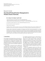
Figure 4. LCF algorithm and (b) GCF algorithm.

first have a good grasp of the working process of SIP.
Accordingly, an overview of the SIP is thus presented.

Single MA itinerary planning
Early literature of using MA in WSNs26 presented two
SIP approaches, namely, LCF and GCF. In LCF, MA
migrates to the next hop with the shortest distance to
the current node, while in GCF, MA migrates to the
next hop with the closest distance to the center of the
surveillance zone. Figure 4 shows the difference
between LCF and GCF algorithms. In Chen et al.,8
MA-based directed diffusion (MADD) was proposed.
MADD is similar to LCF but differs in which MA
selects the node as the first source that has the farthest
distance from the sink. Itinerary energy minimum for
first-source-selection (IEMF) and itinerary energy minimum algorithm (IEMA) are two algorithms were proposed by Chen et al.24 to achieve energy-efficient
itineraries. In IEMF algorithm, MA chooses the first
source node based on estimated communication cost
which extends LCF. Moreover, the impact of data
aggregation and energy efficiency are considered in
IEMF to get an energy-efficient itinerary. The second
algorithm IEMA—which is an iterative version of
IEMF—selects an optimal source node as the next
source based on estimated energy cost. However, all of
the previous works do not perform well in large-scale
sensor networks, and they suffer from several main
drawbacks as described in Bendjima and Feham.31 The
drawbacks include the following:
1.
2.
3.

Long delays when single MA has to visit hundreds of sensor nodes.

Sensor nodes in the itinerary of the MA deplete
energy faster than other nodes.
In SIP, the size of MA packet increases during
the aggregation of data from node to node as

Figure 5. Single mobile agent itinerary planning (SIP).

4.
5.

shown in Figure 5. Moreover, increase in size of
MA packet consumes higher energy especially
when MA migrates from the last node to the
sink.
Reliability reduces when the MA accumulates
an increasing amount of data.
When the MA migrates to several source nodes,
the chance of being lost increases.

Multi-MA itinerary planning
In multi-MA itinerary, several MAs dispatched from
the sink and worked in network parallel manner. Each
MA follows its assigned itinerary and visits a subset of
source nodes. In contrast to SIP, MIP overcomes the
weaknesses of using SIP, especially on a massive scale
of WSN.32,33


Qadori et al.

Figure 6. Multi-mobile agent itinerary planning (MIP).

Figure 6 shows that the multi-MAs are dispatched
to the network area with two different itineraries. In
MIP, dispatching multi-MAs decreases the packet size
of each MA, which has been defined as one of the limitations in SIP. The decrease in the MA packet size is
obtained due to the distribution of tasks that assign
each MA to an individual itinerary. Additionally, when
multi-MAs migrate to the network, each MA will visit
a sequence of nodes (a group of nodes) and then minimize the task duration (lower delay).

Determination of optimal number of MAs
in MIP
Determining the optimal number of MAs and their corresponding subsets of source nodes is a challenging
issue. Figure 7 shows the determination of the optimal
number of MAs in MIP which can be classified into
two network topologies: homogeneous network with
one sink and heterogeneous network with multiple
sinks. Most of the existing MIP algorithms have proposed a homogeneous network with one sink located at
the center of the network. Of recent MIP, a heterogeneous network with multiple sinks has been proposed
by Gavalas et al.34 In this article, the focus is on determining the optimal number of MAs in a homogeneous
network topology with one sink. The existing algorithms reviewed include tree-based MIP, central location based MIP (CL-MIP), genetic algorithm based
MIP (GA-MIP), directional angle based MIP, and
greatest information in the greater memory based MIP
(GIGM-MIP).

7

Figure 7. Classification of determination of optimal number of
MAs in MIP.

Tree-based MIP
In Mpitziopoulos et al.,33 near-optimal itinerary design
(NOID) algorithm was proposed to address the problem of calculating the number of near-optimal routes
for MAs that incrementally fuse the data as they visit
the nodes in a distributed sensor network. NOID algorithm adapts a method presented in Esau and
Williams35 namely the Esau–Williams heuristic that
was designed for the constrained minimum spanning
tree (CMST) problem in network designing. NOID
algorithm iteratively groups the sensor nodes in the network to separate sub-trees that are connected progressively to the processing element (PE) or sink. Finally,
each sub-tree is assigned to an individual MA.
Gavalas et al.36, proposed another tree based algorithm named second near-optimal itinerary design
(SNOID). This algorithm improves NOID algorithm
by taking into account the nodes communication cost.
SNOID determines the number of MAs and their itineraries they should follow by partitioning the area
around the sink or PE into concentric zones (Figure 8).
The number of nodes within the radius of the first zone
includes the PE that represents the starting points of
the itineraries of the MAs (or the number of MAs).
The first zone radius can be calculated by armax , where
a is an input parameter in the range [0, 1] and rmax is
the maximum transmission range of any sensor node.
The path of MAs itineraries starts from the inner (close
to PE) zones and proceeds to outer zones.
An improvement to the basic algorithms, NOID and
SNOID, has been obtained by a tree-based itinerary
design (TBID) algorithm presented in Konstantopoulos
et al.37 TBID not only finds the optimal number of

8

International Journal of Distributed Sensor Networks

Figure 9. GA-MIP algorithm.40

author presented an algorithm to create MIP solutions.
The main idea of the CL-MIP is to consider the solution of MIP as an iterative version of the solution of
SIP. CL-MIP algorithm includes the following four
parts:
Figure 8. Partitioning the area around PE into concentric
zones.36

1.
2.
3.

MAs, but also creates low cost itineraries for each individual MA. TBID can be suitable for WSNs with
dynamic network conditions due to its low computational complexity.
Gavalas et al.38 introduced a novel algorithm for
energy-efficient itinerary planning of MAs. This algorithm adopts a meta-heuristic method called iterated
local search (ILS) to derive the hop sequence of multiple traveling MAs over the deployed source nodes.
Like other tree-based MIP algorithms (e.g. NOID and
TBID), ILS is executed at the sink and determine the
number of itineraries (MAs) by considering a circular
zone around the sink. The nodes that are lying in the
sink zone will be the start points of each MA itinerary.
However, the difference from other previous tree-based
MIP algorithms is that ILS algorithm considers the
increasing MA size as well as the energy spent for

migrating to intermediate nodes along its itinerary.
Although NOID, SNOID, TBID, and ILS perform
better than LCF and GCF, the MA in these algorithms
(tree-based algorithms) consumes twice as much energy
due to the reverse routes that the MA take, especially
when there are huge amount of branches. Moreover,
since the itinerary of the MA is predetermined at the
PE (sink), any change in the network topology such as
a node and link failures may invalidate the migration
of MA.

CL-MIP
CL-MIP is another algorithm proposed by Chen et
al.39 to determine the proper number of MAs. The

4.

Visiting central location (VCL) selection
algorithm;
Source grouping algorithm for each MA;
Determining the source-visiting sequence using
SIP algorithm;
An iterative algorithm to ensure that a MA has
covered all the source nodes.

In CL-MIP, VCL algorithm is used to group all the
nodes of origin according to the node density (gravity
algorithm).39 The basic idea of VCL algorithm is to distribute each source nodes impact factor to other source
nodes. Let n represent the source node number; then
each source node will receive (n 2 1) impact factors

from other source nodes, and one from itself. After calculating the accumulated impact factor, the location of
the source with the largest accumulated impact factor
will be selected as a VCL. Then, the source nodes
within the radius of VCL will be assigned to the MA.
The above process will repeat until all the remaining
source nodes are assigned to an MA. Finally, the itinerary for each MA can be planned by any SIP algorithms
such as LCF, GCF, and IEMF. However, VCL algorithm assumes that the relevant source nodes are
arranged geographically distributed in several clusters,
which limits the use of the algorithm in a broad range
of applications.

GA-MIP
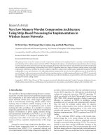
A GA-MIP was proposed in Cai et al.40 to find the
optimal number of MAs to MIP. In Figure 9, GA-MIP
is about gene that consists of source-ordering-code
(sequence array) and source grouping code (group
array). A source-ordering-code is an array that includes
segments; each segment has number of source nodes to


Qadori et al.

9

Figure 10. Angle gap grouping results.41

be visited by a particular MA. While source grouping
code is an array of numbers, with each number specifying the number of source nodes of each segment in the
source-ordering-code. The results show that the proposed GA-MIP has better performance regarding the
issues of delay and energy consumption. However, this

greedy approach may lead to a substantially suboptimal MIP solution and high computation
complexity.

Directional angle based-MIP
In this algorithm, an angle gap based MIP (AG-MIP)
is used for grouping all the source nodes in a particular
direction as a single group.41 The main idea of
direction-based MIP is to establish AG-MIP to divide
the network into sectors as shown in Figure 10. A particular angle gap threshold determines each sector.
Then, all nodes around one central location (VCL)
within this sector must be included in the same group.
Therefore, the source grouping algorithm is direction
oriented. The two nodes with minimal angel gap determine the VCL here, which differs from the previous
algorithm of VCL that presented in section ‘‘CL-MIP.’’
As a comparison with VCL, direction-based MIP
more efficiently groups the source nodes, but this algorithm may result in few isolated source nodes that are
located near the group. These isolated source nodes will
finally be considered as a new sector after several iterations. Moreover, how to find an optimal angle gap
threshold in this approach is still an open issue.
Wang et al.42 improve the previous work presented
in Cai et al.41 by proposing an algorithm entitled directional source grouping based MIP (DSG-MIP). This
algorithm partitions the network area into sector zones

Figure 11. Directional source grouping algorithm
(DSG-MIP).42

whose centers are the sensor nodes within the radius of
the sink node or PE. Figure 11 shows that the size of
the PE zone can be determined by the same algorithm
presented in SNOID algorithm, aRmax where R is the

maximum transmission range, and a is an input parameter in the range [0, 1]. Then, the sensor node within
this zone represents the starting points of each MA. By
controlling the value of parameter a, the number of
MAs can be determined. As shown in Figure 11, after
three iterations, there are only two isolated source
nodes remaining, u and v. These isolated source nodes
(u and v) are simply grouped and assigned to the last


10

International Journal of Distributed Sensor Networks

itinerary with node f as the starting point. The contribution of DSG-MIP was that those isolated source
nodes can be inserted into existing itineraries one by
one according to the metric of shortest distance to the
itinerary. Then, the incremental cost of the formed itinerary is minimized. However, inserting the isolated
source nodes into existing itineraries could increase the
delay of the MA especially when the isolated source
nodes are located far away from the existing itineraries.
Moreover, similar to AG-MIP algorithm, DSG-MIP
algorithm is unable to find the optimal gap threshold.

Greatest information in the GIGM-MIP
In the previous algorithms of determining the optimal
number of MAs, most of the itinerary planning algorithms are based only on geographic information. The
author in Aloui et al.43 proposed a new MIP algorithm
called GIGM-MIP to determine the number of MAs
with their source nodes grouping. This algorithm is
based not only on geographic information, but also on

the amount of data provided by each source node.
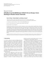
GIGM-MIP algorithm is divided into three parts: (1)
Partitioning the network into a set of partitions based
on geographical information and each partition can
have several MAs. (2) Finding out the necessary number of MAs and their groups of nodes while considering the data size provided by each source node. (3)
Defining the itinerary plan for each MA to visit the
source nodes. As shown in Figure 12, the network is
partitioned into two partitions, and one of the partitions has more than one MA.
Partitioning the network in GIGM-MIP algorithm
is established according to the distance among the sensor nodes (nodes closest to each other are grouped
together). K-Means algorithm is used to partition the
network into K clusters. However, although K-Means
is an efficient algorithm for a large-scale network, some
clusters K must be specified. In MIP, the number of
clusters has to be determined optimally according to
several parameters such as the distance between nodes,
density, and energy of nodes.

Discussion and future research directions
The use of MIP for data gathering purpose in WSNs
achieves a significant improvement in minimizing the
energy consumption and thus prolongs the lifetime of
the network. By grouping the sensor nodes into several
groups (partitions), MIP decreases the MA packet size
by visiting a group of sensor nodes individually.
Furthermore, due to the distribution of the given tasks,
the task duration is decreased when MIP is applied.
However, with these advantages of MIP, grouping the
sensor nodes and finding the optimal itinerary of each
MA to visit the given set of the sensor nodes is a

Figure 12. Partitioning the network by GIGM-MIP algorithm.43

challenging issue. In section ‘‘Determination of optimal
number of MAs in MIP,’’ the reviewed approaches
have proposed different algorithms to find an optimal
grouping of the sensor nodes. Table 1 compares the
proposed algorithms in terms of the parameters that
were used to find the optimal grouping of the sensor
nodes. Most of the MIP39,41,42 algorithms used the
nodes density as the main factor to group the visiting
nodes, while other algorithms used different parameters
such as nodes radius and communication cost.33,36,37 In
Aloui et al.,43 the number of groups (partitions) is
manually specified, but the number of MAs is determined by the data size in each partition; therefore, each
partition may have several MAs. However, the optimal
partitioning of the network has to take into account
several parameters such as density, communication
cost, energy, and data size at each sensor.
Based on what is mentioned above, some future
research directions are highlighted as follows.

Efficient source nodes grouping of MIP
Grouping the source nodes is the key challenge in MIP.
An effective algorithm for source nodes grouping will
result in efficient energy consumption. The previous
algorithms of grouping the source nodes that were
reviewed have some weaknesses. Therefore, it would be
interesting on how to find out a way of group the
source nodes efficiently. X-Means algorithm presented

in Pelleg and Moore44 could be suitable to produce an
efficient source nodes grouping. In K-Means algorithm
presented in Aloui et al.,43 the number of groups (clusters) has to be specified manually by the user where in
X-Means algorithm, the number of groups, is optimally
obtained.


MIP: multi-agent itinerary planning; MA: mobile agent; GA-MIP: genetic algorithm based MIP; GIGM-MIP: greater memory based MIP; CL-MIP: central location based MIP; AG-MIP: angle gap based MIP; DSGMIP: directional source grouping based MIP; ILS: iterated local search; TBID: tree-based itinerary design; SNOID: second near-optimal itinerary design; NOID: near-optimal itinerary design; VCLs: visiting
central locations.

Optimal number of MAs
Number of MAs is determined
by the data size in each partition
Distance between the sensor nodes
Distance between the sensor nodes
An initial number of MAs
Number of partitions is manually specified

Static
Static

Number of partitions
Number of partitions
Number of partitions
Node radius
Node radius and communication cost
Nodes density
Number of nodes within the radius of the PE
Number of nodes within the radius of the PE
Number of VCLs

NOID33
SNOID,36 TBID,37 and ILS38
CL-MIP,39 AG-MIP,41
and DSG-MIP42
GA-MIP40
GIGM-MIP43

Number of MAs is determined by
Parameters used for partitioning

Static
Static
Static

11

Number of partitions is determined by
Algorithm

Table 1. A comparison of MIP algorithms in terms of parameters used to find the optimal number of partitions and MAs.

Itinerary planning
of MA

Qadori et al.

Dynamic itinerary of MIP
In MIP planning algorithm, most of the proposed solutions assume that the itinerary of each MA is determined at the sink node, which means the MA is
carrying a static itinerary. In this case, any change in

the network topology due to node mobility or node
failures (such as energy depletion) could affect the
migration of MA. The migration of MA has to be
dynamic and more intelligent, such that the MA migration is decided at each visited sensor node. Therefore, it
is recommended that the MA packet carries an alternative source nodes list together with the list that is predetermined at the sink. The alternative source nodes list
will contain the nearest neighbor node of each next hop
node. This proposed solution might increase the MA
packet size slightly. The added alternative source nodes
list (to the MA packet) could increase the time of MA
hop migration at each node. While this solution consumes energy and time, on the other hand, however, it
is beneficial and applicable for dynamic migration
(such as target tracking applications).

Collaboration of multi-MAs in MIP
As long as several MAs are dispatched and work in
parallel for data gathering in MIP, each MA assigned
to individual data gathering task. It is recommended
that each MA collaborates with other MAs to distribute the assigned tasks. In the previous MIP algorithms, each individual MA itinerary has its own source
nodes list and the number of source nodes of each MA
itinerary is varied from one to another. Moreover, each
MA starts its migration from the sink and returns back
again to the sink. For instance, in Figure 12, one of the
clusters has two itineraries and one of these itineraries
has fewer source nodes than the second one. From this
point, it is suggested that such source nodes should collaborate with other MAs that have more source nodes
to visit. This collaboration could decrease the overall
task duration of MAs and balance the data size carried
among all MAs. Thus, a high QoS will be provided
while taking into account the task duration and energy
consumption.

MA data security
The data carried by the MA are assumed to be secure
with the MA migration. Since the migration of the MA
is done by several hops among the sensor nodes, the
limited available energy at these sensor nodes will affect
the MA migration and the data carried by the MA
may be lost. Therefore, it is recommended to use any
of the compression algorithms to compress the data
accumulated by each MA. The compression code with
an encryption key should be carried by the MA so that


12
once the MA reaches the source node, it compresses
the accumulated data and then later when the MA
finishes its task, the encrypted data accumulated will be
decrypted at the sink.

International Journal of Distributed Sensor Networks

3.

4.

Conclusion
In this article, we analyzed the background of data
gathering in WSNs using MA-based model. The main
goal of this article was to show the impact of using
MIP for data gathering in WSNs. It has been proven

that using MIP for data gathering achieves a significant
improvement in minimizing the energy consumption.
MIP overcomes the weakness of SIP in terms of task
duration and MA packet size, but on other hand, MIP
still has some drawbacks. In general, it seems that finding the optimal number of MAs in MIP is considered
as a non-deterministic polynomial (NP)-hard problem.
Therefore, this article reviewed and discussed the existing algorithms that have identified in the literature to
determine the optimal number of MAs in MIP.
Particularly, we analyzed the most adapted algorithms:
tree-based MIP, CL-MIP, GA-MIP, directional angle
based MIP, and GIGM-MIP. This article showed that
most of the algorithms used one parameter to find the
optimal number of MAs in MIP without utilizing other
parameters which could give efficient results. More significantly, this article demonstrated that these algorithms have not considered the security of the data
gathered by the MA.
Consequently, the limitations of each proposed algorithm were shown and new directions are provided for
future research. In particular, we have started working
on the two of the proposed approaches: efficient source
nodes grouping of MIP (with X-means algorithm) and
collaborative of multi-MAs in MIP. The results are promising and will be presented in future articles.
Declaration of conflicting interests

5.

6.

7.

8.

9.

10.

11.
12.

13.

14.

The author(s) declared no potential conflicts of interest with
respect to the research, authorship, and/or publication of this
article.

15.

Funding

16.

The author(s) received no financial support for the research,
authorship, and/or publication of this article.

References
1. Sarangi S and Thankchan B. A novel routing algorithm
for wireless sensor network using particle swarm optimization. IOSR-JCE 2012; 4(1): 26–30.
2. Jayram BG and Ashoka DV. Merits and demerits of
existing energy efficient data gathering techniques for

17.

18.

19.

wireless sensor networks. Int J Comput Appl 2013; 66(9):
15–22.
Cheng C-T, Tse CK and Lau F. A delay-aware data collection network structure for wireless sensor networks.
IEEE Sens J 2011; 11(3): 699–710.
Dhawan H and Waraich S. A comparative study on
leach routing protocol and its variants in wireless sensor
networks: a survey. Int J Comput Appl 2014; 95(8), http:
//research.ijcaonline.org/volume95/number8/pxc3896454.
pdf
Tan H and Ibrahim K. Power efficient data gathering
and aggregation in wireless sensor networks. ACM SIGMOD Rec 2003; 32(4): 66–71.
Saad W, Han Z, Debbah M, et al. Coalitional game theory for communication networks. IEEE Signal Proc Mag
2009; 26(5): 77–97.
Levis P and Culler D. Mate´: a tiny virtual machine for
sensor networks. ACM Sigplan Notices 2002; 37(10):
85–95.
Chen M, Kwon T, Yuan Y, et al. Mobile agent-based
directed diffusion in wireless sensor networks. EURASIP
J Appl Si Pr 2007; 2007(1): 219.
Gupta GP, Misra M and Garg K. Multiple mobile
agents based data dissemination protocol for wireless
sensor networks. In: Meghanathan N, Chaki N and
Nagamalai D (eds) Advances in computer science and
information technology: networks and communications,

2012, pp.334–345. Berlin, Heidelberg: Springer.
Paul T and Stanley KG. Data collection from wireless
sensor networks using a hybrid mobile agent-based
approach. In: 2014 IEEE 39th conference on local computer networks (LCN), Edmonton, AB, Canada, 8–11
September 2014, pp.288–295. New York: IEEE.
Chen M, Kwon T, Yuan Y, et al. Mobile agent based
wireless sensor networks. J Comput 2006; 1(1): 14–21.
Qi H, Wang X, Sitharama Iyengar S, et al. Multisensor
data fusion in distributed sensor networks using mobile
agents. In: Proceedings of 5th international conference on
information fusion, 2001, pp.11–16.
Yuan L, Wang X, Gan J, et al. A data gathering algorithm based on mobile agent and emergent event-driven
in cluster-based WSN. J Network 2010; 5(10): 1160–1168.
Lingaraj K and Aradhana D. A survey on mobile agent
itinerary planning in wireless sensor networks. Int J Comput Commun Technol 2012; 3(6): 51–56.
Chen M, Gonzalez S and Leung V. Applications and
design issues for mobile agents in wireless sensor networks. IEEE Wirel Commun 2007; 14(6): 20–26.
Xu Y and Qi H. Mobile agent migration modeling and
design for target tracking in wireless sensor networks. Ad
Hoc Netw 2008; 6(1): 1–16.
Dong M, Ota K, Lin M, et al. UAV-assisted data gathering in wireless sensor networks. J Supercomput 2014;
70(3): 1142–1155.
Di Francesco M, Das SK and Anastasi G. Data collection in wireless sensor networks with mobile elements: a
survey. ACM T Sensor Network 2011; 8(1): 7.
Gowri K, Chandrasekaran M and Kousalya K. A survey
on energy conservation for mobile-sink in WSN. Int J
Comput Sci Inform Tech 2014; 5(6): 7122–7125.


Qadori et al.

20. Chen Y, Chen J, Zhou L, et al. A data gathering
approach for wireless sensor network with quadrotorbased mobile sink node. In: Wang R and Xiao F (eds)
Advances in wireless sensor networks, 2012, pp.44–56.
Berlin, Heidelberg: Springer.
21. Sugihara R and Gupta RK. Optimal speed control of
mobile node for data collection in sensor networks. IEEE
T Mobile Comput 2010; 9(1): 127–139.
22. Vukasinovic I, Babovic Z and Rakocevic O. A survey on
the use of mobile agents in wireless sensor networks. In:
2012 IEEE international conference on industrial technology (ICIT), Athens, 19–21 March 2012, pp.271–277.
New York: IEEE.
23. Shakshuki EM, Malik H and Sheltami T. WSN in cyber
physical systems: enhanced energy management routing
approach using software agents. Future Gener Comp Sy
2014; 31: 93–104.
24. Chen M, Leung V, Mao S, et al. Energy-efficient itinerary
planning for mobile agents in wireless sensor networks.
In: IEEE international conference on communications
(ICC’09), Dresden, June 2009, pp.1–5. New York: IEEE.
25. Wu Q, Rao NSV, Barhen V, et al. On computing mobile
agent routes for data fusion in distributed sensor networks. IEEE T Knowl Data En 2004; 16(6): 740–753.
26. Qi H and Wang F. Optimal itinerary analysis for mobile
agents in ad hoc wireless sensor networks. P IEEE 2001;
147–153, />27. Venetis IE, Pantziou G, Gavalas D, et al. Benchmarking
mobile agent itinerary planning algorithms for data
aggregation on WSNs. In: 2014 sixth international conference on ubiquitous and future networks (ICUFN), Shanghai, China, 8–11 July 2014, pp.105–110. New York:
IEEE.
28. Gupta GP, Misra M and Garg K. Energy and trust aware
mobile agent migration protocol for data aggregation in
wireless sensor networks. J Netw Comput Appl 2014; 41:

300–311.
29. Kallapur PV and Chiplunkar NN. Topology aware
mobile agent for efficient data collection in wireless sensor networks with dynamic deadlines. In: 2010 international conference on advances in computer engineering
(ACE), Bangalore, India, 20–21 June 2010, pp.352–356.
New York: IEEE.
30. Tsai HW, Chu CP and Chen TS. Mobile object tracking
in wireless sensor networks. Comput Commun 2007; 30(8):
1811–1825.
31. Bendjima M and Feham M. Optimal itinerary planning
for mobile multiple agents in WSN. Int J Adv Comput Sci
Appl 2012; 3(11): 13–19.
32. Wang X, Chen M, Kwon T, et al. Multiple mobile agents’
itinerary planning in wireless sensor networks: survey and
evaluation. IET Commun 2011; 5(12): 1769–1776.

13
33. Mpitziopoulos A, Gavalas D, Konstantopoulos C, et al.
Deriving efficient mobile agent routes in wireless sensor
networks with NOID algorithm. In: IEEE 18th international symposium on personal, indoor and mobile radio
communications (PIMRC 2007), Athens, 3–7 September
2007, pp.1–5. New York: IEEE.
34. Gavalas D, Venetis IE, Konstantopoulos C, et al. Mobile
agent itinerary planning for WSN data fusion: considering multiple sinks and heterogeneous networks. Int J
Commun Syst. Epub ahead of print 1 September 2016.
DOI: 10.1002/dac.3184.
35. Esau LR and Williams KC. On teleprocessing system
design: part ii a method for approximating the optimal
network. IBM Syst J 1966; 5(3): 142–147.
36. Gavalas D, Pantziou G, Konstantopoulos C, et al. New
techniques for incremental data fusion in distributed sensor networks. In: Proceedings of the 11th Panhellenic conference on informatics (PCI 2007), Patras, 18–20 May

2007, pp.599–608. CiteSeerX, The Pennsylvania State
University, />37. Konstantopoulos C, Mpitziopoulos A, Gavalas D, et al.
Effective determination of mobile agent itineraries for
data aggregation on sensor networks. IEEE T Knowl
Data En 2010; 22(12): 1679–1693.
38. Gavalas D, Venetis IE, Konstantopoulos C, et al.
Energy-efficient multiple itinerary planning for mobile
agents-based data aggregation in WSNs. Telecommun
Syst 2016; 63: 531–545.
39. Chen M, Gonzalez S, Zhang Y, et al. Multi-agent itinerary planning for wireless sensor networks. In: Bartolini
N, Nikoletseas S, Sinha P, et al. (eds) Quality of service in
heterogeneous networks, 2009, pp.584–597. Berlin, Heidelberg: Springer.
40. Cai W, Chen M, Hara T, et al. A genetic algorithm
approach to multi-agent itinerary planning in wireless
sensor networks. Mobile Netw Appl 2011; 16(6): 782–793.
41. Cai W, Chen M, Wang X, et al. Angle gap (AG) based
grouping algorithm for multi-mobile agents itinerary
planning in wireless sensor networks. In: Proceedings of
Symposium of the Korean Institute of communications and
Information Sciences, Seoul, Republic of Korea, 2009, vol.
11, pp. 305–306. Korea Institute of Communication Sciences.
42. Wang J, Zhang Y, Cheng Z, et al. EMIP: energy-efficient
itinerary planning for multiple mobile agents in wireless
sensor network. Telecommun Syst 2015; 62: 93–100.
43. Aloui I, Kazar O, Kahloul L, et al. A new itinerary planning approach among multiple mobile agents in wireless
sensor networks (WSN) to reduce energy consumption.
Int J Comm Network Inform Secur 2015; 7(2): 116.
44. Pelleg D and Moore AW. X-means: extending k-means
with efficient estimation of the number of clusters. ICML
2000; 1: 1–8.