Báo cáo hóa học: " Research Article Efficient Data Association in Visual Sensor Networks with Missing Detection" ppt

Hindawi Publishing Corporation
EURASIP Journal on Advances in Signal Processing
Volume 2011, Article ID 176026, 25 pages
doi:10.1155/2011/176026
Research Article
Efficient Data Association in Visual Sensor Networks with
Missing Detection
Jiuqing Wan and Qing yun Liu
Department of Automation, Beijing University of Aeronautics and Astronautics, Beijing 100191, China
Correspondence should be addressed to Jiuqing Wan,
Received 26 October 2010; Revised 16 January 2011; Accepted 18 February 2011
Academic Editor: M. Greco
Copyright © 2011 J. Wan and Q. Liu. This is an open access article distributed under the Creative Commons Attribution License,
which permits unrestricted use, distribution, and reproduction in any medium, provided the original work is properly cited.
One of the fundamental requirements for visual surveillance with Visual Sensor Networks (VSN) is the correct association of
camera’s observations with the tracks of objects under tracking. In this paper, we model the data association in VSN as an
inference problem on dynamic Bayesian networks (DBN) and investigate the key problems for efficient data association in case of
missing detection. Firstly, to deal with the problem of missing detection, we introduce a set of random variables, namely routine
variables, into the DBN model to describe the uncertainty in the path taken by the moving objects and propose the high-order
spatio-temporal model based inference algorithm. Secondly, for the problem of computational intractability of exact inference, we
derive two approximate inference algorithms by factorizing the belief state based on the marginal and conditional independence
assumptions. Thirdly, we incorporate the inference algorithm into EM framework to make the algorithm suitable for the case when
object appearance parameters are unknown. Simulation and experimental results demonstrate the effect of the proposed methods.
1. Introduction
Consisting of a large number of cameras with nonover-
lapping field of view, Visual Senor Networks (VSNs) have
been frequently used for surveillance of public locations
such as airports, subway stations, busy streets, and pub-
lic buildings. The visual nodes in VSN are not working
independently; instead, they can transmit information to a
processing centre or communicate with each other. Typically,

in the region covered by the VSN there are several moving
objects (persons, cars, etc.), presenting in one camera at
a certain time and reappearing in another after a certain
period. The visual information captured by VSN can be
used for interpreting and understanding the activities of
moving objects in the monitored region. One of the basic
requirements for achieving these goals is to accurately
associate the observations produced by the visual node with
the track of each object of interest. It is interesting to
note that a similar problem also arise, in the multitargets
tracking (MTT) research, where the goal is to associate the
several distinct track segments produced by the same target.
For example, Yeom et al. [1] proposed a track segments
association technique for improving the track continuity in
airborne early warning system using discrete optimization
on the possible matching pairs of track segments given by
forward prediction and backward retrodiction. However, the
target motion model used in multitargets tracking is not
available in VSN, as large blind regions always exist between
camera nodes.
Appearance information can be used to associate the
observation with object’s track, provided the characteristics
of the object appearance are known or have been learnt.
However, the appearance observations of the same object
generated by different visual nodes may vary dramatically
due to changes in the illumination of scene or the pho-
tometric property of cameras. Despite the huge amount
of effort to overcome these difficulties using intercamera
color calibration [2] or appearance similarity models [3], the
association performance based solely on appearance cues is

still unsatisfactory. On the other hand, the spatiotemporal
observations such as the time of object visiting the specific
camera and the location of that camera, combined with
the structural knowledge of monitored region, can be used
to improve the accuracy of data association. Representing
the prior knowledge of the object’s characteristics and the
monitored region by a graphical probabilistic model, the data
2 EURASIP Journal on Advances in Signal Processing
association problem can be solved by Bayesian inference [4–
8].
However, the introduction of spatiotemporal informa-
tion greatly complicates the association problem in the
following two aspects. First, as the spatiotemporal obser-
vations of the same object from cameras in the VSN
are inter-dependent, and the number of the association
hypothesis usually increases exponentially with the accu-
mulation of observations, rendering the exact inference
algorithm intractable. In fact, intractability is an intrinsic
property of the data association problems, no matter in
VSN or in traditional multitargets tracking [9]. In traditional
MTT community, data association problem can be solved
by approximate algorithms such as Multiple Hypothesis
Tracking (MHT) [10], Probabilistic Multiple Hypothesis
Tracking (PMHT) [11], and Joint Probability Data Asso-
ciation (JPDA) [12]. However, the assumption of motion
smoothness in traditional MTT is not available in VSN.
Second, the performance of the spatiotemporal observation-
based association algorithms is more vulnerable than that of
the appearance-based methods to the unreliable detection,
including false measurement and missing detection. In

practice, unreliable detection is difficult to avoid due to the
bad observation condition or the occlusion of the object of
interest. The problem of false measurement can be alleviated
by deleting the observations with low likelihood. However,
missing detection is more difficult to handle as it is not
easy to know whether an object is miss detected based
on the information on a single camera. Moreover, missing
detection can result in very low posterior probability of the
true object trajectory, as most spatiotemporal model-based
inference algorithms rely on the assumption that the object
can be detected reliably. Therefore, in this paper we focus our
attention on the problem of missing detection and assume
that there is no false or clutter measurement.
In fact, unreliable detection may also be encountered
in traditional MTT applications such as low elevation sea
surface target (LESST) tracking, where the SNR at receiver
can be dramatically reduced due to the presence of multipath
fading. For example, Wang and Mu
ˇ
sicki [13] present a series
of integrated PDA type filters which can output not only
target state estimate but also a measure of track quality,
taking into account the existence of target and the SNR of
sensor. Godsill and Vermaak [14] deal with the problem
of unreliable detection by incorporating a new observation
model based upon a Poisson assumption for both targets and
clutter into the variable rate particle filter framework.
In this paper, we present a novel method for data associa-
tion in VSN based jointly on appearance and spatiotemporal
observation, overcoming the difficulties mentioned above.

After a brief review of the related works, in Section 3 we
model the data association problem with dynamic Bayesian
networks, where a set of routing variables are introduced to
overcome the problem of missing detection. In Section 4 we
present the forward and backward exact inference algorithms
for data association in DBN and show their intractability
when the number of objects grows. To reduce the com-
putational burden, in Section 5 we derive two kinds of
approximation inference algorithms by factorizing the joint
probability distribution based on different independence
assumptions. To apply the algorithms when objects appear-
ancemodelisunavailable,inSection 6 we incorporate the
proposed inference algorithms into EM framework, where
the data association and parameter estimation problems are
solved simultaneously. Simulation and experimental results
are presented in Section 7 and conclusions are given in
Section 8.
2. Related Works
The data association in VSN can be considered as the
process of partitioning the set of observations collected by
all cameras in VSN into several exhaustive and exclusive
subsets, such that the observations belonging to each subset
are believed to come from a single object. Then the data
association problem can be solved by finding the partition
with the highest posterior probability. Usually, the joint
probability of partitions and observations is encoded by
some graphical model. Pasula et al. [4] proposed a graphical
model to represent the probabilistic relationships between
the assignments variables, observations, and the hidden
intrinsic and dynamic states of the objects under tracking.

The introduction of hidden states in [4] avoids the com-
binatorial explosion in the number of the model param-
eters. Kim et al. [7] provided a first-order Markov model
describing the activity topology of the camera networks,
with so-called super nodes of the ordered entry-exit zone
pairs and directional edges weighted by the likelihood of
transition between cameras and the travel time. The model
is superior in distinguishing traffic patterns compared with
conventional activity topology models. Zajdel and Kr
¨
ose
[6] used dynamic Bayesian networks (DBNs) as generative
model of observations from a single object. Every partition
of the entire observations translates into a specific structure
of a larger network that comprised multiple disconnected
DBNs. The authors provided an EM-like approach to select
the most likely structure and learn the model parameters.
In the works mentioned above, although the association
performance has been studied as a function of the increasing
observation noise, none of them considered the problem
of missing detection explicitly in their models. Van De
Camp et al. [8] modeled the behavior of a single person
by a Hidden Markov Model (HMM), with the hidden state
representing the location of the person under tracking. In
[8], each camera was represented by two states to be able to
model the case of a person passing a camera without being
detected.
In the above works, the complexity nature of data
association reflects in the intractability of the partition space,
which expands combinatorially with the number of observa-

tions. In [4, 7], the authors resort to Markov Chain Monte
Carlo (MCMC) sampling method to represent the partition
space by a set of samples with high posterior probability.
Although MCMC-based method has been widely used in
data association [15] and object tracking [16]problemsand
is simple to implement, it is usually computational intensive
and rather sensitive to initial samples. In [6], the authors
EURASIP Journal on Advances in Signal Processing 3
approximate the full partition space by a Multiple Hypothesis
Tracker- (MHT-) like approach, preserving the several most
likely partitions and extending each partition with the
subsequent observations. However, it is questionable if the
true partition is also discarded as unlikely ones by a simple
threshold value.
An alternative way to solve data association problem in
VSN is to assume an imaginary label for each observation,
indicating which object it comes from. As the label cannot
be observed, it is treated as a hidden random variable. By
inferring the posterior distribution of the imaginary label
based on all available evidences, the object corresponding
to each observation can be determined without explicit
enumeration of the partitions of observations. In [5],
the imaginary label is identified by probabilistic clustering
the observations with an extension of Gaussian Mixture
Model (GMM), where a set of hidden pointer variables
are introduced to capture Markov dependencies between
spatiotemporal observations generated by the same Gaussian
kernel. However, the state space of the auxiliary hidden
variables grows exponentially with the number of objects.
This makes it very difficult to marginalize these variables

out. The author solves the problem by Assumed Density
Filtering (ADF) algorithm [17], where the joint distribution
is replaced with a factorial approximation. Following the
same way, in [18] the author presents a hybrid graphical
model with discrete states identifying objects labels and
continuous states underlying appearance and spatiotemporal
observations. The model parameters are treated as a part
of the state, allowing them to be learnt automatically with
Bayesian inference. However, the inference is still difficult in
that the posterior joint distribution take the form of mixtures
of an intractable number of components due to the inherent
association ambiguity.
In our work we also use the auxiliary pointer variables
in [5, 18] to indicate the last observation of each object
directly before the current one, but our work is differentiated
from them in the following two aspects. First, the model in
[5, 18] is based on the assumption that the objects cannot
be miss detected by cameras. If this assumption is violated,
as is often the case in practice, the association accuracy
of the algorithm decreases significantly. In our work we
tackle this problem by introducing another set of hidden
variables indicating the path taken by the object from one
camera to another. By considering all possible paths with
limited length between camera nodes, the robustness of
the algorithm against missing detection is greatly improved.
Second, in [5, 18] the author factorized the joint distribution
into the product of distributions of the label variable and
single pointer variable to avoid the combinatorial explosion
of state space. However, as the Markov transition process
of the pointer variable is deterministic, the mixing rate

of the process is zero. Theoretically, for this case the
accumulated approximation error bound is infinite [17]. In
contrast, we propose another scheme of factorization of the
joint distribution based on the conditional independence
between the pointer variables given the imaginary label.
The proposed approximate inference demonstrates better
association performance in simulation and experiment.
There are also other ways to solve the data association
problems in VSN. It is very interesting to note that Loy et
al. [19] proposes a novel approach for modeling correlations
between activities observed by multiple nonoverlapping
cameras. After decomposing each camera view into semantic
regions according to the similarity of local activity patterns,
the correlation structure of the semantic regions is discovered
automatically by Cross Canonical Correlation Analysis. The
resulting correlation structure can be used to improve data
association performance by reducing the searching space and
resolving the ambiguities arisen from similar visual features
presented by different objects. Song and Roy-Chowdhury
[20] propose a multiobjective optimization framework
combining short-term feature correspondences across the
cameras with long-term feature dependency models. The
overall solution strategy involves adapting the similarities
betweenfeaturesobservedatdifferent cameras based on
the longterm models and finding the stochastically optimal
path for each object. Based on activity topology graph, Ket-
tneker and Zabih [21] transform the multicamera tracking
problem into a linear assignment problem, which can be
solved in polynomial time. However, since the weighted
assignment algorithm uses correspondences between only

two observations, other useful information such as the
length and the frequency of path should be decomposed
into “between-two-cameras” terms with a decomposable
assumption. A high-order transition model can be used to
associate the observations [22], but it turns the problem into
multidimensional assignment problem.
3. Bayesian Modeling
In this section we formulate the problem of data association
in VSN with missing detections and show that it can be
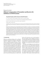
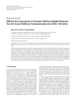
solved by inference on dynamic Bayesian networks. Suppose
that K objects are moving in the region monitored by M
cameras, as shown in Figure 1.WeuseA
={a
uv
}
M
u,v
=1
to
denote the parameter matrix of the VSN, each element of
A consists of three components, that is, a
uv
= (π
uv
, t
uv
, s
uv
),
π

uv
is the transition probability of object moving from
camera u to camera v,andπ
uv
= 0 means there is
no edge between camera u and v. t
uv
and s
uv
are the
mean and variance of the traveling time between u and v,
respectively. Since we focus on camera-to-camera trajectory,
we do not analyze the maneuvers of an object within the
FOV of a single camera. The duration of object’s presence
in a viewing field is assumed to be significantly shorter
than the travel times between cameras. Therefore, we will
represent the interval within a camera field as a single
timestamp and derive a “virtual” observation y
i
={o
i
, d
i
, c
i
},
automatically or manually, from the sequence of frame
captured by the camera once an object passed by. Here, o
i
is the measurement of object appearance characteristics, and

it can be the average of measurements on different frames,
or just the measurement on a single fame; d
i
is the time
when observation was made, and it can be the time instant
of object entry or departure, or the median of them; c
i
is the
camera at which the observation was made. All the generated
4 EURASIP Journal on Advances in Signal Processing
a
b
c
d
e
f
g
h
i
j
Figure 1: Topology of visual sensor networks. Circles depict
cameras; edges depict path between cameras.
observations are collected to a data processing center and
reordered according to their generating time, that is, d
i
<d
j
if i<jforanytwoobservationsy
i
and y

j
.
For each observation we introduce a labeling random
variable x
i
∈{1, , K}; x
i
= k indicates that the
observation y
i
is originated from the object k. In addition,
we introduce another set of auxiliary random variables z
i
=
{
z
(k)
i
}
K
k
=1
,eachz
(k)
i
∈{0, ,i − 1} indicates which of the
observations y
0
, , y
i−1

was the last observation of object
k directly before the observation y
i
,andz
(k)
i
= 0means
y
i
is the first observation of object k.Bothx
i
and z
i
are
unobserved and considered as hidden states to be estimated
based on available observations. The goal of data association
is to calculate the marginal posterior distribution of x
i
, that
is, p(x
i
| y
0:i
). In this section we first define the state
transition model and observation model for the case of
reliable detection and then introduce the routing random
variables to accommodate the missing detections; finally we
express the generating process of the observations sequence
compactly with dynamic Bayesian networks.
3.1. State Transition Model. Based on the definition of

hidden state variable x
i
and z
i
, it is reasonable to assume
that the state evolve as a first-order Markov process. The state
transition model can be written as
p
(
x
i
, z
i
| x
i−1
, z
i−1
)
= p
(
x
i
)
f

z
i
| x
i−1
= k, z

(k)
i
−1
= l

. (1)
The prior probability p(x
i
) can be assumed to follow a
uniform distribution if no prior knowledge about x
i
is
available. It should be noticed in above model that if x
i−1
and
z
i−1
aregiven,thevalueofz
i
is determined. Specifically, if the
observation y
i−1
is produced by object k, that is, x
i−1
= k,
then z
(k)
i
takes value of i − 1 and other components in z
i

remain unchanged, that is,
z
(k)
i
= z
(k)
i
−1
[
x
i−1
/
=k
]
+
(
i − 1
)
[
x
i−1
= k
]
,(2)
where [g]
≡ 1(0) if and only if the logical variable g is true
(false).
3.2. Observation Model. The observation includes appear-
ance measurement and spatiotemporal measurement. We
assume that they are conditionally independent given the

current state, and both of them follow Gaussian distribution.
Theappearanceobservationmodelofagivenobjectis
p
(
o
i
| x
i
= k
)
= N

o
i
; μ
k
, σ
2
k

,(3)
where μ
k
and σ
2
k
are mean and variance of the appearance of
the kth object. The appearance observation is independent of
the state z
i

. The spatiotemporal observation is dependent on
x
i
, z
i
and past observations y
0:i−1
, as follows:
p

d
i
, c
i
| x
i
= k, z
(k)
i
= l, y
0:i−1

=
p

d
i
| x
i
= k, z

(k)
i
= l, d
l
, c
l
= u, c
i
= v

×
p

c
i
= v | x
i
= k, z
(k)
i
= l, d
l
, c
l
= u

=
⎧
⎨
⎩

c, l = 0,
π
uv
N
(
d
i
−d
l
; t
uv
, s
uv
)
, l
/
=0.
(4)
Note that the spatiotemporal observation only depends on
z
(k)
i
if x
i
= k. As the observation y
0
is undefined, we set the
likelihood in the case of l
= 0toaconstantvaluec.
3.3. Missing Detection. At each monitoring camera, missing

detection is unavoidable due to the unfavourable observing
conditions. When the object of interest is miss detected, the
true trajectory of that object cannot be expressed in terms
of any sequence of state variable z
(k)
i
, i = 1, , N. This will
introduce unpredictable errors in the likelihood evaluation
according to (4) and hence deteriorate the performance of
data association algorithm significantly. To deal with this
problem, we introduce another set of random variable,
namely, routing variables ω
i
={ω
(u,v)
i
}
M
u,v
=1
, to describe the
uncertainty in the object moving path. The routing variable
ω
(u,v)
i
indicates the path with maximum length of L taken by
an object moving from camera u to v.Itisadiscreterandom
variable taking values in the set
{1, , R
L

uv
},whereR
L
uv
is the
number of path form u to v not longer than L. The path
length here is the number of camera nodes between u and v;
L
= 0 means that u and v are connected directly. The choice
of L depends on the rate of missing detection, larger L for
a higher missing detection rate, and vice versa. ω
i
is a very
large set of variables as it enumerates all pairing of cameras in
the VSN. It seems that this will bring a huge computational
burden in the inference computation. Fortunately, it turns
out in Section 4 that most of the routing variables can
be summed out during inference and the introduction of
routing variable increases the computational burden very
slightly.
EURASIP Journal on Advances in Signal Processing 5
y
0
y
1
y
2
y
3
x

1
x
2
x
3
Z
1
1
z
1
2
z
1
3
z
K
1
z
K
2
z
K
3
w
1
w
2
w
3
.

.
.
.
.
.
.
.
.
(a)
w
i
z
i
x
i
o
i
d
i
c
i
(b)
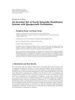
Figure 2: (a): Dynamic Bayesian networks model; (b) dependency in a single time slice. Solid arrows depict stochastic dependency; dashed
arrows depicted deterministic one. Squares depict discrete random variables; circles depicted continuous ones.
p(x
i−1
|y
0:i−1
)
P(z

(k)
i
−1
|y
0:i−1
)
p(x
i−1
, z
(k)
i
−1
|y
0:i−1
)
p(x
i−1
, z
(j)
i
−1
, z
(k)
i
−1
|y
0:i−1
)
p(x
i

, z
(j)
i
, z
(k)
i
|y
0:i
)
i
−1 i
Belief state
Intermediate
distributions
p(x
i
|y
0:i
)
p(z
(k)
i
|y
0:i
)
p(x
i
, z
(k)
i

|y
0:i
)
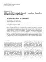
Figure 3: Belief state propagation in forward pass of Approximate
inference I. We only need to maintain the belief state the interme-
diate distributions can be calculated based on the independence
assumptions when necessary, as indicated by the arrows within each
time slice.
p(x
i−1
|y
0:i−1
)
p(x
i−1
, z
(k)
i
−1
|y
0:i−1
)
p(x
i−1
, z
(j)
i
−1
, z
(k)

i
−1
|y
0:i−1
)
p(x
i
, z
(j)
i
, z
(k)
i
|y
0:i
)
i
−1 i
Belief state
Intermediate
distributions
p(x
i
|y
0:i
)
p(x
i
, z
(k)

i
|y
0:i
)
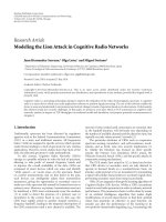
Figure 4: Belief state propagation in forward pass of Approximate
inference II. We only need to maintain the belief state the inter-
mediate distributions can be calculated based on the independence
assumptions when necessary, as indicated by the arrows within each
time slice.
Treating (x
i
, z
i
, ω
i
) as hidden state, the state transition
model can be written as
p
(
x
i
, z
i
, ω
i
| x
i−1
, z
i−1
, ω

i−1
)
= p
(
x
i
)
p
(
ω
i
)
f

z
i
| x
i−1
= k, z
(k)
i
−1
= l

.
(5)
Note that z
i
is independent of ω
i−1

given x
i−1
and z
i−1
,
and x
i
, z
i
and ω
i
are assumed to be mutually independent.
When there is no observation to be conditioned on, the prior
probability of ω
i
is determined by the topological structure
of the camera networks. So it is reasonable to assume that
the random variable ω
i
is independent of x
i
and z
i
.However,
when ω
i
is conditioned on y
0:i
,itisdependentonx
i

and z
i
through the spatiotemporal model (7). The prior probability
of object moving path p(ω
i
) can be calculated according to
the transition probabilities along that path. We use ω
(u,v)
i
=
(u, w
(r)
0
, , w
(r)
L
−1
, v) to denote the rth path of length L from
u to v,wherew
(r)
is the intermediate nodes. Then the prior
probability of object taking the rth path from u to v is
π
(r)
uv
 p

ω
(u,v)
i

= r

=
π
uw
(r)
0


L−1
l=1
π
w
(r)
l
−1
w
(r)
l

π
w
(r)
L
−1
u

r
π
uw

(r)
0


L−1
l=1
π
w
(r)
l
−1
w
(r)
l

π
w
(r)
L
−1
u
.
(6)
The spatiotemporal observation model changed to
p

d
i
, c
i

| x
i
= k, z
i
, ω
i
, y
0:i−1

=
p

d
i
| x
i
= k, z
(k)
i
= l, ω
(u,v)
i
= r, d
l
, c
l
= u, c
i
= v


×
p

c
i
= v | x
i
= k, z
(k)
i
= l, ω
(u,v)
i
= r, d
l
, c
l
= u

=
⎧
⎪
⎨
⎪
⎩
c, l = 0,
N

d
i

−d
l
; t
(r)
uv
, s
(r)
uv

, l
/
=0.
(7)
Based on the Gaussian assumption, the mean and variance
parameters in (7) can be calculated directly from the
parameter matrix A of the VSN. The mean time of the object
moving from u to v along path r is
t
(r)
uv
= t
uw
(r)
0
+
L−1

l=1
t
w

(r)
l
−1
w
(r)
l
+ t
w
(r)
L
−1
v
. (8)
The variance of travelling time of the object moving from u
to v along path r is
s
(r)
uv
= s
uw
(r)
0
+
L−1

l=1
s
w
(r)
l

−1
w
(r)
l
+ s
w
(r)
L
−1
v
. (9)
Equations (6), (8), and (9) define a composite parameter
matrix A with the same size as A.EachentryofA has
6 EURASIP Journal on Advances in Signal Processing
R
L
uv
elements, and the rth element is composed of π
(r)
uv
,
t
(r)
uv
,ands
(r)
uv
. If the Gaussian assumption does not hold,
the composite parameter matrix
A cannot be constituted

directly from A. In this case,
A should be established
manually. For example, if we assume that the traveling
time between two directly connected cameras follows the
log-normal distribution, which is useful for modeling the
object’s long stay between cameras, the total traveling time
along a specific path has no closed-form expression, but
can be reasonably approximated by another log-normal
distribution. A commonly used approximation is obtained
by matching the mean and variance [23].
The model defined by (5)–(7) can be considered as
a high-order probabilistic model in that it is capable of
describing object’s transitions between nonadjacent nodes in
the camera networks. The order of the model is determined
by the path length L.
3.4. Graphical Representation. Dynamic Bayesian networks
model probabilistic time series as a directed graph, where
the nodes represent random variables and directed edges
correspond to conditional probability distributions. Figure 2
shows the dynamic Bayesian networks model of the data
association problem in VSN.
In Figure 2 the arrows directed to z
i
are defined by (2);
the arrows directed to y
i
are defined by (3)and(7). To
complete the model, we set z
(k)
1

= 0, for k = 1, , K.
4. Exact Inference
Based on the dynamic Bayesian networks model shown in
Figure 2, data association problem in VSN can be solved
by inferring the posterior marginal distribution of labeling
variable p(x
i
| y
0:i
) from the observations and selecting the
label with the highest posterior probability. In this section
we present the exact inference algorithms, including forward
pass and backward pass, then show the intractability of the
exact inference when the number of objects is large.
4.1. Forward Pass for Exact Inference. From Figure 2 we can
see that ω
i
plays a role within a single time slice in DBN
model, thus we define the belief state as the joint posterior
probability of x
i
and z
i
and update it recursively based on
the observation y
i
at each time instance. Having the state
transition model and observation model in hand, this is a
standard state estimation problem. From Bayesian rule, the
forward pass belief state can be written as

p

x
i
, z
i
| y
0:i

=

ω
i
p

x
i
, z
i
, ω
i
| y
0:i

=
1
L
i

ω

i
p

y
i
| x
i
, z
i
, ω
i
, y
0:i−1

p

x
i
, z
i
, ω
i
| y
0:i−1

=
1
L
i
λ

i
(
x
i
= k
)
η
i

z
(k)
i
= l

p

z
i
| y
0:i−1

,
(10)
where L
i
= p(y
i
| y
0:i−1
) is the normalizing constant. The

appearance and spatiotemporal information are injected into
the model through the terms λ
i
and η
i
,respectively,whichare
defined as follows:
λ
i
(
x
i
= k
)
= p
(
x
i
= k
)
p
(
o
i
| x
i
= k
)
for k = 1, ,K,
η

i

z
(k)
i
= l

=

ω
(u,v)
i
p

ω
(u,v)
i

×
p

d
i
| x
i
= k, z
(k)
i
= l, ω
(u,v)

i
,
d
l
, c
l
= u, c
i
= v

for l = 0, , i −1.
(11)
Note that the probability items corresponding to all elements
in ω
i
except ω
(u,v)
i
are summed to one and ω
(u,v)
i
is completely
encapsulated in the term η
i
.Itturnsoutatthispointthat
introducing ω
i
results in a mixed spatiotemporal observation
model, as it can be expressed in terms of a weighted sum of
probabilities conditioned on different paths. To calculate the

predictive probability of z
i
, we first calculate the predictive
probability of the joint state (z
i
, x
i−1
) and then marginalize
x
i−1
out. It can be written as
p

z
i
, x
i−1
= j | y
0:i−1

=

z
i−1
f
(
z
i
| x
i−1

, z
i−1
)
p

x
i−1
= j, z
i−1
| y
0:i−1

=
⎧
⎪
⎪
⎪
⎪
⎪
⎪
⎪
⎪
⎪
⎪
⎪
⎪
⎪
⎨
⎪
⎪

⎪
⎪
⎪
⎪
⎪
⎪
⎪
⎪
⎪
⎪
⎪
⎩
i−2

m=0
p

x
i−1
= j, z
(j)
i
−1
= m, z
(¬j)
i
−1
= z
(¬j)
i

| y
0:i−1

if z
(j)
i
= i −1, z
(¬j)
i
= 0, , i −2,
otherwise
0,
(12)
where z
(¬j)
i
 z
(1:K)
i
\z
(j)
i
. From the deterministic relationship
of (2), if x
i−1
= j, the summands in the first line of (12)are
nonzero only when z
(¬j)
i
−1

= z
(¬j)
i
. The last line of (12)ensures
that all z
(k)
i
cannot be less than i −1 simultaneously and only
z
(j)
i
can be equal to i − 1ifx
i−1
= j.
4.2. Backward Pass for Exact Inference. In backward infer-
ence, future observations can be used to further modify the
estimation of current state. Following the similar manner of
derivation in [24], and exploiting the conditional indepen-
dency encoded in the DBN model shown in Figure 2, the
backward belief state can be written as
EURASIP Journal on Advances in Signal Processing 7
p

x
i
, z
i
| y
0:N


=

x
i+1

z
i+1
p

x
i
, z
i
, x
i+1
, z
i+1
| y
0:N

=

x
i+1

z
i+1
p

x

i
, z
i
| x
i+1
, z
i+1
, y
0:i+1

p

x
i+1
, z
i+1
| y
0:N

p

y
0:N

p

y
0:N

=


x
i+1

z
i+1
p

y
i+1
| x
i+1
, z
i+1
, y
0:i

p
(
x
i+1
, z
i+1
| x
i
, z
i
)
p


x
i
, z
i
| y
0:i

p

y
0:i

p

x
i+1
, z
i+1
| y
0:i+1

p

y
0:i+1

p

x
i+1

, z
i+1
| y
0:N

=
1
L
i+1
p

x
i
, z
i
| y
0:i


x
i+1

z
i+1
λ
i+1
(
x
i+1
= k

)
η
i+1

z
(k)
i+1
= l

f
(
z
i+1
| x
i
, z
i
)
p

x
i+1
, z
i+1
| y
0:N

p

x

i+1
, z
i+1
| y
0:i+1

=
1
L
i+1
p

x
i
, z
i
| y
0:i


x
i+1
λ
i+1
(
x
i+1
= k
)
η

i+1

z
(k)
i+1

x
i
, z
(k)
i

p

x
i+1
, z
i+1
(
x
i
, z
i
)
| y
0:N

p

x

i+1
, z
i+1
(
x
i
, z
i
)
| y
0:i+1

.
(13)
Note that the normalizing constant in (13)isalready
available and
z
(k)
i+1
is a function of x
i
and z
(k)
i
,whichisdefined
by (2).
Although the deterministic relation in (2) has simplified
the inference computation significantly, it is clear in (10)and
(13) that maintaining both forward and backward belief state
is still intractable as the joint state space is the Cartesian

product of the state space of x
i
and K spaces of all z
(k)
i
.
At step i of forward passing, for example, there are Ki
K
elements which need to be evaluated for updating the belief
state. To make the inference practicable, we have to resort to
approximate inference.
5. Approximate Inference
The basic idea of approximate inference is factorization.
By factorizing the joint belief state into the product of
several distributions of smaller sets of random variables,
the memory and computational resources required for
storing and updating belief state can be reduced. Inevitably,
this factorization will introduce errors in belief state rep-
resentation if the random variables in different sets are
not indeed independent. However, Boyen and Koller [17]
showed that, in terms of the Kullback-Leibler divergence, the
inference error introduced by factorized representation of the
belief state of discrete stochastic process is not accumulated
infinitely over time. Furthermore, if the factorization is
tailored to the specific structure of the process, the error
has a bound determined by the minimum mixing rate of
the involved subprocesses and the interaction among them.
Theoretical results in [25] showed that using conditional
independent clusters for approximate representation yields
tighter bound. Although the theoretical results have not been

extended to general stochastic process including continuous
variables and to the case of reasoning backward in time,
it is clearly suggested that for approximate inference, the
structure of DBN may be exploited for computational gain
in these circumstances. Following this line, in this section
we present two kinds of factorization schemes based on
the structure of DBN shown in Figure 2 and provide the
corresponding forward and backward algorithms. The effect
of the algorithms is shown in Section 7 with simulations and
experiments.
The intractability of exact inference of our problem
comes from the interdependency between variables. “Active
path” [26] is a convenient tool for analyzing the dependence
structure in belief networks: an active path from node i
to j given node set K is a simple trail between i and j,
such that every node with two incoming arcs on the trail
is or has a descendant in K and every other node on the
trail is not functionally determined by K.Twonodesare
interdependent if they are connected by an active path. In
Figure 2 we can identify the following two kinds of active
paths: (a) active paths within a single time slice, z
(j)
i
and z
(k)
i
are coupled through the path z
(j)
i
− y

i
− z
(k)
i
,andx
i
and z
(k)
i
are coupled through x
i
− y
i
−z
(k)
i
; (b) active paths across the
past time slices, and z
(j)
i
and z
(k)
i
are coupled through the
paths z
(j)
i
− x
i−1
− z

(k)
i
and z
(j)
i
− z
(j)
i
−1
− y
i−1
− z
(k)
i
−1
− z
(k)
i
,
and the longer paths z
(j)
i
− z
(j)
i
−1
− x
i−2
− z
(k)

i
−1
− z
(k)
i
and
z
(j)
i
−z
(j)
i
−1
−z
(j)
i
−2
−y
i−2
−z
(k)
i
−2
−z
(k)
i
−1
−z
(k)
i

, and so on. It should
be noticed, however, that the active paths between z
(k)
i
scan
be disconnected if the value of x at proper time slice is given.
For example, z
(j)
i
− y
i
− z
(k)
i
breaks if x
i
is given; the pair of
paths z
(j)
i
−x
i−1
−z
(k)
i
and z
(j)
i
−z
(j)

i
−1
−y
i−1
−z
(k)
i
−1
−z
(k)
i
break
if x
i−1
is given, and so on.
In Section 5.1, we present a simple approximate inference
approach based on the marginal independence assumption
which naively neglects all the active paths mentioned above.
In Section 5.2 we propose another approximate inference
which neglects the active paths across the past time slices and
preserves the path within the current time slice and factorizes
the joint belief state based on the assumed conditional
independence. In simulations the second approximate infer-
ence demonstrates better compromise between inference
accuracy and computational efficiency. In Section 5.3 we
discuss the problem of choice of active path for approximate
inference in more detail and the relationship with other
works.
8 EURASIP Journal on Advances in Signal Processing
5.1. Approximate Inference I. In the first factorization

scheme, the joint belief state is naively decomposed into the
product of marginal distributions of x
i
and z
(k)
i
, that is,
p

x
i
, z
i
| y
0:i

≈

p

x
i
, z
i
| y
0:i

=

p


x
i
| y
0:i

K

k=1

p

z
(k)
i
| y
0:i

,
p

x
i
, z
i
| y
0:N

≈


p

x
i
, z
i
| y
0:N

=

p

x
i
| y
0:N

K

k=1

p

z
(k)
i
| y
0:N


.
(14)
At step i in the forward pass, the approximate belief state

p(x
i−1
, z
i−1
| y
0:i−1
) is propagated through the transition
model, obtaining

p(x
i
, z
i
| y
0:i−1
), and conditioned on
the current observation, obtaining

p(x
i
, z
i
| y
0:i
), then
approximated by (14), obtaining


p(x
i
, z
i
| y
0:i
). The process
of backward pass is similar.
5.1.1. Forward Pass in Approximate Inference I. To d e r i v e
the forward pass algorithm, we first calculate the marginal
distributions

p
i
in (14)from(10) and then try to express
them in terms of the marginal distributions of the last time
instance

p
i−1
based on the independence assumption. The
marginal distribution of x
i
is

p

x
i

= k | y
0:i

=

z
i

p

x
i
= k, z
i
| y
0:i

=
1
L
f
i
λ
i
(
x
i
= k
)


z
i
η
i

z
(k)
i
= l


p

z
i
| y
0:i−1

=
1
L
f
i
λ
i
(
x
i
= k
)


z
(k)
i
η
i

z
(k)
i
= l


p

z
(k)
i
= l | y
0:i−1

.
(15)
For k = 1, , K, the marginal distribution of z
(k)
i
is

p


z
(k)
i
= l | y
0:i

=

x
i

z
(¬k)
i

p

x
i
, z
i
| y
0:i

=
1
L
f
i


x
i

z
(¬k)
i
λ
i
(
x
i
= k
)
η
i

z
(k)
i
= l


p

z
i
| y
0:i−1

=

1
L
f
i
λ
i
(
x
i
= k
)
η
i

z
(k)
i
= l


p

z
(k)
i
= l | y
0:i−1

+
1

L
f
i
K

x
i
= 1
x
i
/
=k
λ
i

x
i
= j


z
(j)
i
η
i

z
(j)
i
= m


×

p

z
(j)
i
= m, z
(k)
i
= l | y
0:i−1

.
(16)
There are two kinds of predictive distributions in (15)and
(16), one is over single z
(k)
i
, and the other is over the pair
(z
(j)
i
, z
(k)
i
). We first calculate the joint predictive probabilities
of them with x
i−1

, then marginalize x
i−1
out. The joint
predictive distribution of (z
(k)
i
, x
i−1
)is

p

z
(k)
i
= l, x
i−1
= n | y
0:i−1

=

z
(k)
i
−1
f

z
(k)

i
= l | x
i−1
= n, z
(k)
i
−1


p

x
i−1
= n, z
(k)
i
−1
| y
0:i−1

=
⎧
⎪
⎪
⎪
⎪
⎪
⎪
⎪
⎪

⎨
⎪
⎪
⎪
⎪
⎪
⎪
⎪
⎪
⎩

p

x
i−1
= k | y
0:i−1

if n = k, l = i −1,

p

x
i−1
= n | y
0:i−1

×

p


z
(k)
i
−1
= l | y
0:i−1

if n
/
=k, l = 0:i −2,
otherwise 0.
(17)
The joint predictive distribution of (z
(k)
i
, z
(j)
i
, x
i−1
)is

p

z
(j)
i
= m, z
(k)

i
= l, x
i−1
= n | y
0:i−1

=

z
(j)
i
−1

z
(k)
i
−1
f

z
(j)
i
= m, z
(k)
i
= l | x
i−1
= n, z
(j)
i

−1
, z
(k)
i
−1

×

p

x
i−1
= n, z
(j)
i
−1
, z
(k)
i
−1
| y
0:i−1

=
⎧
⎪
⎪
⎪
⎪
⎪

⎪
⎪
⎪
⎪
⎪
⎪
⎪
⎪
⎪
⎪
⎪
⎪
⎪
⎪
⎪
⎪
⎪
⎪
⎪
⎪
⎪
⎪
⎪
⎪
⎪
⎪
⎪
⎪
⎨
⎪

⎪
⎪
⎪
⎪
⎪
⎪
⎪
⎪
⎪
⎪
⎪
⎪
⎪
⎪
⎪
⎪
⎪
⎪
⎪
⎪
⎪
⎪
⎪
⎪
⎪
⎪
⎪
⎪
⎪
⎪

⎪
⎪
⎩

p

x
i−1
= j | y
0:i−1


p

z
(k)
i
−1
= l | y
0:i−1

if n = j, m = i −1, l = 0:i − 2,

p

x
i−1
= k | y
0:i−1



p

z
(j)
i
−1
= m | y
0:i−1

if n = k, m = 0:i −2, l = i −1,

p

x
i−1
= n | y
0:i−1


p

z
(j)
i
−1
= m | y
0:i−1

×


p

z
(k)
i
−1
= l | y
0:i−1

if n
/
= j, n
/
=k, m = 0:i − 2, l = 0:i −2,
otherwise
0.
(18)
Note that the independence assumption in (14) plays its
role in the last line of (17)and(18). To update the
belief state at step i using (15)–(18), we only need to
evaluate the probabilities of K + Ki different configurations.
The computation is greatly simplified. The forward pass
algorithm for approximate inference I is depicted graphically
in Figure 3.
EURASIP Journal on Advances in Signal Processing 9
5.1.2. Backward Pass in Approximate Inference I. The deriva-
tion of backward pass algorithm is straightforward. We first
substitute (14) into (13), obtaining


p

x
i
, z
i
| y
0:N

=
1
L
b
i+1

p

x
i
, z
i
| y
0:i

×

x
i+1
λ
i+1

(
x
i+1
= k
)
η
i+1

z
(k)
i+1

x
i
, z
(k)
i

×

p

x
i+1
, z
i+1
(
x
i
, z

i
)
| y
0:N


p

x
i+1
, z
i+1
(
x
i
, z
i
)
| y
0:i+1

=
1
L
b
i+1

p

x

i
| y
0:i


τ

p

z
(τ)
i
| y
0:i

·

x
i+1
λ
i+1
(
x
i+1
= k
)
η
i+1

z

(k)
i+1

x
i
, z
(k)
i

×

p

x
i+1
| y
0:N


p

x
i+1
| y
0:i+1


τ

p


z
(τ)
i+1

x
i
, z
(τ)
i

|
y
0:N


p

z
(τ)
i+1

x
i
, z
(τ)
i

|
y

0:i+1

.
(19)
Note that in approximate inference the normalization con-
stant L
b
i+1
/
=L
f
i+1
. Then we calculate the marginal distribution
of x
i

p

x
i
= n | y
0:N

=

z
i

p


x
i
, z
i
| y
0:N

=
1
L
b
i+1

p

x
i
= n | y
0:i

×

x
i+1
λ
i+1
(
x
i+1
= k

)

τ

z
(τ)
i
η
(k)
i+1

x
i
, z
(τ)
i

φ
i+1

x
i
, z
(τ)
i

(20)
and the marginal distribution of z
(k)
i


p

z
(j)
i
= m | y
0:N

=

x
i

z
(¬j)
i

p

x
i
, z
i
| y
0:N

=
1
L

b
i+1

x
i+1
λ
i+1
(
x
i+1
= k
)
·

x
i

p

x
i
| y
0:i

η
(k)
i+1

x
i

, z
(j)
i
= m

φ
i+1

x
i
, z
(j)
i
= m

×

τ
/
= j

z
(τ)
i
η
(k)
i+1

x
i

, z
(τ)
i

φ
i+1

x
i
, z
(τ)
i

,
(21)
p(x
i
= k|y
0:N
)
Inference
Parameter
estimation
(α
h
, μ
k
, σ
k
)

Figure 5: The EM framework. The inference module is imple-
mented with the algorithms presented in Sections 4 and 5, and the
parameter estimation module is implemented with (34)–(36).
where the terms λ
i+1
, η
(k)
i+1
,andφ
i+1
are defined as
λ
i+1
(
x
i+1
= k
)
= λ
i+1
(
x
i+1
= k
)

p

x
i+1

| y
0:N


p

x
i+1
| y
0:i+1

, (22)
η
(k)
i+1

x
i
= n, z
(τ)
i
= l

=
⎧
⎪
⎪
⎪
⎪
⎨

⎪
⎪
⎪
⎪
⎩
1ifτ
/
=k,
η
i+1

z
(k)
i+1
= i

if τ = k, n = k,
η
i+1

z
(k)
i+1
= l

if τ = k, n
/
=k,
(23)
φ

i+1

x
i
= n, z
(τ)
i
= l

=
⎧
⎪
⎪
⎪
⎪
⎪
⎪
⎪
⎪
⎨
⎪
⎪
⎪
⎪
⎪
⎪
⎪
⎪
⎩


p

z
(τ)
i+1
= i | y
0:N


p

z
(τ)
i+1
= i | y
0:i+1


p

z
(τ)
i
= l | y
0:i

if n = τ,

p


z
(τ)
i+1
= l | y
0:N


p

z
(τ)
i+1
= l | y
0:i+1


p

z
(τ)
i
= l | y
0:i

if n
/
=τ.
(24)
5.2. Approximate Inference II. In the second factorization
scheme, we preserve the interdependence between x

i
and z
i
and assume that z
(j)
i
and z
(k)
i
are conditional independent
given x
i
. Then the joint belief state is decomposed as
p

x
i
, z
i
| y
0:i

≈

p


x
i
, z

i
| y
0:i

=

p


x
i
| y
0:i

K

k=1

p


z
(k)
i
| x
i
, y
0:i

,

p

x
i
, z
i
| y
0:N

≈

p


x
i
, z
i
| y
0:N

=

p


x
i
| y
0:N


K

k=1

p


z
(k)
i
| x
i
, y
0:N

.
(25)
The process of forward and backward pass is the same as
before, except for the approximation manner of the belief
state.
5.2.1. Forward Pass in Approximate Inference II. To w r i te
down the forward pass algorithm for belief state representa-
tion in (25), we need to compute the marginal distributions

p

over x
i
and (x

i
, z
(k)
i
). The former can be calculated as in
10 EURASIP Journal on Advances in Signal Processing
(15),butwithdifferent definition of

p

(z
(k)
i
| y
0:i−1
). The
latter can be written as

p


x
i
= j, z
(k)
i
= l | y
0:i

=


z
(¬k)
i

p


x
i
= j, z
(k)
i
= l, z
(¬k)
i
| y
0:i

=
1
L
f
i
λ
i

x
i
= j



z
(¬k)
i
η
i

z
(j)
i
= m


p


z
i
| y
0:i−1

=
⎧
⎪
⎪
⎪
⎪
⎪
⎪

⎪
⎪
⎪
⎪
⎪
⎪
⎨
⎪
⎪
⎪
⎪
⎪
⎪
⎪
⎪
⎪
⎪
⎪
⎪
⎩
1
L
f
i
λ
i
(
x
i
= k

)
η
i

z
(k)
i
= l

×

p


z
(k)
i
= l | y
0:i−1

if j = k,
1
L
f
i
λ
i

x
i

= j


z
(j)
i
η
i

z
(j)
i
= m

×

p


z
(j)
i
= m, z
(k)
i
= l | y
0:i−1

if j
/

=k.
(26)
Based on the independence assumption in (25), the two
predictive distributions in (17)and(18) are redefined as

p


z
(k)
i
= l, x
i−1
= n | y
0:i−1

=

z
(k)
i
−1
f

z
(k)
i
= l | x
i−1
= n, z

(k)
i
−1


p


x
i−1
= n, z
(k)
i
−1
| y
0:i−1

=
⎧
⎪
⎪
⎪
⎪
⎨
⎪
⎪
⎪
⎪
⎩


p


x
i−1
= k | y
0:i−1

if n = k, l = i −1,

p


x
i−1
= n, z
(k)
i
−1
= l | y
0:i−1

if n
/
=k, l = 0:i −2,
otherwise 0,
(27)

p



z
(j)
i
= m, z
(k)
i
= l, x
i−1
= n | y
0:i−1

=

z
(j)
i
−1

z
(k)
i
−1
f

z
(j)
i
= m, z
(k)

i
= l | x
i−1
= n, z
(j)
i
−1
, z
(k)
i
−1

×

p


x
i−1
= n, z
(j)
i
−1
, z
(k)
i
−1
| y
0:i−1


=
⎧
⎪
⎪
⎪
⎪
⎪
⎪
⎪
⎪
⎪
⎪
⎪
⎪
⎪
⎪
⎪
⎪
⎪
⎪
⎪
⎪
⎪
⎪
⎪
⎪
⎪
⎪
⎪
⎪

⎪
⎪
⎪
⎨
⎪
⎪
⎪
⎪
⎪
⎪
⎪
⎪
⎪
⎪
⎪
⎪
⎪
⎪
⎪
⎪
⎪
⎪
⎪
⎪
⎪
⎪
⎪
⎪
⎪
⎪

⎪
⎪
⎪
⎪
⎪
⎩

p


x
i−1
= j, z
(k)
i
−1
= l | y
0:i−1

if n = j, m = i −1, l = 0:i − 2,

p


x
i−1
= k, z
(j)
i
−1

= m | y
0:i−1

if n = k, m = 0:i −2, l = i −1,

p


z
(j)
i
−1
= m, x
i−1
= n | y
0:i−1


p


p


x
i−1
= n | y
0:i−1

×


z
(k)
i
−1
= l, x
i−1
= n | y
0:i−1

if n
/
= j, n
/
=k, m = 0:i − 2, l = 0:i − 2,
otherwise
0.
(28)
When belief state is updated by (26)–(28)atstepi, K +
K
2
i elements need to be evaluated. The forward pass
algorithm for approximate inference II is depicted graphically
in Figure 4. Although the computational burden increases to
some extent compared with approximation inference I (but
still much less than that in exact algorithm), simulation
results show that the inference accuracy is improved signif-
icantly, approaching that of the exact algorithm.
5.2.2. Backward Pass in Approximate Inference II. As before,
to derive the backward pass algorithm for approximate

inference II,wesubstitute(25) into (13), obtaining

p


x
i
, z
i
| y
0:N

=
1
L
b
i+1

p


x
i
| y
0:i


τ

p



z
(τ)
i
| x
i
, y
0:i

·

x
i+1
λ
i+1
(
x
i+1
= k
)
η
i+1

z
(k)
i+1

x
i

, z
(k)
i


p


x
i+1
| y
0:N


p


x
i+1
| y
0:i+1

×

τ

p


z

(τ)
i+1

x
i
, z
(τ)
i

|
x
i+1
, y
0:N


p


z
(τ)
i+1

x
i
, z
(τ)
i

|

x
i+1
, y
0:i+1

,
(29)
then calculate the marginal distribution of x
i

p


x
i
= n | y
0:N

=

z
i

p


x
i
, z
i

| y
0:N

=
1
L
b
i+1

p


x
i
= n | y
0:i


x
i+1
λ
i+1
(
x
i+1
= k
)
×

τ


z
(τ)
i
η
(k)
i+1

x
i
, z
(τ)
i

ψ
i+1

x
i
, z
(τ)
i
, x
i+1

(30)
and the marginal distribution of (x
i
, z
(k)

i
)

p


x
i
= n, z
(j)
i
= m | y
0:N

=

z
(¬j)
i

p


x
i
, z
i
| y
0:N


=
1
L
b
i+1

x
i+1
λ
i+1
(
x
i+1
= k
)
η
(k)
i+1

x
i
, z
(j)
i

ψ
i+1

x
i

, z
(j)
i
, x
i+1

×

τ
/
= j

z
(τ)
i
η
(k)
i+1

x
i
, z
(τ)
i

ψ
i+1

x
i

, z
(τ)
i
, x
i+1

,
(31)
EURASIP Journal on Advances in Signal Processing 11
where
λ
i+1
,andη
(k)
i+1
are defined by (22)and(23). ψ
i+1
is
defined as
ψ
i+1

x
i
= n, z
(τ)
i
= l, x
i+1
= k


=
⎧
⎪
⎪
⎪
⎪
⎪
⎪
⎪
⎪
⎪
⎪
⎪
⎪
⎪
⎪
⎪
⎪
⎪
⎪
⎪
⎪
⎪
⎪
⎪
⎪
⎪
⎪
⎪

⎪
⎪
⎪
⎪
⎪
⎪
⎪
⎪
⎪
⎪
⎨
⎪
⎪
⎪
⎪
⎪
⎪
⎪
⎪
⎪
⎪
⎪
⎪
⎪
⎪
⎪
⎪
⎪
⎪
⎪

⎪
⎪
⎪
⎪
⎪
⎪
⎪
⎪
⎪
⎪
⎪
⎪
⎪
⎪
⎪
⎪
⎪
⎪
⎩

p


z
(τ)
i+1
= i, x
i+1
= k | y
0:N



p


z
(τ)
i+1
= i, x
i+1
= k | y
0:i+1

·

p


x
i+1
= k | y
0:i+1


p


x
i+1
= k | y

0:N

·

p


z
(τ)
i
= l, x
i
= n | y
0:i


p


x
i
= n | y
0:i

if n = τ,

p


z

(τ)
i+1
= l, x
i+1
= k | y
0:N


p


z
(τ)
i+1
= l, x
i+1
= k | y
0:i+1

·

p


x
i+1
= k | y
0:i+1



p


x
i+1
= k | y
0:N

·

p


z
(τ)
i
= l, x
i
= n | y
0:i


p


x
i
= n | y
0:i


,ifn
/
=τ.
(32)
5.3. Discussion. In this section we will discuss the problem
of choosing active path for approximate inference in more
detail. Here we define the belief state as the joint distribution
of (z
1:K
i
, x
1:i
) and the exact forward inference can be reformu-
lated as
p

z
1:K
i
, x
1:i
| y
0:i

=
1
L
i
λ
i

(
x
i
= k
)
η
i

z
(k)
i
= l

×
p

z
1:K
i
| x
1:i−1

p

x
1:i−1
| y
0:i−1

=

1
L
i
λ
i
(
x
i
= k
)
η
i

z
(k)
i
= l

×
K

j=1
p

z
(j)
i
| x
1:i−1


p

x
1:i−1
| y
0:i−1

,
(33)
where λ
i
and η
i
are defined in (11). Note that the joint
predictive distribution of z
1:K
i
is completely decomposable
given x
1:i−1
. In exact inference using (33), we have to
enumerate in the sampling space of x
1:i−1
. This just shifts the
problem from the intractable enumeration of z
1:K
i
to that of
x
1:i−1

. For tractable inference, we must discard some of the
conditioning variables x
1:i−1
. Discarding all x
1:i−1
leads to the
proposed approximate inference II.
Formulation (33)providesaclearerviewofthe“relative
significance” of active path corresponding to variable x
τ
,
τ
= 1:i − 1. Note that with some probability δ
τ
, z
(j)
i
is functionally determined by x
τ
. In other words, the τth
active path is disconnected by x
τ
with probability δ
τ
.Thus
we can use δ
τ
as a measure of the “relative significance”
of the τth active paths. It is easy to show that δ
τ

decreases
exponentially as τ varying from i
− 1to1.Infact,for
time slice i, the relative significance of i
− 1th path is
0 5 10 15 20 25 30 35 40
0
2
4
(a)
0 5 10 15 20 25 30 35 40
0
2
4
(b)
0 5 10 15 20 25 30 35 40
0
2
4
(c)
0 5 10 15 20 25 30 35 40
0
2
4
(d)
Figure 6: Marginal distribution of labeling variable in exact
inference. The 24th and 34th observations are missed, depicted
as dashed column. The true labels are depicted by stars. Each
column represents the marginal distribution of the label of an
observation. Grayscale corresponds to probability value. Black

represents probability 1 and white probability 0. (a) Forward pass
with 0-order model. (b) Forward pass with 1-order model. (c)
Backward pass with 0-order model. (d) Backward pass with 1-order
model.
δ
i−1
= p(x
i−1
= j), and the relative significance of i − 2th
path is δ
i−2
= p(x
i−1
/
= j)p(x
i−2
= j), and so on (we omit the
conditioning variables y
0:i−1
temporally for clarity). This fact
implies that the “recent” active paths are far more important
than the “ancient” ones for accurate inference as they are
less likely to be disconnected. We delete the conditioning
variables x
τ
in (33)onebyonefromτ = 1toi−1, resulting in
a set of approximate inference algorithms and compare them
with the proposed approximate inference II. We observed in
simulations that the conditioning variables x
τ

earlier than
i
− 1havemuchlesseffect on inference accuracy than x
i−1
and including x
i−1
can only improve the inference accuracy
to a limited extent, but at the cost of a significant increase in
computational burden.
It is interesting to relate our works with [27], where
an approximate variational inference approach is proposed
based on conditional entropy decomposition. As evaluating
the negative entropy term in the objective function of
the optimization problem is intractable if the graph size
is large, and the authors decompose the full model into
a sum of conditional entropies using the entropy chain
rule, and then restrict the number of conditioning variables
by discarding some of them. Since removing conditioning
variables cannot decrease the entropy, this approximation
leads to an upper bound of the objective function. In
fact, in [27] the approximation of inference manifests in
replacing the joint distribution of interest with a product
of conditional distributions and discarding some of the
conditioning variables based on the assumed conditional
12 EURASIP Journal on Advances in Signal Processing
0 5 10 15 20 25 30 35 40
0
2
4
(a)

0 5 10 15 20 25 30 35 40
0
2
4
(b)
0 5 10 15 20 25 30 35 40
0
2
4
(c)
0 5 10 15 20 25 30 35 40
0
2
4
(d)
0 5 10 15 20 25 30 35 40
0
2
4
(e)
0 5 10 15 20 25 30 35 40
0
2
4
(f)
Figure 7: Marginal distribution of labeling variable in exact inference. The 3rd, 8th, 13th, 28th, 32nd, and 33rd observations are missed,
depicted as dashed column. The true labels are depicted by stars. Each column represents the marginal distribution of the label of an
observation. Grayscale corresponds to probability value. Blacks represent probability 1 and white probability 0. (a) Forward pass with 0-
order model. (b) Forward pass with 1-order model. (c) Forward pass with 2-order model. (d) Backward pass with 0-order model. (e)
Backward pass with 1-order model. (f) Backward pass with 2-order model.

independence, which is just the same scheme used in our
approximate inference II. The authors in [27] point out that
the more conditioning variables preserved, the tighter the
bound is. This is also consistent with our results. However, it
is not clear in [27] how to choose the conditioning variables
in an optimal way. Besides, our approximate inference (I
and II) is similar with the Factored Frontier algorithm [28]
in that both of them factorize the joint belief state. But
there is one important difference: our algorithms update
the factored belief state from time t
− 1tot exactly
before computing the marginals in t,whereasFactored
Frontier computes the approximate marginals directly based
on additional independence assumption, resulting in more
errors in calculation.
It is tempting in application that the independence
structure can be discovered automatically. This enables the
algorithm to choose the approximation scheme adaptively
according to changing situations. We notice that in [29]an
incremental thin junction tree algorithm is proposed which
can adaptively choose a set of clusters and separators, that is,
a junction tree, at each time step to approximate the belief
state. We plan to incorporate this idea into our method in
the future.
6. EM Framework for Unknown
Appearance Parameters
In the previous discussion, we assumed that the appearance
models of the objects under tracking are available. However,
in typical scenarios of practical interests, the parameters
of the appearance model are usually unknown and need

to be estimated from observations. If we had known the
label of each observation, that is, the object from which
the observation is generated, the parameter estimation is
straightforward. But the labels are also unknown and need to
be estimated with data association algorithms. Considering
the hidden labels as missing data, the problems of parameter
estimation and data association can be solved simultaneously
under the EM framework [30].
In this paper, the appearance observations are assumed
to be generated from Gaussian mixture model, and the E-
step and M-step in the EM framework take a very intuitive
and simple form. We use Θ
={α
k
, μ
k
, σ
k
}
K
k
=1
to denote
the model parameters, where α
k
 p(x
i
= k) is the
prior probability of the label k, μ
k

and σ
k
are mean and
variance of appearance of object k. In E-step, based on
the old guess of the model parameters Θ
old
,wecalculate
the ownership probability of each observation, that is, the
posterior probability of the hidden label corresponding to
each observation, p(x
i
|y
0:N
, Θ
old
), with the data association
algorithm presented in previous sections. Note that if we
use forward passing algorithm for inference, the ownership
probability is p(x
i
|y
0:i
, Θ
old
). In M-step, the model param-
eters are updated as in classical EM algorithm for Gaussian
mixture model [31]
α
new
k

=
1
N
N

i=1
p

x
i
= k | y
0:N
, Θ
old

,
μ
new
k
=

N
i
=1
o
i
p

x
i

= k | y
0:N
, Θ
old


N
i
=1
p

x
i
= k | y
0:N
, Θ
old

,
σ
new
k
=

N
i=1
p

x
i

= k | y
0:N
, Θ
old


o
i
−μ
new
k

o
i
−μ
new
k



N
i=1
p

x
i
= k | y
0:N
, Θ
old


.
(34)
The EM framework presented above is shown in Figure 5.
It can be thought of as a generalization of the classical
EM algorithm for the GMM [31] in that it calculates the
ownership probabilities with inference algorithms based on
both appearance and spatiotemporal information, instead
of calculating them with Bayes rule based solely on the
current appearance observation. Note that the EM proposed
above can only work in an offline manner. Yet the learnt
EURASIP Journal on Advances in Signal Processing 13
0 100 200 300 400 500 600 700 800 900 1000
fwd approximate I
0
1
2
3
4
5
6
(a)
0 100 200 300 400 500 600 700 800 900 1000
bwd approximate I
0
2
4
6
8
10

12
(b)
0 100 200 300 400 500 600 700 800 900 1000
fwd approximate II
0
0.2
0.4
0.6
0.8
1
1.2
1.4
(c)
0 100 200 300 400 500 600 700 800 900 1000
bwd approximate II
0
0.5
1
1.5
2
2.5
(d)
0 100 200 300 400 500 600 700 800 900 1000
fwd
10
−20
10
−15
10
−10

10
−5
10
0
10
5
Approximate I
Approximate II
(e)
0 100 200 300 400 500 600 700 800 900 1000
bwd
10
−16
10
−14
10
−12
10
−10
10
−8
10
−6
10
−4
10
−2
10
0
10

2
Approximate I
Approximate II
(f)
Figure 8: KL divergence caused by approximate inference. (a) Forward approximate I. (b) Backward approximate I. (c) Forward approximate
II. (d) Backward approximate II. (e) Comparison between smoothed KL divergence of forward approximates I and II in log domain. (f)
Comparison between smoothed KL divergence of backward approximates I and II in log domain.
model can be used for online data association using forward
inference algorithms. In the future, we plan to investigate
how to incorporate the inference engine into online EM
such that both model learning and data association can be
accomplished simultaneously on the fly. It is interested if we
could estimate the parameters in the spatiotemporal model
using EM as well. However, in M step, it is difficult to find
an algorithm similar to (34) to update the guessed value of
spatiotemporal parameters due to the existence of missing
detections.
7. Results
7.1. Simulations
7.1.1. Data. To generate simulation data, we use the VSN
with topological model shown as Figure 1 and specify the
parameter matrix A of VSN and the appearance model
parameters (μ
k
, σ
2
k
) of each object under tracking. The
mean travel time t
uv

between adjacent nodes u and v is
proportional to their distance, as shown in Ta b le 1 .And
14 EURASIP Journal on Advances in Signal Processing
00.511.522.53
fwd exact
Appearance noise
fwd approximate I
fwd approximate II
60
65
70
75
Matching accuracy (%)
80
85
90
95
100
(a)
00.511.522.53
bwd exact
Appearance noise
bwd approximate I
bwd approximate II
30
40
50
60
Matching accuracy (%)
70

80
90
100
(b)
Figure 9: Mean accuracy under different appearance noise level. X-axis corresponds to the variance of appearance observations. (a) Forward
inference. (b) Backward inference.
0.10.20.30.40.50.60.7
fwd exact
Traveling time noise
fwd approximate I
fwd approximate II
0
20
40
Matching accuracy (%)
60
80
100
(a)
0.10.20.30.40.50.60.7
bwd exact
Traveling time noise
bwd approximate I
bwd approximate II
0
20
40
Matching accuracy (%)
60
80

100
(b)
Figure 10: Mean accuracy under different level of traveling time standard deviation. X-axis corresponds to the ratio of standard deviation
to mean value of the traveling time observations. (a) Forward inference. (b) Backward inference.
the standard deviation of travel time is assumed to be
proportional to its mean value. In each simulation, for
the kth object, we choose its starting node randomly in
Figure 1, then generate its moving trajectory according to
the transition probabilities π
uv
. On each node along the
trajectory of the kth object, the spatiotemporal observations
d
i
and appearance observations o
i
are drawn from the
assumed Gaussian model. We assume that at each time
instance, there is only one object being observed by a camera.
Theobservationsofallobjectsarecollectedtogetherand
reordered according to the time observation, resulting in the
data set
{y
i
}.
7.1.2. Evaluation Criteria. The criterion we use is the data
association accuracy,denotedasq:
q
=
1

K
K

k=1
q
k
q
k
=



Y
k
∩Y
k



|Y
k
|
·
100%, (35)
where K is the number of objects of interest and
|·|indicates
the number of elements in a set. The term
Y
k
indicates

the “ground truth” set of observations of object k,andY
k
is the set of observations of object k determined by the
data association algorithms. To evaluate the complexity of
EURASIP Journal on Advances in Signal Processing 15
0 5 10 15 20 25 30 35 40
0
2
4
(a)
0 5 10 15 20 25 30 35 40
0
2
4
(b)
0 5 10 15 20 25 30 35 40
0
2
4
(c)
0 5 10 15 20 25 30 35 40
0
2
4
(d)
0 5 10 15 20 25 30 35 40
0
2
4
(e)

0 5 10 15 20 25 30 35 40
0
2
4
(f)
Figure 11: Marginal distribution of labeling variable in inference
with 1-order spatiotemporal model. The 3rd, 10th, 23rd, and
25th observations are missed, depicted as dashed column. The
true labels are depicted by stars. Each column represents the
marginal distribution of the label of an observation. Grayscale
corresponds to probability value. Black represents probability 1, and
white probability 0. (a) Forward exact. (b) Forward approximate
I. (c) Forward approximate II. (d) Backward exact. (e) Backward
approximate I. (f) Backward approximate II.
Table 1: The mean travel time between adjacent nodes.
abcdefghi j
a0588085000000
b5800077970000
c800 0614660930 0 0
d 85 0 61 0 0 0 44 42 0 0
e 0 77 46 0 0 79 0 0 48 0
f097600790840660
g0 09344084061094
h 0 0 0 42 0 0 61 0 0 71
i000048660000
j000000947100
algorithms, we simply use the running time of the Matlab
implementation on a 1 GHz desktop PC.
7.1.3. Effect of Higher-Order Spatiotemporal Model in Case of
Missing Detection. To examine the effect of spatiotemporal

model (7) described in Section 3.3 in the case of missing
detection, we compare the performance of data association
using exact inference under different missing detection rates
and spatiotemporal model orders. Note that the zero-order
model is equivalent to the original spatiotemporal model
(4). We first generate a data set consisting of 40 observations
from 4 objects, delete certain number of observations from
it randomly, and then apply on it the exact forward and
backward inference algorithms described in Section 4.The
process is repeated 200 times, and the mean data association
accuracy is shown in Tabl e 1 .
It can be seen from Ta bl e 1 that as the number of missed
observations increases, the accuracy of 0-order model-
based inference algorithm decreases obviously. And the
performance of backward inference is even worse than that
of the forward. When the missing detection rate is high, for
example, 4 or 8 missed, the 2-order model gives the best
results. In our simulation we note that the model with order
higher than 3 does not give better performance. This may be
due to the following. (i) The consecutively missing detection
of a single object rarely occurs in the simulations; (ii) the
higher the model order, the higher the variance of traveling
time; (iii) as shown in (11), the higher-order model weakens
the effect of spatiotemporal observation by distributing the
information to multiple path according to the coefficients
p(ω
(u,v)
i
). If other information indicating the path taken by
the object is available, such as the entry or exit direction, the

performance of higher-order model-based inference may be
improved. The additional computational burden introduced
by higher-order model is the construction of the composite
parameter matrix
A, which only needs to be calculated once.
The difference of running times of inference algorithms
based on different order model is negligible. It should be
noticed that here our focus is on the effect of high-order
model on missing detection. Hence in Tab le 2 we only
list the results using exact inference. The results given by
approximate inference are similar, as shown in the following
discussions.
Figure 6 shows the marginal distributions of the labeling
variable in forward and backward pass in a sample run.
It can be seen clearly in Figure 6(a) that, after the missing
detections occurred in steps 24 and 34, a large number of
observations have been mislabeled in the following steps,
resulting in a low association accuracy of 73.61% in the
forward inference with 0-order model. In contrast, the
forward pass with the 1-order spatiotemporal model gives
a perfect association after step 24, as shown in Figure 6(b),
improving the accuracy to 92.73%. We note that, in the
backward pass with 0-order model as shown in Figure 6(c),
the number of mislabeled observations increases compared
with that in Figure 6(a), resulting in the accuracy of 41.67%.
This may be attributed to the further mistakes introduced by
the backward inference on the incomplete data. However, it
is shown in Figure 6(d) that the backward inference with 1-
order model achieves a 100% correct association.
In Figure 7 we compare the marginal distributions of the

labeling variables in exact forward and backward inference
with spatiotemporal model of different orders. Note that
object2ismissdetectedconsecutivelyatsteps8and13
16 EURASIP Journal on Advances in Signal Processing
0 5 10 15 20 25 30 35 40 45 50
Appearance
0
5
10
15
20
25
30
(a)
0 5 10 15 20 25 30 35 40 45 50
fwd exact
0
5
10
15
20
25
30
(b)
0 5 10 15 20 25 30 35 40 45 50
fwd approximate I
0
5
10
15

20
25
30
(c)
0 5 10 15 20 25 30 35 40 45 50
fwd approximate II
0
5
10
15
20
25
30
(d)
0 5 10 15 20 25 30 35 40 45 50
bwd exact
0
5
10
15
20
25
30
(e)
0 5 10 15 20 25 30 35 40 45 50
bwd approximate I
0
5
10
15

20
25
30
(f)
0 5 10 15 20 25 30 35 40 45 50
bwd approximate II
Tr ue o b je ct 1
Tr ue o b je ct 2
Tr ue o b je ct 3
Tr ue o b je ct 4
Object 1
Object 2
Object 3
Object 4
0
5
10
15
20
25
30
(g)
Figure 12: Parameter learning curve of EM with different inference algorithms. (a) Standard EM. (b) Forward exact. (c) Forward appr.I. (d)
Forward appr.II. (e) Backward exact. (f) Backward appr.I. (f) Backward appr.II.
Table 2: Means of the accuracy of exact inference in case of missing detection (%).
Missed obs.
1248
Forward Backward Forward Backward Forward Backward Forward Backward
0-order 87.37 85.01 85.00 81.26 81.69 74.91 75.55 64.84
1-order 92.49 95.65 90.51 95.19 85.18 87.12 82.15 86.02

2-order 91.16 94.85 89.43 94.56 88.13 93.23 82.18 85.44
3-order 88.38 91.24 85.69 89.44 83.99 83.02 78.93 72.60
and observations 32 and 33 are missed consecutively. Data
association using 0-order model results in the accuracy
of 63.45% and 80.56% in forward and backward pass,
respectively, as shown in Figures 7(a) and 7(d). Using 1-order
model can improve the association accuracy to 69.42% and
90.97% in forward and backward pass respectively. However,
due to the consecutive missing detection, there are still a
large number of mislabeled observations in Figures 7(b) and
7(e). The best results are achieved by the 2-order model-
based inference, as shown in Figures 7(c) and 7(f),with
association accuracy of 71.86% and 90.97% in forward and
backward pass, respectively. The results show that the 2-
order model can improve the robustness of the inference
algorithms against consecutive missing detections.
EURASIP Journal on Advances in Signal Processing 17
5
6
1
2
3
4
Figure 13: Experiment setup. Building plan where the observations
were taken.
7.1.4. Exact versus Approximate Inference. In this subsec-
tion we compare the performance of inference algorithms
described in Sections 4 and 5. Firstly, we compare the
inference errors of approximate inference I and approximate
inference II (we denote them as appr.I and appr.II in the

following discussion). As before, we denote the marginal
distribution of the labeling variable calculated with exact
inference as p(x
i
) (including the forward pass marginal p(x
i
|
y
0:i
) and the backward marginal p(x
i
| y
0:N
)) and denote the
marginal distributions calculated with appr.I and appr.II as

p(x
i
)and

p

(x
i
), respectively. We use the Kullback-Leibler
divergence to measure the discrepancy between p(x
i
)and

p(x

i
), and that between p(x
i
)and

p

(x
i
). The KL divergence
is calculated as
D

p
(
x
i
)
||

p
(
x
i
)

 E
p

ln

p
(
x
i
)

p
(
x
i
)

=

x
i
p
(
x
i
)
ln
p
(
x
i
)

p
(

x
i
)
.
(36)
Figure 6 shows the KL divergence caused by approximate
inference in forward and backward pass. We run the algo-
rithms on the data set of 100 observations. The simulation
is repeated 1000 times. The KL divergence data in each
simulation are recorded, and 10 of them are concatenated
into a long vector, which is depicted in Figure 8.
Form Figure 8 we observe that the appr.I inference has a
much higher KL divergence, averaging at 0.3933 for forward
pass and 1.1727 for backward, than that of the appr.II
inference, averaging at 0.0127 for forward pass and 0.0129 for
backward. Moreover, the KL divergence of appr.I inference
has much more spikes than that of appr.II, both in forward
and backward pass. However, it is shown that neither the
error of appr.I nor that of appr.II appears to grow over the
length of run.
To examine the robustness of inference algorithms
against appearance and traveling time observation noise, we
compare the association accuracy between the exact and
approximate inference algorithms under different noise level
and depict the results in Figures 9 and 10. The statistics
under each noise level is summarized from the results of 200
sample runs on observation sets generated from 4 objects.
Observations are deleted randomly according to the missing
detection rate. Figure 9 depicts the behavior of the mean
accuracy under different appearance variation, where the

standard deviation of traveling time is set to 10% of the mean
value. Figure 8 depicts the behavior of the mean accuracy
under different traveling time noise, where the variance of
appearance is set to 4.
It can be seen from Figure 9 that the accuracy of inference
algorithms decreases with the increasing appearance noise
level. However, as shown in Figure 9, the accuracy of appr.I
inference drops much faster than that of the exact and appr.II
inference when the appearance noise increases. The accuracy
of backward appr.I inference drops very fast and is equal to
52.28% when the appearance variance increases to 3. It is
shown in Figure 10 that the accuracy of inference algorithms
decreases with the increasing noise of traveling time. When
the standard deviation increases to 70% of the mean value,
the accuracy of forward exact and appr.II inference drops
to 65.68% and 65.12% and that of the backward exact and
appr.II inference drops to 65.32% and 64.10%, respectively.
In Figures 9 and 10, it is clear that the performance of appr.I
inference is obviously inferior to the other two methods and
the performance of appr. II inference is comparable to that
of the exact inference in terms of association accuracy. But
the former is much faster than the latter, as shown in Ta bl e 4 .
The results shown in Figures 9 and 10 are consistent with the
KL divergence analysis above.
Figure 11 shows the marginal distributions of the label-
ing variable in a sample run of different forward and
backward inference algorithms with 1-order spatiotemporal
model. We can see that the label’s marginal distributions
given by appr.II inference, shown in Figures 11(c) and 11(f),
are almost the same as these given by the exact inference,

shown in Figures 11(a) and 11(c). In this sample run, the
appr.II inference has the same labeling accuracy as that
of exact, 97.50% in forward pass, and 100% in backward
pass, respectively. On the other hand, due to the larger
distribution representation error in appr.I inference, the
resulting marginals, shown in Figures 11(b) and 11(e) are
much inconsistence with those given by exact inference. In
this sample run, the forward appr.I inference has an accuracy
of 86.11%, and the backward is even worse, of 62.41%.
To illustrate the scaling property of the inference algo-
rithms we record the performance of algorithms on data sets
of different scales. The rate of missing detection is 10%, and
the variance of appearance observation is 2. The results are
shown in Tables 3-4.
From Ta ble 3 we can see that, except MCMC, the
accuracy of each inferences algorithm is consistent on data
sets of varying scales. The exact and appr.II inference give
the best results. However, the computational burden of
exact inference grows exponentially as the data increase,
rendering it inexcusable due to the memory limitation when
the data set contains 4
×20 observations or more. The appr.I
inference is very fast, but its accuracy in backward pass is
unacceptable. The appr.II inference is slower than appr.I,
but it is still much faster than exact inference, achieving a
better compromise between computational simplicity and
inference accuracy.
18 EURASIP Journal on Advances in Signal Processing
Person E
Person D

Person C
Person B
Person A
Figure 14: True trajectories of persons. Missing detections are depicted by dashed boxes.
Table 3: Mean of the accuracy of inference algorithms under different number of observations (%).
No. obs. MCMC
Exact Approximate I Approximate II
Forward Backward Forward Backward Forward Backward
3 × 10 74.24 90.96 94.71 88.86 58.93 90.23 93.48
3
× 20 64.53 90.50 93.09 89.78 60.88 90.35 91.90
4
× 20 58.01 x x 86.05 56.08 91.32 93.74
5
× 20 44.28 x x 83.41 56.02 89.60 92.51
7.1.5. Comparison with MCMC Method. We also compare
the proposed algorithms with Markov Chain Monte Carlo
method, which is widely used in data association problems
[1, 15, 16]. MCMC is a sampling method for finding a good
approximate solution to a complex distribution. It draws
samples ω from a distribution π on a space Ω by constructing
a Markov chain. The transition in Markov chain may be set
up in many ways as long as ergodicity is ensured. We use
Metropolis-Hastings algorithm for MCMC sampling, where
a transition from ω to ω

follows the proposal distribution
q(ω

|ω) and the move is accepted with the acceptance

probability
α
= min

1,
π
(
ω

)
q
(
ω
| ω

)
π
(
ω
)
q
(
ω

| ω
)

. (37)
In our application, the sample space Ω consists of all possible
partitions of the observation set Y into a fixed number of

mutually exclusive subsets
{Y
k
}, such that each subset Y
k
contains all observations believed to come from a single
object. The stationary distribution π is the posterior p(ω
|Y).
The transition from ω to ω

is implemented with update
move; please refer to [7] for details. In each simulation,
we run the MCMC 10 times independently with randomly
chosen initial sample and then find the partition ω with the
maximum posterior probability. The number of samples in
each MCMC run is set to 10
4
.
The original MCMC method is unsuitable in case
of missing detection. For fair comparison we implement
MCMC which use the 1-order spatiotemporal model (7)
in the evaluation of posterior of each trajectory instead.
The accuracy and running time of MCMC are shown in
Ta bl es 3 and 4. It can be seen that the accuracy of MCMC-
based data association algorithm is lower than that of
the inference algorithms presented in this paper. In our
simulations, we note that MCMC method is unsuitable
for recovering long trajectories. As shown in Ta b le 3 , the
association accuracy of MCMC drops rapidly when the
number of observations of each object increases. In contrast,

our methods show consistent performance on data sets of
varying scale. Moreover, the running time of MCMC is
longer due to the large number of samples needed to be
generated to cover the sample space.
7.1.6. Inference with Unknown Parameters. We also study
the performance of the proposed inference algorithms in
EM framework when the prior probability of the label of
observations α
k
, the mean and variance of appearance μ
k
and
σ
k
are unknown. Setting the mean of appearance as [7, 10.5,
13.5, 17] and the variance as 2, we generate the observation
set of 4 objects. Firstly we use the standard EM for GMM
model [31] to learn the parameters and determine the hidden
label of each observation. The ownership probability of each
observation in standard EM is calculated as
p
(
x
i
= k | o
i
, Θ
)
=
N


o
i
; μ
k
, σ
2
k


j
N

o
i
; μ
j
, σ
2
j

. (38)
In standard EM only appearance information is used, and
observations are assumed to be mutually independent. To
exploit the spatiotemporal information, we replace (38)
with different inference algorithms presented before. With
random initialization, the parameter learning curves of
EURASIP Journal on Advances in Signal Processing 19
0 5 10 15 20 25 30
0

0.01
0.02
0.03
0.04
0.05
0.06
(a)
0 5 10 15 20 25 30
0.005
0.01
0.015
0.02
0.025
0.03
0.04
0.035
(b)
0 5 10 15 20 25 30
0
0.01
0.02
0.03
0.04
0.05
(c)
0 5 10 15 20 25 30
0.005
0.01
0.015
0.02

0.025
0.03
(d)
0 5 10 15 20 25 30
Approximate
fwd approximate I
fwd approximate II
bwd approximate I
bwd approximate II
mcmc
0.01
0.02
0.03
0.04
0.05
0.06
0.07
(e)
Figure 15: Learning curve of EM with different inference algorithms. X-axis corresponds to the index of EM iterations; Y-axis corresponds
to the Euclidean distance in the channel normalized space [32] between the estimated and true appearance mean. (a)–(e) corresponds to
person A to E, respectively.
20 EURASIP Journal on Advances in Signal Processing
Person E
Person D
Person C
Person B
Person A
Figure 16: Trajectories recovered by standard EM initialized by K-means clustering.
Person E
Person D

Person C
Person B
Person A
Figure 17: Trajectories recovered by EM with MCMC inference initialized by K-means clustering.
Person E
Person D
Person C
Person B
Person A
Figure 18: Trajectories recovered by EM with forward appr.I inference initialized by K-means clustering.
EURASIP Journal on Advances in Signal Processing 21
Person E
Person D
Person C
Person B
Person A
Figure 19: Trajectories recovered by EM with backward appr.I inference initialized by K-means clustering.
Person E
Person D
Person C
Person B
Person A
Figure 20: Trajectories recovered by EM with forward appr.II inference initialized by K-means clustering.
Person E
Person D
Person C
Person B
Person A
Figure 21: Trajectories recovered by EM with backward appr.II inference initialized by K-means clustering.
Table 4: Running time of inference algorithms under different number of observations (s).

No. obs. MCMC
Exact Approximate I Approximate II
Forward Backward Forward Backward Forward Backward
3 × 10 185.24 4.9809 8.5448 0.1066 0.4366 1.3130 1.9201
3
× 20 335.67 73.4384 131.81 1.3776 2.7045 8.2304 10.633
4
× 20 410.36 x x 7.9897 13.284 41.750 51.743
5
× 20 455.80 x x 29.992 46.791 149.49 181.99
22 EURASIP Journal on Advances in Signal Processing
Table 5: Mean of data association accuracy of different inference algorithms in EM framework (%).
No. obs. Standard EM
Exact Approximate I Approximate II
Forward Backward Forward Backward Forward Backward
3 × 10 63.28 84.37 91.91 72.21 61.22 78.79 88.82
3
× 20 59.02 81.78 89.93 70.86 52.62 80.38 86.72
4
× 20 53.82 x x 70.07 57.58 82.66 87.16
5
× 20 57.04 x x 65.58 57.78 85.69 87.71
standard EM and EM using different inference engines are
shown in Figure 12.
As shown in Figure 12, in this sample run, the learning
curves of EM with exact inference and EM with appr.II
inference converge to the true parameter values. However,
the learning curves of standard EM and EM with appr.I
inference are stuck in local maximums. In simulations we
find that the EM with exact inference and appr.II inference

is more likely to converge to the true parameter value than
the standard EM and EM with appr.I inference. This suggests
that the effective use of spatiotemporal information can
improve the robustness of EM against the problem of local
traps.
Ta bl e 5 shows the mean accuracy of data association of
different inference algorithms in EM framework on data sets
of various scales. The statistics are obtained from 200 sample
runs. Comparing Tables 5 and 3 we find that the mean
accuracy of appr.I inference drops significantly. We observe
that, in some simulation runs, the parameter estimate of EM
with appr.I inference does not converge to the true value,
thus resulting in low association accuracy.
7.2. Application on Multiple Persons Tracking with VSN
7.2.1. Setup. We test the presented methods on real world
human observations that were collected by cameras at 6
disjoint locations in an office building. The building plan and
the corresponding topological model of VSN are shown in
Figure 13.
In total we gather 75 observations of 5 persons, with an
equal number of observations per person. Each observation
consists of the appearance feature of the captured person, the
median time of the person’s present in front of the camera,
and the moving direction of the person in the camera’s
FOV. For this observation set we manually resolve the data
association to obtain the “ground truth” partition, as shown
in Figure 14. In this data set, we delete randomly chosen 10
from the total 75 observations, which are depicted by dashed
boxed in the figure. Note that consecutive missing detections
occurred in the trajectory of person E.

7.2.2. Observations. The appearance feature summarizes
person appearance information contained in a sequence of
frames during the person’s presence in a camera field of view.
To extract the appearance feature, we first manually segment
the interested person from the frames and then compute
the color means (RGB) over three regions of the person
images. The regions are selected heuristically as in [18], and
the resulting features provide a simple way to summarize
color while preserving partial information about geometrical
layout. Thus the appearance feature in each observation
is a 9D vector. To suppress the effect of the illumination,
we transform the original RGB representation to a channel
normalized space [32].
In practice, the walking speeds of different persons
may be quite different. Moreover, occasional stops may
occur during person’s moving from one camera to another.
These factors increase the variance in the spatiotemporal
model and weaken the discriminative power of traveling
time measurement. To overcome this difficulty, the moving
direction of persons in the camera’s FOV can be used as
additional spatiotemporal feature. The moving direction
features are represented by the borders via which the person
arrives to and departs from the camera’s FOV [18]. The
modified spatiotemporal model can be easily incorporated
into the Bayesian inference framework.
7.2.3. Evaluation Criteria. For a good multiobject tracking
or trajectory recovering algorithm, it is desirable that [18](i)
observations assigned to the same trajectory correspond to a
single object; (ii) all observations of a single object belong to
the same trajectory. Correspondingly, we use the following

three criteria to evaluate various algorithms.
The precision
P
=
1
K
K

s=1
max
i




C
s
∩C
i







C
s




. (39)
The recall
R
=
1
K
K

i=1
max
s




C
s
∩C
i



|C
i
|
. (40)
The F1-measure
F1
=

2 ∗ P ∗R
P + R
, (41)
where K is the number of objects under tracking and
|·|
indicates the number of elements in a set. The term C
i
indicates the “ground truth” trajectory of object i,and

C
s
is
the sth trajectory generated by the tracking algorithms. Note
that F1-measure is the harmonic mean of the precision and
recall.
7.2.4. Experimental Results. Firstly, we apply K-means clus-
tering on the observations set shown in Figure 14 to obtain
EURASIP Journal on Advances in Signal Processing 23
Table 6: Data association accuracy of difference algorithms (%).
Fixed appearance model obtained Adaptive appearance model using EM
by K-means clustering initialized with K-means clustering
Precision Recall F1 Precision Recall F1
App. 65.69 55.56 60.21 63.07 55.23 58.89
MCMC 59.21 63.10 61.09 64.67 53.90 58.79
Fwd appr.I 72.87 65.10 68.77 71.60 57.56 63.82
Bwd appr.I 59.85 51.18 55.18 67.11 67.85 67.48
Fwd appr.II 65.03 59.10 61.92 88.46 88.46 88.46
Bwd appr.II 68.92 60.90 64.66 94.29 92.33 93.30
a rough estimate of the mean and covariance of each person’s
appearance. Based on the obtained appearance parameters,

different inference algorithms are used for trajectory recov-
ering. It can be seen from Ta bl e 6 that, using the fixed
appearance model given by K-means clustering, none of
inference algorithms can give satisfactory result. However,
if we use the K-means clustering results as initial value and
update the appearance parameters using EM with different
inference, the performance can be improved, especially in
the case of approximate inference II. The results in Ta ble 6
clearly demonstrate the power of the combination of EM and
spatiotemporal based inference.
Figure 15 shows the behavior of the Euclidean distance
in the channel normalized space [32] between the estimated
and true appearance mean of the five persons during EM
iterations using different inference algorithms. The distance
at iteration t is calculated as
d
k
(
t
)
=



μ
k
(
t
)
−μ

k




μ
k
(
t
)
−μ
k

, (42)
where μ
k
and μ
k
(t) are the true and estimated appearance
mean of the kth person, respectively. It can be seen form
Figure 15 that the EM using approximate inference II can
always achieve the most accurate estimate of the appearance
parameters rapidly. In contrast, the EM using appearance-
based inference, EM using approximate inference I and EM
using MCMC inference, may result in an estimate even worse
than that given by K-means clustering.
Figures 16–21 show the trajectories recovered by EM with
appearance based inference, EM with MCMC inference, EM
with forward approximate inference I, EM with backward
approximate inference I, EM with forward approximate

inference II, and EM with backward approximate inference
II, respectively. It can be seen form Figure 16 that due to
the varying observing condition, the appearance of the same
person changes significantly at different cameras and the
algorithm based solely on appearance information gives a
very poor recovering performance. Although the spatiotem-
poral information is used, the recovering performance is still
unsatisfactory due to the inaccuracy in MCMC and approx-
imate inference I, as shown in Figures 17–19. In contrast,
Figures 20 and 21 show that EM with approximate inference
II can improve the recovering performance significantly.
Note that the trajectory of person D is recovered perfectly in
Figures 20 and 21 andtrajectoriesofpersonAarerecovered
perfectly in Figure 21. The recovered trajectories of persons
B, C, and E show the effects of higher-order spatiotemporal
model (we use 2-order model) in case of missing detection.
8. Conclusions
In this paper we address the problem of data association
in visual sensor networks. We consider data association as
an inference problem in dynamic Bayesian networks, where
a higher-order spatiotemporal model is used to describe
the probabilistic dependency between observations. As the
exact inference on DBN is intractable, we present two kinds
of approximation schemes of the exact belief state and
derive the corresponding forward and backward inference
algorithms. Finally we incorporate the proposed model
and algorithms into EM frameworks to account for the
unavailability of prior knowledge about object appearance.
Simulation and experimental results show that the higher-
order spatiotemporal model leads to improved association

accuracy in case of missing detection. The approximation
inference algorithms are much faster than exact inference
in case of large scale data set, and the inference algorithm
based on the second approximation schemes has better
performance in terms of association accuracy.
There are two interesting directions deserving further
investigation. First, in our method the number of objects
under tracking is assumed to be known apriori.However,
in many applications this is not true. In this case, the
observation set should be explained with an infinite mixture
model, the parameters of which can be estimated using
the theory of Dirichlet process [33]. Second, the proposed
method is a centralized approach in that it needs to collect
all data into a data processing center. This is unsuitable
for large-scale visual sensor networks. Nowadays, smart
camera emerges which is not only able to capture videos,
but also to memorize and process the information and
communicate with each other [34]. It is desirable that global
data association is achieved through the local information
processing on each camera nodes and the information
exchange between them. We are working in theses directions.
Acknowledgments
This work is supported by the Fundamental Research Funds
for the Central Universities of China and Beijing Natural
Science Foundation no. 4113072. The authors would like to
24 EURASIP Journal on Advances in Signal Processing
thank the student volunteers for their participation in the
tracking experiments presented in this paper. The authors
are grateful to the anonymous reviewers for their valuable
suggestions for improving the quality of the paper.

References
[1]S.W.Yeom,T.Kirubarajan,andY.Bar-Shalom,“Track
segment association, fine-step IMM and initialization with
doppler for improved track performance,” IEEE Transactions
on Aerospace and Electronic Systems, vol. 40, no. 1, pp. 293–
309, 2004.
[2] A. Gilbert and R. Bowden, “Tracking objects across cameras
by incrementally learning inter-camera colour calibration
and patterns of activity,” in Proceedings of the 9th European
Conference on Computer Vision (ECCV ’06), vol. 3952, pp.
125–136, 2006.
[3] O. Javed, K. Shafique, Z. Rasheed, and M. Shah, “Modeling
inter-camera space-time and appearance relationships for
tracking across non-overlapping views,” Computer Vision and
Image Understanding, vol. 109, no. 2, pp. 146–162, 2008.
[4] H. Pasula, S. Russell, and M. Ostland, “Tracking many objects
with many sensors,” in Proceedings of the International Joint
Conference on Artificial Intelligence, pp. 1160–1171, 1999.
[5] W. Zajdel and B. Klose, “Gaussian mixture models for multi-
sensor tracking,” in Proceedings of the Dutch-Belgian Artificial
Intelligence Conference, pp. 371–378, 2003.
[6] W.ZajdelandB.J.A.Kr
¨
ose, “A sequential bayesian algorithm
for surveillance with nonoverlapping cameras,” International
Journal of Pattern Recognition and Artificial Intelligence, vol. 19,
no. 8, pp. 977–996, 2005.
[7] H. Kim, J. Romberg, and W. Wolf, “Multi-camera tracking on
a graph using Markov chain Monte Carlo,” in Proceedings of the
3rd ACM/IEEE International Conference on Distributed Smart

Cameras (ICDSC ’09), September 2009.
[8] F. Van De Camp, K. Bernardin, and R. Stiefelhagen, “Person
tracking in camera networks using graph-based Bayesian
inference,” in Proceedings of the 3rd ACM/IEEE Interna-
tional Conference on Distributed Smart Cameras (ICDSC ’09),
September 2009.
[9] Y. Bar-Shalom, X. R. Li, and T. Kirubarajan, Estimation w ith
Applications to Tracking and Navigation: Theory, Algorithms,
and Software, John Wiley & Sons, New York, NY, USA, 2001.
[10] S. S. Blackman, “Multiple hypothesis tracking for multiple tar-
get tracking,” IEEE Aerospace and Electronic Systems Magazine,
vol. 19, no. 1, pp. 5–18, 2004.
[11]P.Willett,Y.Ruan,andR.Streit,“PMHT:problemsand
some solutions,” IEEE Transactions on Aerospace and Electronic
Systems, vol. 38, no. 3, pp. 738–754, 2002.
[12] J. A. Roecker and G. I. Phillis, “Suboptimal joint probabilistic
data assoication,” IEEE Transactions on Aerospace and Elec-
tronic Systems, vol. 29, no. 2, pp. 510–572, 1993.
[13] X. Wang and D. Mu
ˇ
sicki, “Low elevation sea-surface target
tracking using IPDA type filters,” IEEE Transactions on
Aerospace and Electronic Systems, vol. 43, no. 2, pp. 759–774,
2007.
[14] S. Godsill and J. Vermaak, “Variable rate particle filters for
tracking applications,” in Proceedings of the IEEE/SP 13th
Workshop on Statistical Signal Processing, pp. 1280–1285, July
2005.
[15] S. Oh, S. Russell, and S. Sastry, “Markov chain Monte Carlo
data association for multi-target tracking,” IEEE Transactions

on Automatic Control, vol. 54, no. 3, pp. 481–497, 2009.
[16] Y. Goyat, T. Chateau, and F. Bardet, “Vehicle trajectory
estimation using spatio-temporal MCMC,” EURASIP Journal
on Advances in Signal Processing, vol. 2010, Article ID 712854,
9 pages, 2010.
[17] X. Boyen and D. Koller, “Tractable inference for complex pro-
cess,” in Proceedings of the Annual Conference on Uncertainty in
Artificial Intelligence, 1998.
[18] W. Zajdel, Bayesian visual surveillance, Ph.D. thesis, University
of Amsterdam, Amsterdam, The Netherlands, 2006.
[19] C. C. Loy, T. Xiang, and S. Gong, “Multi-camera activity
correlation analysis,” in Proceedings of the IEEE Computer
Society Conference on Computer Vision and Pattern Recognition
Workshops (CVPR ’09) , pp. 1988–1995, June 2009.
[20] B. Song and A. K. Roy-Chowdhury, “Robust tracking in a
camera network: a multi-objective optimization framework,”
IEEE Journal on Selected Topics in Signal Processing, vol. 2, no.
4, pp. 582–596, 2008.
[21] V. Kettnaker and R. Zabih, “Bayesian multi-camera surveil-
lance,” in Proceedings of the IEEE Computer Society Conference
on Computer Vision and Pattern Recognition (CVPR ’99),pp.
253–259, June 1999.
[22] R. Farrell, D. Doermann, and L. S. Davis, “Learning higher-
order transition models in medium-scale camera networks,”
in Proceedings of the IEEE 11th International Conference on
Computer Vision (ICCV ’07), October 2007.
[23] G. Casella and R. L. Berger, Statistical Inference,Wadsworth
Group, 2002.
[24] K. Murphy, Dynamic Bayesian networks: representation, infer-
ence and learning, Ph.D. thesis, University of California,

Berkeley, Berkeley, Calif, USA, 2002.
[25] X. Boyen and D. Koller, “Exploiting the architecture of
dynamic systems,” in Proceedings of the Sixteenth National
Conference on Artificial Intelligence, pp. 313–320, July 1999.
[26] R. Shachter, “Bayes-Ball: the rational pastime for determining
irrelevance and requisite information in belief networks and
influence diagrams,” in Proceedings of the Annual Conference
on Uncertainty in Artificial Intelligence, 1998.
[27] A. Globerson and T. Jaakkola, “Approximate inference using
conditional entropy decomposition,” in Proceedings of the 11th
International Conference on Artificial Intelligence and Statistics,
2007.
[28] K. Murphy and Y. Weiss, “The factored frontier algorithm for
approximate inference in DBNs,” in Proceedings of the 17th
Conference in Uncertainty in Artificial Intelligence, 2001.
[29] F. Hutter, N. Brenda, and R. Dearden, “Incremental thin
junction trees for dynamic Bayesian networks,” Tech. Rep.
TR-AIDA-04-01, Intellectics Group, Darmstadt University of
Technology, 2004.
[30] A. P. Dempster, N. M. Laird, and D. B. Rubin, “Maximum-
likelihood from incomplete data via the EM algorithm,”
Journal of the Royal Statistical Society: Series B,vol.39,pp.1–
38, 1977.
[31] J. Bilmes, “A gentle tutorial on the EM algorithm and its
application to parameter estimation for Gaussian mixture
and hidden Markov models,” Tech. Rep. ICSI-TR-97-021,
University of California, Berkeley, Berkeley, Calif, USA, 1997.
[32] M. S. Drew, J. Wei, and Z. N. Li, “Illumination-invariant color
object recognition via compressed chromaticity histograms of
EURASIP Journal on Advances in Signal Processing 25

color-channel-normalized images,” in Proceedings of the IEEE
6th International Conference on Computer Vision, pp. 533–540,
January 1998.
[33] M. Beal, Z. Ghahramani, and C. Rasmussen, “The infinite
hidden Markov model,” in Proceedings of the Advances in
Neural Information Processing System, 2002.
[34] B. Rinner and W. Wolf, “A bright future for distributed smart
cameras,” Proceedings of the IEEE, vol. 96, no. 10, pp. 1562–
1564, 2008.