Lecture Introduction to Machine learning and Data mining: Lesson 9.1
Bạn đang xem bản rút gọn của tài liệu. Xem và tải ngay bản đầy đủ của tài liệu tại đây (1002.15 KB, 45 trang )
Introduction to
Machine Learning and Data Mining
(Học máy và Khai phá dữ liệu)
Khoat Than
School of Information and Communication Technology
Hanoi University of Science and Technology
2021
Content
¡ Introduction to Machine Learning & Data Mining
¡ Unsupervised learning
¡ Supervised learning
¡ Probabilistic modeling
¡ Practical advice
2
Why probabilistic modeling?
¡ Inferences from data are intrinsically uncertain.
(suy diễn từ dữ liệu thường không chắc chắn)
¡ Probability theory: model uncertainty instead of ignoring it!
¡ Inference or prediction can be done by using probabilities.
¡ Applications: Machine Learning, Data Mining, Computer Vision, NLP,
Bioinformatics,
Ă The goal of this lecture
ă
Overview about probabilistic modeling
ă
Key concepts
ă
Application to classification & clustering
3
4
Data
¡ Let D = {(x1, y1), (x2, y2), …, (xM, yM)} be a dataset with M instances.
ă
ă
Each xi is a vector in an n-dimensional space,
e.g., xi = (xi1, xi2, …, xin)T. Each dimension represents an attribute.
y is the output (response), univariate
¡ Prediction: given data D, what can we say
about y* at an unseen input x* ?
y
?
x*
x
¡ To make predictions, we need to make assumptions
¡ A model H (mơ hình) encodes these assumptions, and often depends
on some parameters 𝜽, e.g.,
𝑦 = 𝑓(𝒙|𝜽)
¡ Learning (estimation) is to find an ℎ ∈ 𝑯 from a given D.
5
Uncertainty
Ă Uncertainty apprears in any step
ă
Measurement uncertainty (D)
ă
Parameter uncertainty ()
ă
Uncertainty regarding the correct model (H)
Ă Measurement uncertainty
ă
y
Uncertainty can occur in both inputs and outputs.
¡ How to represent uncertainty?
à Probability theory
x
6
The modeling process
Model
making
Learning, inference
[Blei, 2012]
7
Basics of
Probability
Theory
Basic concepts in Probability Theory
8
¡ Assume we do an experiment with random outcomes, e.g.,
tossing a die.
¡ Space S of outcomes: the set of all possible outcomes of
an experiment
ă
Ex: S = {1, 2, 3, 4, 5, 6} for tossing a die
¡ Event E: a subset of the outcome space S.
ă
Ex: E = {1} the event that the die appears 1.
ă
Ex: E = {1, 3, 5} the event that the die appears odd.
¡ Space W of events: the space of all possible events
ă
Ex: W contains all possible tosses
Ă Random variable: represents a random event, and has an
associated probability of occurrence of that event.
9
Probability visualization
Ă Probability represents the likelihood/possibility that an event
A occurs.
ă
Denoted by P(A).
¡ P(A) is the proportion of the subspace that A is true.
The event space
(space of all
possible outcomes
of the event A)
A false
A true
Binary random variables
¡ A binary (boolean) random variable can receive only
value of either True or False.
Ă Some axioms:
ă
0 () 1
ă
P(true)= 1
ă
P(false)= 0
ă
( or ) = () + () (, )
Ă Some consequences:
ă
P(not A) = P(~A)= 1 - P(A)
ă
P(A)= P(A, B) + P(A, ~B)
10
Multinomial random variables
¡ A multinomial random variable can receive one from K
possible values of {𝑣1, 𝑣2, … , 𝑣! }.
𝑃 𝐴 = 𝑣# , 𝐴 = 𝑣$ = 0 if 𝑖 ≠ 𝑗
(
𝑃 6 𝐴 = 𝑣%
(
= 7 𝑃 𝐴 = 𝑣%
%&'
%&'
)
)
𝑃 6 𝐴 = 𝑣%
%&'
= 7 𝑃 𝐴 = 𝑣% = 1
%&'
11
12
Joint probability (1)
¡ Joint probability:
P(A,B) is the proportion of the space in which both A and B are
true.
Ă Ex:
ă
A: I will play football tomorrow.
ă
B: John will not play football.
ă
P(A,B): the probability that
I will but John will not play football
tomorrow.
B true
ă
The possibility of A and B that occur simutaneously.
B space
ă
A true
A space
13
¡ Denote SB the space of B.
¡ Denote SAB the space of (A, B).
SAB = SA ✕ SB
B true
¡ Denote SA the space of A.
B space
Joint probability (2)
A true
¡ Then:
P(A,B) = |TAB| / |SAB|
ă
TAB is the space in which both A and B are true.
ă
|X| denotes the volumn of the set X.
A space
Conditional probability (1)
14
Ă Conditional probability:
ă
ă
P(A|B): the possibility that A happens given that B has already
occurred.
P(A|B) is the proportion of the space in which A occurs,
knowing that B is true.
Ă Ex:
ă
A: I will play football tomorrow.
ă
B: it will not rain tomorrow.
ă
P(A|B): the probability that I will play football, provided that it
will not rain tomorrow.
¡ What is different between joint and conditional
probabilities?
15
P( A, B)
P( A | B) =
P( B)
¡ Some consequences:
P(A,B) = P(A|B) . P(B)
P(A|B) + P(~A|B) = 1
k
å P( A = v | B) = 1
i =1
i
B true
¡ We have:
B space
Conditional probability (2)
A true
A space
16
Conditional probability (3)
¡ P(A|B, C) shows the probability of A given that B and C
already has occurred.
Ă Ex:
ă
A: I will wander over the near river
tomorrow morning.
ă
B: it will be very nice tomorrow morning.
ă
C: I will wake up early tomorrow morning.
ă
B
C
A
P(A|B,C)
P(A|B, C): the probability that wander over the near river,
provided that it will be very nice and I will wake up early
tomorrow morning.
Statistical independence (1)
17
¡ Two events A and B are called Statistically Independent if
the the probability that A occurs does not change with
respect to the occurrence of B.
ă
P(A|B) = P(A).
Ă Ex:
ă
A: I will play football tomorrow.
ă
B: the pacific ocean contains many fishes.
ă
P(A|B) = P(A): the fact that the pacific ocean contains many
fishes does not affect my decision to play football tomorrow.
Statistical independence (2)
¡ Assume P(A|B) = P(A), we have:
• P(~A|B) = P(~A)
• P(B|A) = P(B)
• P(A,B) = P(A). P(B)
• P(~A,B) = P(~A). P(B)
• P(A,~B) = P(A). P(~B)
• P(~A,~B) = P(~A). P(~B).
18
Conditional independence
19
¡ Two events A and C are called Conditionally Independent
given B if P(A|B, C) = P(A|B).
Ă Ex:
ă
A: I will play football tomorrow.
ă
B: the football match will happen in-house tomorrow.
ă
C: it will not rain tomorrow.
ă
P(A|B, C) = P(A|B).
Some rules in probability theory
Ă Chain rules:
ă
P(A,B) = P(A|B).P(B) = P(B|A).P(A)= P(B,A)
ă
P(A|B) = P(A,B)/P(B) = P(B|A).P(A)/P(B)
ă
P(A,B|C) = P(A,B,C)/P(C) = P(A|B,C).P(B,C)/P(C)
= P(A|B,C).P(B|C).
Ă Independence:
ă
ă
ă
P(A|B) = P(A)
if A and B are statistically independent.
P(A,B|C) = P(A|C).P(B|C)
if A and B are statistically independent, conditioned on C.
P(A1,…,An|C) = P(A1|C)…P(An|C)
if A1,…,An are statistically independent, conditioned on C.
20
Product and sum rules
¡ Consider x and y are discrete random variables.
Their domains are X and Y respectively
¡ Product rule:
𝑃 𝑥, 𝑦 = 𝑃 𝑥 𝑦 𝑃(𝑦)
¡ Sum rule
𝑃 𝑥 = , 𝑃(𝑥, 𝑦)
"∈$
¡ The summation (tổng) should be integration (tích phân) if y is
continuous
(tổng sẽ được thay bằng tích phân nếu biến y liên tục)
21
22
Bayes’ rule
𝑃 𝑫 𝜽 𝑃(𝜽)
𝑃 𝜽𝑫 =
𝑃(𝑫)
¡ P(𝜽): prior probability (xỏc sut tiờn nghim) of the variable .
ă
Our uncertainty about 𝜽 before observing data.
¡ P(D): prior probability that we can observe data D.
¡ P(D|𝜽): probability (likelihood) that we can observe data D
provided that 𝜽 is known.
¡ P(𝜽|D): posterior probability (xác suất hậu nghiệm) of 𝜽 if we
already have observed data D.
ă
Bayesian approach bases on this quatity.
23
Probabilistic
models
Model, inference, learning
24
Probabilistic model
q
Our assumption on how the data were generated
(giả thuyết của chúng ta về quá trình dữ liệu đã được sinh ra như thế nào)
q
q
Example: how a sentence is generated?
v
We assume our brain does as follow:
v
First choose the topic of the sentence
v
Generate the words one-by-one to form the sentence
How will TIM be drawn?
1.
2.
8.
7.
3.
6.
4.
5.
drawinghowtodraw.com
25
Probabilistic model
q
q
A model sometimes consists of
𝛼
𝜙
v
Observed variable (e.g., 𝒙) which models
the observation (data instance)
(biến quan sát được)
v
Hidden variable which describes the
hidden things (e.g., 𝑧, 𝜙)
(biến ẩn)
v
Local variable (e.g., 𝑧, 𝒙) which associates with one data instance
v
Global variable (e.g., 𝜙) which is shared across the data instances, and is
the representative of the model
v
Relations between the variables
Each variable follows some probability distribution
(mỗi biến tuân theo một phân bố xác suất nào đó)
z
x
N