08 - detecting community structure in weighted email network
Bạn đang xem bản rút gọn của tài liệu. Xem và tải ngay bản đầy đủ của tài liệu tại đây (202.33 KB, 5 trang )
Detecting Community Structure in Weighted Email
Network
Haibo Wang, Ning Zheng, Ming Xu, Yanhua Guo
Institute of Computer Application Technology, Hangzhou Dianzi University
Hangzhou 310018, P. R. China
, , ,
Abstract
1
—Corresponding to real-world organizational structure,
email networks have a natural property: community structure. In
this paper, we propose an algorithm to detect the community
structure in weighted email networks by deleting all the
boundaries. In order to measure how much an edge could be a
boundary between two communities, a composite index named
mediumness is defined, which is derived from betweenness
centrality. After the graph becomes unconnected via removing the
boundary edges, two inspecting criteria are employed to identify
the qualifications of sub-graphs for being communities. We test the
algorithm on a large computer-generated network which is
constructed by randomizing rules. The results show that it can
detect all the potential communities in this email network.
Keywords-email network; weighted; community structure;
boundary; betweenness
1. Introduction
There is a vast quantity of untapped information in the
electronic communication records. Some studies have shown
that many networks have a common structure: community [1-3].
Communities of practice are the natural networks of
collaboration that grow and coalesce within organizations. Any
institution that provides opportunities for communication
among its members is eventually threaded by communities of
people who have similar goals and a shared understanding of
their activities [4]. These communities have been the subject of
much research as a way to uncover the structure and
communication patterns within an organization.
Because of the demonstrated value of communities of
practice, a lot of work has been done to find communities in
networks, like [5, 6]. Most of these methods can be classified
into two patterns: agglomerative and divisive. While
agglomerative methods often fail to place the periphery of
communities [7]. To overcome the shortcoming of
agglomerative methods, divisive methods have been developed,
1
This work is supported by the Natural Science Foundation of Zhejiang
Province (No. Y1090114), and the Science and Technology Program of
Zhejiang Province (No: 2008C21075 ).
whose homogenous process is removing boundary edges one by
one to break apart the graph.
GN algorithm [5] is the best divisive algorithm presented by
Girvan and Newman. They divide unweighted networks by
iterative removal of their edges with highest betweenness score,
which will be introduced in section2. As a matter of fact, a
quantity of other divisive community [8, 9] detecting algorithms
showed up after GN algorithm. While no one’s result has the
same quality as GN algorithm’s result does [10], which testify
the high performance of the betweenness score in indicating
how much an edge could be a boundary edge. But for detecting
all the potential communities in email networks, this is far not
enough, because this index purely concerns about the
topological structure without considering the contacting status
between pairs of email accounts. Moreover, this algorithm
doesn’t propose a community definition for identifying
communities after the whole process of edge removing.
In this paper, a new divisive algorithm is proposed to detect
community structure in weighted email network. In virtue of the
high performance, the index of betweenness is retained and we
put forward a new method to calculate it. Further more, derived
from betweenness, a new index named mediumness is defined
after the contacting frequency between two email accounts is
taken into account. This index is utilized to indicate how much
an edge could be a boundary between two communities and
which edge should be removed. And after the graph becomes
unconnected because of the removing of boundary edges, two
ample inspecting criteria are applied to identify the
qualifications of sub-graphs for being communities. As we will
see, the criteria completely fit in with the signatures of real-
world community.
The rest of this paper is organized as follows: Section 2
introduces the measure of betweenness centrality. In section3,
the proposed algorithm is described. Section4 presents the
emulator experiments to evaluate the algorithm and the result is
analyzed. The conclusion is presented in section 5.
2. An overview of betweenness centrality
A quantity of interest in many network studies is the
“betweenness” of an edge or a vertex, which is defined as the
978-1-4244-5273-6/09/$26.00 ©2009 IEEE
1
total number of shortest paths between pairs of vertices that pass
through the edge or vertex. The motivation of using this
measure is: following the implication of community, there are
fewer edges lying between communities and traffic that flows
through the network has to travel along at least one of these
edges when it passes from one community to another. So, the
boundary edges have higher betweenness score than the ones
inside a community.
For calculating the betweennesses of all the edges, an
algorithm of displaying all the shortest paths has to been
proposed. In the paper [11], this work has been done by creating
n “shortest-path trees”, where n is the number of vertices in the
graph (see Fig 1.). In each of these “trees”, all the shortest paths
between a vertex and the other vertices are shown. Take the first
“shortest-path tree” in Fig 1. (b) as an example, it displays all
the shortest path between the vertex P
1
and any other vertices(If
there is one). For instance, the shortest paths from P
9
to P
1
are: 9,
6, 2, 1; 9, 6, 5, 1; 9, 8, 5, 1.
(a)
(b)
Fig 1. Creating “shortest-path trees” from a graph
3. Our algorithm
3. 1. Calculating betweenness
To calculate the betweennesses of all the edges, GN
algorithm uses the method proposed by Newman [11], which
also utilizes the “shortest-path trees”. But this method has to
calculate and store all the shortest paths from every “tree” at the
very start, which is not only lumpish but also a waste of
memory.
Here, a new algorithm is proposed to calculate all the
betweennesses and it’s also based on “shortest-path trees”. The
motivation of this algorithm is: A certain vertex’ value of
number of the shortest-paths between the top vertex and it can
be gained from its predecessors’; and, the betweenness of an
edge can be calculated by finding out these vertices developed
from it and then adding their values of number of shortest-paths
between the top vertex and them.
This algorithm is as follows:
1) For each vertex in a “tree”, calculate its number of paths
which are from the top vertex to it, by adding the
predecessor’ value to the successor. Take the first tree in
Fig 1. (b) as an instance, the result of this step is as Fig 2.
shows.
Fig 2. The result of the first tree in Fig 1. (b) after
step 1)
2) For each edge of the tree, give its predecessor’s value to
the successor as its current value. And, figure out all the
vertices which are developed from this edge. In Fig 2. , if
edge (1,5) was the target edge, the result of this step would
be Fig 3.
Fig 3. The result of Fig 2. after step 2) when (1,5) is the
target edge
3) Calculate these developed vertices’ current values by
adding its predecessors’ current values to it, and then
calculate the sum of current values of these developed
vertices as the betweenness of the target edge in the tree.
The result of Fig 3. after this step would be Fig 4. So, the
betweenness of the edge (1, 5) in the first tree of Fig 1. (b)
is: b
(1,5)
= 1+1+1+1+2+1 = 7.
1 2
3
4
5
6 7 8
9 10
1
2
3
4
5
6
7
8
9 10
1
2
3
4
5
6
7
8
9 10
1 1
1 1
2
1
1
3
3
5
6
7
8
9 10
1
5
6
7
8
9 10
1
1
1
1 1
2
Fig 4. The result of Fig 3. after step 3)
4) When all the betweennesses of the target edge E
i
in the n
“shortest-path trees” have already been figured out, the
final betweenness of the edge E
i
in the original graph is:
2
)()2()1(
bbb
b
n
EEE
E
iii
i
+++
=
(1)
where
b
i
E
)1(
,
b
i
E
)2(
, … ,
b
n
E
i
)(
are respectively the
betweennesses of the edge E
i
in these n “shortest-path
trees”. The reason why the denominator in (1) is 2 is
because in the whole process of calculating betweenness
from the n trees, every shortest path between pairs of
vertices is counted twice.
Using this algorithm, we can be able to calculate betweenness
exhaustively for all the edges in the graph, without firstly
calculating or storing all the shortest paths, and in consequence
reduce the cost of memory. The algorithm takes time O(mn) in
the best situation, and O(n
3
) in the worst situation, where m is
the number of edges in the graph, n is the number of vertices in
the graph.
3. 2. Mediumness
In divisive community detecting algorithms, a good index for
probing boundary edges is significant, for it can bring on
brilliant performance with accurate community dividing result.
It has been witnessed that for unweighted networks,
betweenness score does better than any else. Whereas, because
of its purely topological nature, it’s definitely not enough while
dealing with an email weighted network. In a email network,
every edge has another nature: frequency, which is actually the
communicating frequency between two email accounts.
Generally speaking, two email accounts who are in different
communities reach each other much more than those in the
same one. It means the more an edge looks like a boundary edge,
the lower its frequency is. According to this point, a new
measure is defined, which is:
i
i
i
E
E
E
f
b
m =
(2)
where
E
i
f
is the frequency of the edge E
i.
As we can see, higher mediumness means bigger possibility
that the edge is between two communities.
3. 3. The criteria for identifying a community
Social networks have been the subject of interest for
sociologists for decades. The social science approach is largely
concerned with the function an individual player has on the
network and vice versa. As a result, the local properties of
networks take a prominent role in social science research.
Here, we believe a community has following two key
properties:
z Collectivity
A community is treated as a part of a network where internal
connections are stronger than external ones. So in a weighted
email network, to embody this concept, the sum of frequencies
of all the edges which are from a subject vertex in the sub-graph
to the others in the sub-graph, should be bigger than the sum of
frequencies of all the edges which are from this sub-graph to the
rest of the original graph, if this sub-graph can be a community.
This property can be expressed by the following formula:
∑
∑
∈∈
>
Vp
out
P
VP
in
P
i
i
i
i
ff
(3)
where V is the sub-graph which is being discussed; P
i
is a vertex
in V;
in
P
i
f
is the sum of frequencies of all the edges which are
from Pi to the other vertices in the sub-graph;
out
P
i
f
is the sum
of frequencies of all the edges which are from P
i
to any other
vertices not in the sub-graph.
z Impartibility
A community should be a centralized component, having
weak contact with surroundings. And also, it should be a non-
dividable clique, which should never be broken apart any more.
Eq. (3) ensures the former restriction, but has nothing to do with
the latter. (see Fig 5.)
As illustrated in Fig 5. A sub-graph can’t be defined as a
community only by (3).
Here we use an adequate mechanism to realize the latter
restriction above. At the start we repeat following such two
steps until the sub-graph becomes unconnected: 1) Calculate
mediumness for all the edges in this sub-graph. 2) Remove the
edge with highest mediumness and record it. When it’s done,
we are able to distinguish whether this sub-graph is a
community and the circular two steps above should not be done,
by judging whether (4) is satisfied.
di u
uj d
mnum
mnum
α
⋅
<
∑
∑
⋅
(4)
In (4),
∑
m
di
is the sum of mediumnesses of all the edges
deleted;
num
d
is the number of all the edges deleted;
∑
m
uj
is
the sum of mediumnesses of all edges not deleted;
num
u
is the
number of all the edges not deleted;
α
is a norm that we
defined to distinguish whether the sub-graph should be divided.
Eq. (4) is based on such a reason: if we should go on the
division on this sub-graph, the average of mediumnesses of all
the deleted edges in the sub-graph should be much bigger than
the average of mediumnesses of all the remaining edges in it;
otherwise, it’s not.
Fig 5. A sub-graph having property 1) but still should be
further divided by moving edge (2, 5).
Now, it can be said that, if a sub-graph fits in with (3) and (4),
it should not be divided any more, and, it’s a community.
3. 4. Detecting communities
The algorithm we propose for detecting communities is
simply stated as follows:
1) Calculate the mediumnesses for all edges in the graph,
and if it’s the first time, record them for judging (4)
later.
2) Remove the edge with the highest mediumness, and
record the edge for judging (4) later.
3) If the graph is unconnected now, which means the
graph has been divided into two sub-graphs, go to step 4); if not,
repeat step 1) and step 2) until it’s unconnected.
4) Judge (3) and (4) for this graph. If they are all satisfied,
print out the graph as a community. Otherwise, taking the two
sub-graphs as new target graphs respectively, go through the
former three steps afresh.
It needs to be noticed that, while judging (3), we put the
background on the very original graph, which has not been
changed.
4. Experiment
To evaluate the performance of our algorithm on weighted
networks, we have made an artificial, computer-generated graph
and tested the algorithm on it. This graph was constructed with
120 vertices, which were divided into 4 groups. The number of
edges which were from a vertex to the others in the same
community was randomly generated between 8 and 12; And for
each of these edges, the vertex which that vertex linked to was
randomly chosen in its community; The number of edges which
were from a vertex to the ones not in the same community was
randomly generated between 1 and 3; And for each of these
edges, the vertex which that vertex linked to was randomly
chosen outside its community; If a generated edge was in a
community, its frequency was a randomly generated number
between 20 and 30; If a generated edge was between two
communities, its frequency was a randomly generated number
between 10 and 15. This was a graph with already known
community structure, which is: 1-30, 31-60, 61-90, 91-120, but
it was essentially random in other respects. The structure of this
experiment is shown in Fig 6.
From 2002, the Enron email corpus [12] has attracted a lot of
researchers to take it as an analysis object, which was made
public by the Federal Energy Regulatory Commission during its
investigation. For the reason of secrecy, this corpus is the only
big email dataset in public domain. But we still didn’t consider
it into our experiment, which is because: 1) This dataset is from
150 employees of the Enron leadership. Their identities made
their communication immingled, which consequently destroyed
the structural characteristic of this corpus. 2) It seems
impossible to figure out the real structure of these 150
employees. In this case, this corpus is of no value for testifying
our algorithm.
The result of the experiment is:
(1) When
α
is 1.2:
9 communities: 1; 9; 2-8,10-30; 51; 31-50,52-60; 62; 61,63-
90; 99; 91-98,100-120.
(2) When
α
is 1.3:
7 communities: 1-30; 51; 31-50,52-60; 62; 61,63-90; 99; 91-
98,100-120.
(3) When
α
is between 1.4 and 3.95:
4 communities: 1-30; 31-60; 61-90; 91-120.
(4) When
α
is 3.96 or bigger:
1 community: 1-120.
Where
α
is the norm mentioned above in (4).
As the result is shown above, the community structure of this
random graph is accurately detected when
α
is set between 1.4
and 3.95. If
α
is lower, further division is carried on, which
results in smaller sub-graphs from the four communities. And if
α
is higher, no division is executed at all, keeping the original
graph intact.
1 4
5 6 3 2
9
9
9 9
3
3
3
3
9
9
Fig 6. The experiment structure
5. Conclusions and Future Work
In this paper, we have proposed a new divisive algorithm
which probes and deletes all the boundary edges one by one
until the graph becomes unconnected. In order to decide which
edge should be deleted, an index consists of the following two
factors is created: 1) the betweennness index with high
performance in indicating boundary edges 2) the contacting
frequency between a pair of email accounts. And for calculating
the first factor, a new method has been proposed for the purpose
of reducing memory cost. Furthermore, two inspecting criteria
have been applied to identify all the communities in the
network, which are ample and completely fit in with the
signature of real-world community. The experiment results have
demonstrated the performance of our algorithm.
We believed that our algorithm can detect the communities
not only in the weighted email networks but also in many other
weighted networks, such as the communities in the network of
World Wide Web and the functional clusters within neural
networks. These are our future works.
References
[1] R.Albert, H.Jeong, and A L.Barabasi, “Diameter of the world-wide web”,
Nature 401, pp. 130-131, 1999.
[2] A.Broder, R.Kumar, F.Maghoul, P.Raghavan, S.Rajagopalan, R.Stata,
A.Tomkins, and J.Wiener, “Graph structure in the web”, computer
networks 33, pp. 309-320, 2000.
[3] A.Wagner and D.Fell, “The small world inside large metabolic network”,
in Proc.R.Soc.London B268, pp. 1803-1810, 2001.
[4] Ouchi, W.G., “Markets, Bureaucracies, and Clans., Administrative Science
Quarterly, Vol. 25, pp. 129-141.
[5] M.Girvan and M.E.J.Newman, “Community structure in social and
biological networks”, in Proc. The National Academy of Science, USA,
99(12), pp. 7821-7826, 2002.
[6] D. Wilkinson and B. A. Huberman, “Finding communities of related
genes”. Arxiv preprint condmat/0210147, 2002.
[7] M.E.J.Newman and M.Girvan, “Finding and evaluating community
structure in networks”, Phys.Rev.E69, 026113, 2004.
[8] M.E.J.Newman, “Fast algorithm for detecting community structure in
networks”, Phys.Rev.E69, 066133, 2004.
[9] J.Duch and A.Arenas, “Community detection in complex networks using
extremal optimization”, Phys.Rev.E72, 027104, 2005.
[10] M.E.J.Newman, “Detecting community structure in network”, The
European Physical Journal B38, pp.321-330, 2004.
[11] M.E.J.Newman, “Scientific collaboration networks: II. Shortest paths,
weighted networks, and centrality. Phys.Rev. E64, 016132(2001).
[12]
Edge
removing
machine.
Make a randomized graph
Mediumnesses
at the start.
Edges deleted.
Graphs to be
conducted.
Final
communities