Demographic composition and projections of car use in Austria ppt

Max-Planck-Institut für demografische Forschung
Max Planck Institute for Demographic Research
Doberaner Strasse 114 · D-18057 Rostock · GERMANY
Tel +49 (0) 3 81 20 81 - 0; Fax +49 (0) 3 81 20 81 - 202;

© Copyright is held by the authors.
Working papers of the Max Planck Institute for Demographic Research receive only limited review.
Views or opinions expressed in working papers are attributable to the authors and do not necessarily
reflect those of the Institute.
Demographic composition
and projections of car use in Austria
MPIDR WORKING PAPER WP 2002-034
AUGUST 2002
Alexia Prskawetz ()
Jiang Leiwen
Brian C. O'Neill
1
Demographic composition and projections of car use in Austria
1
Alexia Prskawetz
2
,
3
Max Planck Institute for Demographic Research, Rostock, Germany
Jiang Leiwen
Institute of Population Research, Peking University
and
Watson Institute for International Studies, Brown University, USA
Brian C. O’Neill
International Institute for Applied Systems Analysis, Laxenburg, Austria
and

Watson Institute for International Studies, Brown University, USA
Abstract: Understanding the factors driving demand for transportation in industrialized
countries is important in addressing a range of environmental issues. Though non-
economic factors have received less attention, recent research has found that
demographic factors are important. While some studies have applied a detailed
demographic composition to analyze past developments of transportation demand,
projections for the future are mainly restricted to aggregate demographic variables such
as numbers of people and/or households. In this paper, we go beyond previous work by
combining cross-sectional analysis of car use in Austria with detailed household
projections. We show that projections of car use are sensitive to the particular type of
demographic disaggregation employed. For example, the highest projected car use - an
increase of about 20 per cent between 1996 and 2046 - is obtained if we apply the value
of car use per household to the projected numbers of households. However, if we apply a
composition that differentiates households by size, age and sex of the household head, car
use is projected to increase by less than 3 per cent during the same time period.
Keywords: household projections, car use demand, demographic composition, Austria

1
This paper was partly written while Jiang Leiwen and Brian C. O’Neill were visiting the Max Planck
Institute for Demographic Research in autumn 2000 and in winter 2002. The authors are grateful for the
help provided by Zeng Yi and Wang Zhenglian in appyling the household projection program ProFamy and
for comments and suggestions by participants and in particular by the discussant Anna Babette Wils at the
session on ’Population-Environment in Urban Settings’ at the PAA 2002 meeting in Atlanta. For language
editing, we would like to thank Michael Garrett and Susann Baker.
2
Corresponding author: e-mail:, phone: +49(0) 381 2081 141, fax: +49(0) 381
2081 441.
3
The views expressed in this paper are the author’s views and do not necessarily reflect those of the Max
Planck Institute for Demographic Research.

2
1. Introduction
Understanding the factors driving demand for transportation in industrialized countries is
important in addressing a range of environmental issues including local air pollution and
climate change (NRC, 1997). Understanding is also an aid to planners who must
anticipate infrastructure needs and address congestion concerns. Research on travel
demand and transportation fuel use has shown that demand generally rises with income
(e.g., Dahl and Sterner, 1991). Non-economic factors have received less attention but
have been found to be important. Links between indicators of lifestyle and energy use
have been identified (Schipper et al., 1989). Analyses of household survey data in the
U.S. have shown differences in travel demand across households that differ in the age and
gender of the householder, household size and composition, and family type (Pucher et
al., 1998; O’Neill and Chen, 2002). Carlsson-Kanyama and Linden (1999) find similar
relationships in Sweden, showing that women, the elderly, and those with low incomes
generally travel less than men, the middle-aged, and those with higher incomes. In
addition to the consideration of separate demographic variables, the life-cycle concept
has been demonstrated to provide a useful framework for capturing variation in travel
demand and associated greenhouse gas emissions across households that differ by some
combination of family size, family type, age of the householder, and marital status
(Greening and Jeng, 1994; Greening et al., 1997). Other studies have shown that
household characteristics are not only important in explaining variation in travel demand,
but also in anticipating household response to price changes or other policies (Kayser,
2000).
Little work has focused on the role demographic characteristics of households might play
in explaining past changes in aggregate demand, or to predict future changes. O’Neill and
Chen (2002) use a standardized procedure to conclude that changes in household size,
age, and composition in the U.S. over the past several decades have likely had a
substantial influence on aggregate demand for direct energy use by households. Buettner
and Grubler (1995) point out that sex-specific cohort effects on car ownership in
Germany are likely to be quite significant and will influence future travel demand as

populations age. Spain (1997) finds a similar pattern in the U.S., where far more baby
boom women hold driver’s licenses than the current generation of elderly women,
portending an increase in travel demand in elderly age groups in the future.
However, these studies either simply suggest particular demographic variables that may
be important in projections, or make transportation projections in the absence of detailed
household projections. In this paper, we go beyond previous work by combining cross-
sectional analysis of car use in Austria with detailed household projections. This
approach raises additional methodological questions, because it may be that some
characteristics that are important in explaining cross-sectional variation in travel behavior
are not important in projecting future demand. This could result if the population
composition is not going to shift across demographic categories that may be important in
explaining variation in transportation behavior (e.g., even if small households travel
much less than large ones, projections that ignore this difference will not be subject to
3
aggregation error if the proportion of large to small households remains constant in the
future).
Our study is divided into three steps. We start with a descriptive analysis of the
demographic composition of car use in Austria in 1997. We then perform a detailed
household projection for Austria up to the year 2046. We apply these projections to study
the change in demographic compositions across time. Finally, we combine car use
patterns in 1997 (as decomposed by selected demographic characteristics) with future
changes in these demographic compositions.
By applying this three-step procedure, we aim to explore the following questions: (a)
what is the best level of demographic composition for understanding the effect of
demographic characteristics on private car use in a cross-sectional analysis?, (b) which
level of demographic composition will change the most in the future?, and (c) in light of
results for (a) and (b), what level of demographic composition is best for projecting
future car use?
2. Data
The present study is based on the Austrian micro-census (a quarterly and representative

household survey of 1% of all Austrian dwellings) from June 1996 and June 1997. Each
survey provides a core-questionnaire on household demographic characteristics such as
total household size, number of children, age, gender, marital status, education and
working status of the household head plus housing conditions of the household. The
sample size is in the order of approximately 30,000 dwellings, but each quarter an eighth
of all addresses is replaced. In the particular case of the micro-census of June 1996 and
that of June 1997, the survey consisted of 23,174 and 22,648 un-weighted valid cases
respectively (a summary of the June 1996 survey is given in Hanika, 1999; for a more
detailed description of the June 1997 survey, see Statistic Austria, 1998). The June 1996
survey includes an additional questionnaire on birth biographies. For this reason it was
chosen as the base population for conducting a detailed household projection using the
ProFamy model (Zeng et al., 1997). In addition, part of the input necessary to run
ProFamy was derived from the Austrian Family and Fertility Survey conducted in 1995-
96 (Doblhammer et al., 1997). For the demographic composition analysis of private car
use, we use the June 1997 micro-census including information on energy use in
households and private car use. Based on these data it is possible to reconstruct, in part,
the travel behavior of private households with their first two cars. In particular, the
following characteristics can be defined: (1) car ownership and (2) how many kilometers
households drove with their first and, if applicable, their second car in the course of the
year before the interview. The fact that information is only available for the first two cars
is relatively un- problematic as only 6% of car owners reported owning more than two
cars. Total distance driven may be more problematic since it was self- assessed.
4
3. Demographic composition of car use
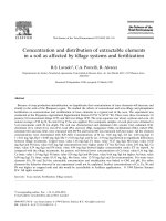
We derive the demographic composition of car use patterns from the Austrian micro-
census of June 1997. First, we categorize households according to five compositional
variables, or combinations of variables: (1) age of household head, (2) age and sex of
household head, (3) size of household, (4) number of adults and children in the
household, and (5) age of household head and size of household. For each of these five
compositions, we next calculate the mean distance driven by households within each

category of the compositional variable. Calculations are based only on those households
that recorded a positive travel distance during the year preceding June 1997. For instance,
in case of composition (1) we calculate the mean distance driven for households whose
head is aged 18-24, 25-29, etc. years old, and who report a non-zero distance traveled in
the past year. Since the number of households that recorded a positive distance is a subset
(of about 90%) of those households that own a car, we calculate car ownership across the
various levels of each composition in a second step. The results of these calculations are
summarized in Figure 1a -1e.
To verify the sensitivity of travel demand patterns to alternative compositions, Table 1
summarizes the results of a simple ANOVA analysis applied to the variable that
measures the distance driven with the first two cars for each compositional variable. The
F-statistics verify that for all compositional variables, the average distances across the
categories differ significantly. A comparison across the proportions of total variance
accounted for by each model shows that age and size considered independently are
almost equally effective in explaining total variance, while age and size together provide
the best combination of variables among the models tested.
[Table 1 about here]
[Figure 1a-1e about here]
Household age
4
Figure 1a shows a distinct age pattern of car ownership and car use. Car ownership
increases with the age of the household head and reaches a peak of almost 90% for the
40-44 year age group. Thereafter, ownership declines and falls below the 50% mark,
beginning with the 70-74 year age group. The pattern of car use is very similar to the car
ownership pattern in that car use first increases up to the late middle ages and declines
thereafter. These age patterns are driven by several factors. Generally, household size
first increases with the age of the household head and starts to decline again at older ages.
One-person households account for more than 50% of households aged <25 and >75, but
for less than 20% of households aged 35-49. Labor-force participation, and consequently
the necessity to commute and means of travel, also vary with the age of the household

head. Labor-force participation increases from about 70% for households aged <25 to

4
Hereafter, we use “household age” to mean the age of the household head. Note that cohorts of
households defined using this definition of age do not necessarily constitute an identical group of
households over time, since reorganizations of membership can add or subtract households from a cohort.
5
93% for households aged 40-44, then declines to <10% for households aged >65. Cohort
effects may also be involved. Today’s middle-and young-aged generation has grown up in
times when car ownership has been the norm rather than the exception. As these cohorts
age, we may expect to see a disproportionate increase in car ownership and car use
patterns among the older generation.
Gender differences in car ownership and car use patterns persist across all ages (Figure
1b). While car ownership is about 20 % lower for female- as compared to male-headed
households up to age 50, this difference increases to 45% for older households (e.g. while
only 15% of female-headed households at age 75-79 own a car, 60% of male-headed
households in the same age group do so ). The divergence in ownership with increasing
age may partly be caused by a cohort effect. However, we also observe a clear difference
in labor-force participation and household size across age between male- and female-
headed households. While among male-headed households aged 55-59 years about 61%
of all household heads are in the labor-force, only 26% of all female household heads in
the same age category are employed. Corresponding figures for households aged 40-44
are 94% and 86%, which is a much smaller gap. Moreover, the percentage of single
person households is higher among female-headed households, particularly for the older
age groups. 82% of female-headed households in the age category 70-74 are single
person households; the corresponding figure for male-headed households is 13%. At age
25-29 this difference is much smaller, with 47% of female and 34% of male households
being single households. Both trends, the lower female labor-force participation rate and
the higher prevalence of single person households, may partly explain the gender gap in
car ownership. Since both differences increase with age, this may also explain the

increasing gender gap across age.
While gender difference in car ownership increases with age, car use patterns of female-
and male-headed households become more similar with the age of the household head.
The gap in car use at younger ages is most likely driven to a large extent by the fact that
female-headed households not only tend to be smaller but are also more likely to be
single adult households. For households aged 25-44 that own a car, 49% of female-
headed households and only 33% of male-headed households have a single adult. In
contrast, for households aged > 65, the corresponding figures for female-and male-
headed households are nearly identical (92% and 95%, respectively). One might suspect
that the fact that the gender gap in car use patterns declines with age is also influenced by
narrowing gender gaps in labor-force participation as well as size and/or number of adults
among households that own a car. However this hypothesis is not supported by the data.
Household size
Household size (Figure 1c) positively affects car ownership and car use. Part of the
household size effect reflects an age effect. Smaller households are more likely to be
headed by younger and older people (rather than the middle-aged) and these are the age
groups for which both car ownership and use are lowest (Figure 1a).Car ownership
increases most between households of size one and two. For car use, the greatest increase
is between households of size two and three. The former result may be explained by an
6
age effect. Among single-person households, 19% are young (25-34 ) and 34% are old
(70-80+) households. The corresponding figures for two-person households are shifted
away from older households - 14% and 22% respectively. Together with Figure 1a, these
compositional changes contribute to the increase in car ownership between one- and two-
person households. The sharp increase in mean distance driven between households of
size two and three may be attributed to a compositional change in age. Three- person
households are more predominantly middle-aged than are one-and two-person
households. For example, 74% of all three-person households that own a car are headed
by persons aged 30-59 (the age category with the highest mean distance driven, Figure
1a), whilst only 58% and 52% of one-and two-person households respectively fall into

this age category. Moreover, the age definition among two-person households that own a
car is generally older .While only 24% and 26% of one and three-person households
respectively that own a car are in the age group 55-74, the corresponding number for
households of size two is 46%.
Household composition
Household size may be too crude a measure since it aggregates households of the same
size, independent of the age of household members. A three-person household may either
consist of three adults, two adults and one child, or one adult and two children; each of
these combinations might be expected to have different transportation demands. (We use
age 18, the age at which a driving license can be obtained in Austria, as the age that
distinguishes between adults and children.) Figure 1d represents a composition of car
ownership and car use that distinguishes between adults and children. From these figures
we may draw the following conclusions. Firstly, adult only households have the highest
rates of car use and ownership across all household sizes. Secondly, within a given
household size, the presence of one or more children reduces car ownership only for
single adult households ( i.e. for households of size two, three and four, we observe a
marked decrease in car ownership pattern only if there are one, two or three children
present, respectively). In short, single parent households have the second lowest car
ownership after single adult households. Since the latter group of households is
composed of old-and young-aged households (compare our discussion to Figure 1a and
1c) it is not surprising that single adult households have the lowest car ownership.
Thirdly, single parent households also have the lowest car use within each household
size. However, while the presence of two or more children does not essentially effect the
car ownership pattern for households of size >4, it markedly reduces car use.
Our results indicate a strong correlation between age of the household head and
household size. Figure 1e therefore presents car use and car ownership patterns across
age and household size. From these results we may conclude that the age pattern of
transportation demand aggregated over all household sizes mainly reflects the age
patterns observed for households of size one and two. Larger sized households generally
show a more stable age pattern. This may be explained by the fact that firstly, larger sized

households are less likely to be headed by persons of very young or alternatively very old
age and secondly, that these households are more likely to be composed of two
generation households. In the case of multi-generation households, the age pattern of car
7
ownership and car use reflects the mix of the life-cycle transportation demand of several
generations. In case of single adult households (more prevalent among smaller household
sizes), the age pattern of car use and car ownership is tied to the life-cycle demand
pattern of only one generation. Seen from an alternative perspective, Figure 1e also
shows that the difference in transportation demand between household sizes varies across
the age of the household head. For middle- and particularly older-age groups, the
difference in transportation demand between household sizes is most pronounced. Given
that we are likely to observe a tendency towards smaller sized households and an ageing
population in the future (see section 4), a composition by age as well as household size
seems to be appropriate for long term projections of transportation demand.
4. Household projections
To understand the influence of key demographic factors on car use in the long term, it is
important to apply population and household projections that can provide detailed
information on changes in demographic determinants in the future. However, conducting
a consistent, simultaneous, dynamic population and household projection has remained
difficult for a long time. As stated by Lutz et al. (1994, p. 225), “…there is no feasible
way to convert information based on individuals … directly into information on
households. Even if these two different aspects could be matched for the starting year
there is no way to guarantee consistent changes in both when patterns are projected into
the future”. Previous studies on population-environment interactions, particularly those
on the development of population and energy use, limit their analysis to separately
treating population at the individual and household level. Those attempting to combine
household and individual level information apply a static approach, mostly utilizing the
well-known “household headship” rate method. However, the link between the headship-
rate and underlying demographic parameters is unclear, given the difficulty in
incorporating assumptions about future changes in demographic events. Moreover, this

approach lumps all other household members into the very heterogeneous category "non-
head". Therefore, it can not provide detailed information on changes in demographic
factors that may be important for future energy use projection. A dynamic population and
household projection is obviously desirable. The advancement in theories and methods of
family demography have improved our capacity to achieve this. Dynamic micro- and
macro- household models (e.g. Hammel et al., 1976; van Imhoff and Keilman, 1991;
Zeng et al., 1997, 1999) have been developed. Benefiting from methodological advances
in multi-state demography, Zeng (1991) constructed a family status life-table by
extending Bongaarts (1987) nuclear status life-table model. Building on this family status
life-table, the dynamic projection model “ProFamy” has been developed to
simultaneously and consistently project future household and population changes which
can match our research purposes.
By applying the ProFamy model, we conducted a dynamic household and population
projection for Austria for the period 1996-2046. From the 1996 micro-census data we
derived the baseline population for running ProFamy. Based on data from the 1995-96
Austrian Fertility and Family Survey (FFS) and the 1996 micro-census, we constructed
standard schedules that determined future transitional patterns by age, sex, and marital
8
status. Standard schedules not derived from the two sources were obtained from
alternative data sources of Statistic Austria. From the 1996 micro-census, FFS and
Statistic Austria, we also derived summary measures of the base year to provide
information on the number of transitions in the starting year. For the summary measures
of future years, we applied the assumptions of the medium variant as suggested in the
latest projections of Statistic Austria (Hanika, 2000) for the total fertility by parity, life
expectancy, mean age at childbearing and external migration (cf. Table 2). Other
parameters, such as marriage, remarriage, cohabiting, divorce, leaving parental home and
sex ratio at birth were maintained over the whole projection period. For a detailed
introduction to the methodological issue of the household projection see Appendix A.
[Table 2 about here]
[Figure 2a-2g about here]

Our projection results indicate a moderate increase in population size and number of
households between 1996 and 2035 (Figure 2a), followed by a decrease in both after
2035. Moreover, changes in the number of households will be more pronounced than
changes in the population size. From Figure 2b, we observe a process of population aging
for Austria over the next five decades. The proportion of children will continuously
decline and the number of adults will grow faster than the total population in 1996-2035
and decrease slower than the total population later on. However, among adults, the
percentage of the elderly will increase. In particular, the elderly aged 75-84 and > 85 are
groups whose population share will increase the most.
Population aging also implies that households will age
5
( i.e. the age of the household
head will increase). Figure 2c clearly shows that the peak of households by age of
household head will move from age 30 in 1996 to age 40 in 2005, age 50 in 2015, age 60
in 2025, age 70 in 2035 and around age 80 in 2046. This is mainly due to the aging of
baby boomers born in the 1960s.
If we look separately at male-and female- headed households by age of the household
head (Figure 2d and Figure 2e), we generally observe the same trend towards higher ages
of the household head. However, we also notice that the peak age of household heads
becomes less visible in future years among male-headed households, due to higher male
mortality. By 2046, the number of male-headed households is almost evenly distributed
among the late 20s to early 80s age groups. Regarding female- headed households, we
observe a fluctuating pattern of the peak age of household heads across time. In general,
there are two peaks across age for all projection periods; one peak around age 20 and the
other around age 70. This pattern reflects the fact that women tend to leave the parental
home and marry earlier than men, which creates the first peak at around age 20. Women

5
In some developing countries, where the extended family is common, population aging does not
necessarily lead to "aging" of household heads. Since most parents transfer household title to their son

when they get old, the age pattern of household headship rates stays unchanged. In Austria, transition of
household heads between generations is not common, therefore, population aging means "aging" of
household heads.
9
also have a longer life expectancy which forms the second peak in the advanced age
group. However, there is a third peak in the middle period and this peak shifts towards
older ages. This is mainly due to the effect of aging baby boomers. Moreover, for female-
headed households the peak in early age is almost constant across the projection period
while the peak in old age shifts towards older ages. Furthermore, except in the very
young age group (15-19 years) and the advanced older age group (70+), the number of
male headed-households is always greater than the corresponding number of female-
headed households.
Given that the number of households is projected to increase faster than the total
population in 1996-2035 and to decrease slower in 2035-2046, the average household
size is expected to decrease (Figure 2f). The latter will decline from 2.4 in 1996 to 1.95 in
2035 and 1.94 in 2046. Numbers of smaller households (one-person and two-person
households) will continuously increase while numbers of larger households (four- and
more person households) will decrease. The number of three-person households will
increase in the early years of 1996-2010 before decreasing subsequently. This change
mainly reflects our assumption that the total fertility rate will increase from 1.42 to 1.5 in
the period of 1996-2020, and stay constant at a level of 1.5 after 2020. Even though the
fertility rate will increase up to 2020, changes in age structure will drive the number of
three-person household down, starting around 2010.
Figure 2g presents a projection of households by household size and distinguishes
between the number of adults and children for each household size category. The
projections show that one- and two-adult households will experience significant and
continuous growth over the next five decades, with all of the growth attributable to
households without children. Three-adult households will increase initially in 1996-2015
but decrease afterwards. Focusing on changes in households by size and by age of
household head, one can see that an increasing number of one and two-adult households

will be mainly elderly. Furthermore, the number of households with children will decline
with the exception of single parents with one or two children for the period 1996-2005.
Household projections under alternative future demographic scenarios
Taking into account the uncertainty of future demographic parameters, we also present
household projections for alternative developments of mortality, fertility and union
dissolution patterns.
In the case of fertility and mortality, we apply the low and high variant as given by
Statistic Austria (see Table 3 and Appendix A, summary measure) in addition to the
medium level of fertility and mortality applied in Figure 2. For the alternative union
dissolution scenarios we cannot refer to any prevailing scenarios. We therefore construct
a low and high union dissolution scenario, assuming that Austria follows the Italian (low
union dissolution scenario) or the Swedish pattern (high union dissolution scenario) of
union dissolution by the year 2046. Between 1996 and 2046 we apply a linear
interpolation. More specifically, we refer to the Family and Fertility Survey conducted in
several European countries in the 1990s and co-ordinated by the Population Activities
10
Unit of the UN Economic Commission for Europe (UN ECE PAU). According to these
data, out of 19 European countries (cf. Prskawetz et al. 2002) Swedish women of birth
cohort 1952-59 have the highest union dissolution rate by age 35 - about 1.5 times that of
their Austrian counterparts. At the other end of the scale, Italian women of the same birth
cohort have the lowest union dissolution rate by age 35 - about 0.26 times of that of their
Austrian counterparts.
[Table 3 about here]
[Figure 3a-3c about here]
In Figure 3 we have assembled selected results of household projections based on
alternative fertility, mortality and dissolution scenarios. A comparison across projections
by population size, number of adults and number of households (Figure 3a) show that
predicted population size will be most sensitive to the assumed fertility development.
This can be explained by the fact that a change in fertility today has a multiplier effect
since children born today will have children themselves in the future. The projected

number of adults will initially be sensitive to changes in mortality patterns and only
around 2025, when the changes in fertility have worked their way through the ages we
can observe the impact of fertility changes on the number of adults as well. Changes in
the rate of union dissolution only have an impact on the projected number of households.
6
In Figure 3b we plot the projected share of households for three age groups of the
household head. The share of household heads in each of three broad age groups is not
overly influenced by alternative demographic scenarios. We observe a pronounced
decrease in the percentage of middle-aged household heads, and an increase in the
percentage of old-aged household heads, for each demographic future scenario (i.e. the
ageing process in households will not be overly affected even under alternative fertility
and mortality assumptions in the future). However, projected changes in household size
are more sensitive to alternative scenarios. Figure 3c illustrates a general increase in one-
and two-person households while households of size three or more are declining over
time. By definition, the share of one- person households is most sensitive to alternative
dissolution scenarios. This result is a combination of higher dissolution rates among
couples without children and the fact that after a dissolution, at least for one partner, the
new household form will be most likely a one-person household. Households of size two
and more are most sensitive to fertility and dissolution scenarios.
From Figure 3 we may conclude that alternative fertility scenarios will primarily effect
total population size and the share of households of size two and more. Alternative
mortality scenarios will have a strong impact on the projected number of adults.
Compared to the fertility scenarios, the impact of mortality changes on the distribution of
households by age of household head and size of household will be less pronounced.
Changes in the dissolution patterns will mainly influence the projected number of

6
This result mainly follows from our assumptions of future levels of TFR and life expectancy at birth
which are the same as for the medium scenarios. We are aware that changes in union dissolution rate may
induce important effects on TFR and life expectancy. However since we lack appropriate data we had to

pose this assumption.
11
households and will have a pronounced impact on the distribution of households by size.
Overall, alternative demographic scenarios will not revert the trends towards older and
smaller sized households. However, a composition of households by size is more
sensitive to demographic scenarios as compared to a composition of households by age of
the household head.
5. Projections of transportation demand
Our cross-sectional analysis shows that household car ownership and use varies
substantially with the age and sex of the householder as well as size (particularly for the
one to three- person households), and with some aspects of household composition. One-
adult households, especially single parent households, differ from households with two or
more adults. Moreover, we found that size- effect is partly caused by changes in age
composition across households of various sizes and vice versa. More specifically, while
the difference in car ownership and car use across age is most pronounced among
households of size one and two, household size is most significant for middle and old
aged households.
The household projections demonstrate that the age distribution of householders will
become significantly older, household size is likely to shift decisively toward one- and
two- person households at the expense of large households. Households without children
will account for essentially all of the growth in total numbers of households.
To arrive at a projection of car use by various demographic decompositions, we combine
the results of the household projections with the corresponding cross sectional
decomposition of car ownership and car use patterns. For each category of a demographic
decomposition, we multiply the projected number of households with the car ownership
rate and the mean distance driven. We neglect any behavioral changes in transportation
demand patterns across various demographic compositions. In other words, this exercise
highlights the role of changing demographic structures
7
but neglects any changes in

transportation demand across various demographic groups.
Change in car use under different demographic compositions; medium variant of the
household projections
[Figure 4 about here]
In our first step, we apply the medium variant of the household projections and plot the
change in car use patterns relative to 1996 for each projection step and each demographic
composition (Figure 4). To interpret these results, it is helpful to begin with the projection
based on constant per capita car use multiplied by projected population size. This
projection ignores any compositional changes in the population and may therefore be
regarded as the benchmark for comparison of alternative projections that take into
account a compositional change of some kind (e.g., household size or age of household

7
Actually in this study we take into account only a few but not all possible changes in behavior of
household formation and dissolution.
12
head). The degree to which these alternative projections differ from the benchmark can
be taken as an indicator of the importance of accounting for the compositional variable
used in the alternative projection. The effect of adding additional compositional variables
(such as adding gender to age) can be measured by examining whether projections
incorporating both variables differ substantially from projections with just the primary
variable.
We examine two general groups of alternative projections: (a) those that take age
composition (and additional variables) into account, and (b) those that take household
size (and additional variables) into account. Accounting for the age structure of
household heads, we obtain a projected car use pattern that is substantially different in
level and pattern than the benchmark projection (Figure 4), namely that car use increases
through 2020 to a level about 12% higher than the benchmark and then decreases to end
up about 4% higher in 2046. This pattern can be explained by the aging of the baby boom
generation (cf. Figure 2c) which implies a movement along the “hump-shaped” car use

pattern by age as depicted in Figure 1a - an effect that is missed by the constant per-
capita benchmark projection. Note that a simpler means of capturing age effects – (a
projection based on number of adults multiplied by per adult car use) is not able to fully
capture this age effect. While it projects greater car use than the benchmark scenario, due
to the faster growth of numbers of adults as compared to total population, it treats all
adults as a homogenous group and misses the fact that most of the growth in adults before
2020 will be in age categories with relatively high car use, while growth thereafter will
increasingly shift to older age categories with relatively low car use.
Considering the gender of the household head in addition to age yields a slightly higher
projected car use compared to the projection based on age alone. This increase is due to
the fact that male-headed households have a higher car use than female-headed
households. However the effect is small: car use is never more than 3% higher when
gender is taken into account in addition to age.
Accounting for household size alone yields a projection that follows the general trend of
the benchmark case but peaks about 4% higher in 2025. This result is driven by the shift
toward smaller household sizes: while smaller households have lower car use than larger
households , the increase in the number of smaller households is greater than the decrease
in the number of larger households, more than compensating for this effect and leading to
a net increase in aggregate car use.
8
A simpler means of accounting for household size
applied in previous studies is to multiply the projected number of households by the
average per household car use. The projected number of households implicitly takes into
account changes in average household size, since it is equal to the population size divided
by average household size. Figure 4 shows that this approach yields the highest of all the
projections, peaking about 20% higher than the benchmark case in 2030. The result is
driven by the fact that this method accounts for shifts in household size in the

8
Alternatively, the effect can be explained by the fact that smaller households have larger per capita car use

and therefore a compositional shift in the population toward smaller households leads to greater aggregate
car use.
13
demographic projection, but does not account for the fact that smaller households have
lower car use; it applies constant car use per household throughout the projection.
When household composition, defined as number of adults versus children, is added to
household size, projected car use increases by just a few percent. This relatively weak
influence may be the result of two offsetting effects: more adult-only households,
exerting upward pressure on car use rates, and an increasing share of single-parent
households, exerting downward pressure on car use (cf. Figure 1d).
We conclude by applying a composition that differentiates between household size and
age of household head combined (cf. Figure 1e). This projection yields results that are
substantially different in both pattern and level from the projections accounting for each
variable alone. Relative to the projection incorporating age alone, car use is lower by up
to 7%. The age-only projection does not account for the fact that the shift toward older
households will also involve a shift toward smaller households with lower car use.
Relative to the projection incorporating size alone, the projection incorporating age + size
is higher through 2026 and lower thereafter. The size-only projection does not account
for the baby boom-driven age effect which drives car use first higher, and then lower,
than it otherwise would be. Adding gender of the household head in addition to the age of
the household head and the size of the household yields slightly higher car use but does
not effect the general shape of the projected car use pattern.
Taken together, these results imply that accounting for both age and size of households is
warranted in projecting future car use. Adding gender of the householder and the
adult/children composition of households has less effect. In addition, simple means of
accounting for age and size such as using number of adults and number of households are
insufficient to capture these demographic effects.
Change in car use under different demographic compositions and alternative future
demographic scenarios
The extent to which a particular compositional variable affects future car use depends on

the household projection employed. Under alternative assumptions about fertility,
mortality, or union dissolution, the projected distribution of households by age, size,
gender, and composition will change. As a result, the conclusions regarding the most
important compositional variables to include in projected car use could also change.
To explore this possibility, we extend our analysis by investigating the sensitivity of
projected car use to the alternative household projections presented in section 4.
9
[Figure 5a-5e about here]

9
Of course, changes in the cross-sectional pattern of car ownership and mean distance driven may have an
equally important influence on projected car use. However since we lack information on changes in car use
patterns across cohorts we restrict our analysis to the sensitivity of car use with respect to alternative
household projection scenarios which can be constructed straightforward by assuming alternative future
time paths of demographic parameters.
14
We present our findings as follows. In the case of only one compositional variable we
plot the change in projected car use relative to a projection based on population size alone
(Figure 5a). If we have two or three compositional variables, we plot the ratio of the
projection including both or all three variables to the projection including just one or two
variables (Figure 5b, 5c, 5d and 5e). This approach controls for the differences in
population size across scenarios with different demographic assumptions. Results can
then be interpreted directly in terms of the importance of the compositional effect being
tested, independently of the effect of differences in population size.
The results of Figure 5a imply that household age and size will be significant in all of the
future demographic scenarios, since in all cases projected car use differs as compared to a
projection based on population size alone. The effect of household size is smaller and not
as sensitive to demographic conditions, leading to a 3-5% increase in projected car use
depending on the household scenario. The effect of household age is more pronounced,
and more sensitive to the household scenario, peaking at 10-15% above the benchmark

projection and ending at -3% to +12% in 2046, depending on the demographic
assumptions.
The results can also be used to examine the main causes of the sensitivity of car use to
alternative assumptions. For example, the differences in car use between the high and low
mortality scenario, after controlling for population size, are not very pronounced over the
time period of the projection. Changes in mortality shift the distribution of households
between middle- and older-aged categories (see Figure 3b). For example, lower mortality
leads to a greater proportion in older households and a smaller proportion in middle-aged
households, reducing overall car use since older households drive less. The differences in
projected car use are small initially, since the increase in older households is concentrated
in those households with driving patterns the most similar to the middle aged (i.e., the
youngest households within the old-age group). Continued low mortality eventually leads
to greater concentrations in the oldest households with the lowest level of driving. As a
result, near the end of the projection period lower mortality is leading to an increasingly
strong effect on total car use.
Differences in car use (controlled for population size) among the high and low fertility
scenario are much more pronounced. Alternative fertility scenarios change the share of
middle-aged households, and total car use is sensitive to this change. Lower fertility, for
example, leads to a smaller share of young households, and a larger share of households
in both the middle- and old-aged groups. The effect of the increase in middle-aged
households (with high car use) dominates, and total car use increases. Projected changes
in car use are even more pronounced if we assume alternative dissolution patterns, since
these alternative scenarios lead to the largest shifts in the distribution of households by
age (Figure 3b). For example, higher dissolution rates shift the distribution of households
toward the middle-aged group, which has relatively high car use, leading to an increase in
overall car use.
15
In Figure 5b and 5c we consider the effect of adding a second compositional variable to
either the age of the household head or the size of the household. We plot projected car
use relative to projections that account for age of household head or household size only.

Results confirm conclusions reached in the previous section regarding the relative
importance of different compositional variables. Adding sex to age (Figure 5b) results in
relatively small changes in car use, although in the low dissolution case the effect is the
largest, reaching 4% by the end of the projection period. Lower dissolution rates lead to a
larger share of male-headed households, which have higher car use than female-headed
households. However, this result does not include the size effects associated with
changing dissolution rates, which would act in the opposite direction. Adding size to age
has a pronounced effect in all scenarios, although it is considerably lessened in the low
dissolution scenario (and considerably increased in the high dissolution scenario).
Adding composition (by adults vs. children) to size (Figure 5c) has a relatively small
effect in all scenarios while adding age to size has a substantial effect in all cases.
We conclude by considering three compositional variables: age and sex of household
head together with household size (Figure 5d and 5e). Adding gender of the household
head (in addition to age and size of the household) does not change the pattern of future
car use and this is independent of the future demographic scenario we assume (Figure
5d). Compared to Figure 5b, part of the gender specific effect has already been taken up
by the compositional variable household size such that by adding gender changes in car
use across alternative future demographic scenarios are very small. The importance to
distinguish by household size (in addition to age and sex) is verified again in Figure 5e.
However, compared to Figure 5b, the effect of adding size across alternative future
demographic scenarios is smaller if gender has already been considered in addition to
age.
Our results confirm the robustness of our initial conclusion that household age and size
are important compositional variables to include in projections of future car use. By
adding gender to a composition by age and size (Figure 5d), not much additional change
in car use can be observed. We may therefore conclude that age and size are indeed the
most appropriate compositional variables within our set of household characteristics that
we consider. With respect to the alternative future demographic scenarios our results
indicate that the quantitative relevance to a specific demographic composition may
change under alternative demographic future scenarios while the qualitative shape

persists.
6. Conclusions
Demand patterns for transportation with private vehicles are closely connected to
demographic variables, including those reflective of life-cycle stages. We find, as have
previous studies, that demand for household transportation varies significantly by
different subgroups of the population defined by household characteristics such as age
and gender of the householder, size, and age composition. By combining cross-sectional
variations in travel behavior by demographic characteristics with a new projection of
16
households in Austria, we illustrate that future compositional changes in the population
by living arrangements could substantially influence demand for transportation.
Furthermore, we show that projections are sensitive to the particular type of demographic
disaggregation employed. These results suggest that demographic disaggregation not only
has the potential to improve forecasts of future travel demand, but also to emphasize the
importance of careful choice of variables by which to disaggregate the population.
Demographic changes could be important for at least two reasons in addition to those
analyzed here. First, we assume that category-specific car ownership and use rates remain
constant. If, however, these rates changed differentially across categories, the effect of
compositional changes on aggregate demand could be either exacerbated or dampened.
Second, one of the reasons why category-specific rates might be expected to change is
the likely existence of cohort effects (a demographic variable). For example, as baby
boom women age, they are likely to increase the rate of car ownership in elderly age
groups.
[Figure 6 about here]
Whether our results indicate that compositional changes could have a substantial
influence on future travel behavior needs to be judged relative to the influence of other
factors, including behavioral and technological changes. Referring to data provided by
the Austrian environmental ministry (Figure 6), vehicle kilometers traveled (VKT) per
adult is forecasted to increase by about 62% during the period 1996 to 2030 compared to
an increase of 155% over a historical period of similar length from 1967 to 1996.

10
At the
same time, changes in energy efficiency and transportation fuels could lead to an
improvement in CO2 emissions per vehicle kilometer of 40% over the period 1996 to
2030 compared to an improvement of only 15% for the historical period 1967 to 1996.
Compared to these projected changes in VKT and technological factors, our predicted
changes in car use resulting from compositional changes are modest. Taking the
projection by household age, sex and size as an example and considering the medium
variant of the household projections, differences from the projection which ignore
composition (the constant per capita projection) do not exceed 8%. For an application
forecasting aggregate transportation energy use 50 years into the future, an 8%
adjustment is relatively small given the scope for changes driven by behavioral or
technological change. On the other hand, the projection with composition shows a
different dynamic which may be important, with demand peaking earlier and then
declining, in sharp contrast to the constant per capita projection and the projections
presented in Figure 6. In addition, the difference between the two projections is nearly
8% in the short term (2010-2015). Over this shorter time horizon, an 8% absolute
difference in projected demand is likely to be much more important in judging the
difficulty of meeting greenhouse gas emission reduction targets, or for planning for
changes in demand for road capacity, for example.

10
We would like to thank Günther Lichtblau (Austrian environmental ministry) and Alexander Hanika
(Statistic Austria) who provided the data on VKT, energy efficiency and the Austrian adult population.
17
References
Bongaarts, J. (1987) The projection of family composition over the life course with family
status life- tables. In John Bongaarts, Thomas K. Burch, and Kenneth W. Wachter (eds.)
Family demography: Methods and their application, edited by International Studies in
Demography, 189-212, New York: Oxford University Press.

Buettner, T. and Grubler, A. (1995) The birth of a "green" generation?:Generational
dynamics of consumption patterns. Technological Forecasting and Social Change 50,
113-134.
Carlsson-Kanyama, A. and Linden, A L. (1999) Travel patterns and environmental
effects now and in the future: Implications of differences in energy consumption among
socio-economic groups. Ecologcial Economics 30, 405-417.
Dahl, C.A. and Sterner, T. (1991) Analysing gasoline demand elasticities: A survey.
Energy Economics 13(3), 203-210.
Doblhammer, G., Lutz, W. and Pfeiffer, C. (1997) Tabellenband und Zusammenfassung
erster Ergebnisse: Familien- und Fertilitätssurvey (FFS) 1996. Österreichisches Institut
für Familienforschung, Vienna, Austria.
Grenning, L.A. and Jeng, T.H. (1994) Lifecycle analysis of gasoline expenditure patterns.
Energy Economics 16(3), 217-228.
Greening, L.A. et al. (1997) Prediction of household levels of greenhouse gas emissions
from personal automobile transportation. Energy 22 (5), 449-460.
Hammel, E.A., Hutchinson, D. W., Wachter, K.W., Lundy, R.T. and Deuel, R.Z. (1976)
The SOCSIM Demographic-Sociological Microsimulation Program, Berkeley, Institute
of International Studies, University of California (Research Series No. 27).
Hanika, A. (1996) Volkszählung 1991: Paritäts-Fruchtbarkeitstafeln, Statistische
Nachrichten 6/1996, 426-431.
Hanika, A. (1999) Realisierte Kinderzahl und zusätzlicher Kinderwunsch: Ergebnisse des
Mikrozensus 1996, Statistische Nachrichten 5/1999, 311-318.
Hanika, A. (2000) Bevölkerungsvorausschätzung 2000-2050 für Österreich und die
Bundesländer, Statistische Nachrichten 12/2000, Statistik Austria, 977ff.
Kayser, H.A. (2000). Gasoline demand and car choice: Estimating gasoline demand
using household information. Energy Economics. 22(3), 331-348.
18
Lutz, W. (ed., with ass. eds.: Baguant, J., Prinz, C., Toth, F.L. and Wils, A.B.) (1994),
Population - Development - Environment: Understanding their Interactions in Mauritius,
Berlin, Springer-Verlag.

U.S. National Research Council (NRC) (1997) Toward a Sustainable Future: Addressing
the long-term effects of motor vehicle transportation on climate and ecology. Special
Report 251. National Academy Press, Washington, DC, USA.
O’Neill, B.C. and Chen, B. S. (2002) Demographic determinants of household energy use
in the United States, in W. Lutz, A. Prskawetz and W.C. Sanderson (eds.) Population and
Environment: Methods of Analysis, A Supplement to Vol. 28 of Population and
Development Review, New York, Population Council, 53-88.
Prskawetz, A., Vikat, A., Philipov, D. and Engelhardt, H. (2002) Pathways to Stepfamily
Formation in Europe: Results from the FFS. Mimeo, Max Planck Institute for
Demographic Research.
Pucher, J., Evans, T. and Wenger, J. (1998) Socioeconomics of urban travel: Evidence
from the 1995 NPTS. Transportation Quarterly 52(3), 15-33.
Schipper, L., Bartlett, S., Hawk, D. and Vine, E. (1989) Linking lifestyles and energy use:
A matter of time? Annual Review of Energy and the Environment 14, p. 273.
Spain, D. (1997) Societal trends: The aging baby boom and women’s increased
independence. Report prepared for the U.S. Dept. of Transporation, Order no. DTFH61-
97-P-00314.
Statistic Austria (1998) Energieverbrauch der Haushalte 1996/97: Ergebnisse des
Mikrozensus Juni 1997, Vienna, Austria.
UN ECE PAU. FFS model questionnaire for women. Available at
/>van Imhoff, E. and Keilman, N. (1991), Lipro 2.0: An Application of a Dynamic
Demographic Projection Model to Household Structure in The Netherlands,
Amsterdam/Lisse and Berwyn PA, Swets & Zeitlinger Inc.
Zeng Yi (1991), Family Dynamics in China: A Life Table Analysis, Wisconsin, The
University of Wisconsin Press.
Zeng, Yi, Vaupel, J. and Wang, Z. (1997) A Multidimensional model for projecting
family households with an illustrative numerical application. Mathematical Population
Studies, Vol. 6, No. 3, 187-216.
19
Zeng Yi, Vaupel, J. and Wang, Z. (1999), Household projection using conventional

demographic data, in W. Lutz, J.W. Vaupel and D.A. Ahlburg (eds.), Frontiers of
Population Forecasting, A Supplement to Volume 24 of Population and Development
Review, New York, Population Council, 59–87.
20
Appendix A: Methodology of household projection
ProFamy is a software package for a multi-dimensional, macro-dynamic model for
projecting households and population. In the ProFamy model, the individual is chosen as
the basic unit of the projection. The individuals in the starting population are derived
from a census or survey. Individuals in the projected population are classified according
to 8 dimensions of demographic status: age, sex, marital status, parity, number of
children living at home, co-residence with parents, household type (private or collective),
and area of residence (rural or urban). Characteristics of the reference person (or
household “markers”) are applied to derive the distributions by household type and size.
Because the model deals with two sexes, children and parents, a harmonic-mean
procedure is used to ensure consistency between females and males, and children and
parents. At the end of the projection, the numbers of non-familial members who co-reside
with the reference persons is estimated indirectly (Zeng et al., 1997).
Baseline population and status identification
The 1996 Austrian micro-census, which includes a sample of the Austrian population of
the order of 64,183 individuals
11
, provides the baseline population for our household and
population projection. In order to adjust this sample to get the correct total population
size by age, sex, and marital status, we need to provide ProFamy with information on the
total population in the starting year. The 100% tabulation of the total population
(8,054,423) classified by single year of age, sex and marital status is derived by applying
the population weights provided in the 1996 micro-census. Table A.1 summarizes the
status of individuals as used in our projections.
[Table A.1 about here]
This information, as derived from the 1996 micro-census, serves as the input for

BasePop, the sub-program of ProFamy, in order to produce the base population for
projections in ProFamy.
Standard schedules
The basic structure of the demographic accounting equation in ProFamy is as follows:
number of persons of age x+1 with status i at time t+1 =
(number of persons of age x with status i at time t) +
(number of entries into status i which occur in the year (t, t+1) among persons of age
x+1 at time t+1) –
(number of exits out of status i which occur in the year (t, t+1) among persons of age x
at time t).

11
It should be noted that, there are some individual cases in the micro-census data set containing no
information required. Those cases with missing value are excluded from the baseline population.
Consequently, 57,030 out of 64,183 are used in the final sample for ProFamy.
21
The number of demographic events in year (t, t+1) and at ages x or x+1 is calculated as
the number of persons aged x and at risk of occurrence of the event in the year, multiplied
by the projective probability of occurrence of an event that leads to a status transition in
the year (t, t+1) and at age x or x+1 in completed years, fitting in a period-cohort
observational plan for analysis and projection.
12
It is obvious that the standard schedules
defined by age-, sex-, (sometimes parity-, and marital-status-) specific probabilities (or
rates)
13
are extremely important for the projection results.
To derive the standard schedules for the various events we use three sources:
The 1996-1997 Austrian Fertility and Family Survey (FFS) contains detailed information
on partnership formation and dissolution, childbearing, leaving parental home, migration,

and other events, based on a retrospective investigation of 6120 individuals aged 20-54
during the period December 1995 up to May 1996. Applying the method of survival
analysis, we derive the following standard schedules from the FFS data:
(1) Probability of leaving parental home
(2) Transition probability from single to married
(3) Transition probability from single to cohabiting
(4) Transition probability from cohabiting to married
(5) Transition probability from cohabiting to single
(6) Transition probability from married to divorced
(7) Transition probability from divorced to cohabiting
Given the small sample size, the FFS data did not allow for the construction of standard
schedules for the transition probability from widowed to cohabiting. For the latter
transition probability, we therefore assume that it is equal to the transition probability
from divorced to cohabiting. A further shortcoming of the FFS data set is the fact that it
only includes individuals up to age 54. It is un-reasonable to assume that those aged
above 54 do not get divorced. To solve this problem we used 1996 age- and sex-specific
numbers of divorces from Statistic Austria. Combining these numbers with the number of
married couples derived from the 1996 micro-census data set, we calculated the age- and
sex-specific divorce rate, and used it in constructing the standard schedule of divorce
rates. ProFamy software will automatically calculate the standard schedule for the
transition from married to widowed based on the sex-specific mortality schedules and
differences in age at marriage between men and women.

12
Below, when we use the term probability, we always mean probability according to this definition. In this
approach, the demographic transitions under study are assumed to depend on some (but not all) of the other
statuses at the beginning or the middle of a one-year interval (e.g., giving birth depends on age, parity and
marital status of the mother, but does not depend on co-residence with parents). The adoption of the
computational strategy in the model, which assumes that births occur throughout the first half and the
second half of a year, but other events occur in the middle of the year, will significantly decrease the biases

caused by not considering the interfering events while projecting the occurrences of an event.
13
With regard to the input data, the ProFamy software package allows the standard schedules to be either
occurrence/exposure rates or probabilities. If one chooses to use occurrence/exposure rates, the ProFamy
model will automatically transform all rates into probabilities. In our case, we transformed all standard
schedules, except those for the frequencies of migration, from occurrence/exposure rates into probabilities,
before we used them as input into the model.
22
Although the FFS data set contains information on fertility, the small sample size again
did not permit use of these data to derive standard schedules for fertility. We use the 1996
micro-census data set, which provides detailed information on birth biographies, to
construct standard schedules for parity- and age- specific fertility schedules.
(1) Single women fertility
(2) Cohabiting women fertility
(3) Divorced women fertility
(4) Married women fertility
It is noteworthy that we set 15 as the starting age of giving birth, and parity 5 as the
highest parity. Since the number of births by widowed women is too small in the micro-
census we assumed widowed women will not give any birth in our projection. Similarly,
the number of births of parity 4 and 5 by single and cohabiting women, and of parity 5 by
divorced women are very small and we neglect these births for our projections.
The following standard schedules are provided by Statistic Austria:
(1) Probability of survival
(2) Transition probability from divorced to married
(3) Transition probability from widowed to married
(4) Frequency distribution of immigration by age and sex
(5) Frequency distribution of emigration by age and sex
Summary measure
Base year
While standard schedules offer information on the status transition of the future

population characterized by age, sex, and marital status; summary measures provide the
assumption of the total amount of all transitions in the future years. All these assumptions
should be based on the information from the base year and also start from the base year.
Basically, we obtained information for the summary measures of the base year from the
three sources of deriving standard schedules mentioned above.
(1) From the FFS we calculated the proportion of those who eventually leave the parental
home, the propensity of first marriages, the mean age at 1
st
marriage, the propensity from
married to divorced, the propensity from single to cohabiting, the propensity from
cohabiting to married, the propensity from cohabiting to single, and the propensity from
divorced to cohabiting.
(2) From the 1996 micro-census data we derived the ratio of the non-married women
fertility to the married women fertility.
(3) From Statistic Austria we obtained figures relating to life expectancy at birth, total
fertility rate, number of emigrants and immigrants, sex ratio at birth, and propensity for
the widowed and divorced to remarry. Since we lack proper data to estimate the
propensity of widowed to cohabiting, we assume that it is the same as the propensity for
the widowed to remarry.
23
The total fertility rate by parity derived from the micro-census data is the result of the
combination of different cohorts. It is not adequate to use it to represent the distribution
of total fertility rate by parities. Therefore, we obtained data on total fertility by parities
of the latest cohorts of Austrian women born in 1946-1950 who have experienced
childbearing (Hanika, 1996), and use it to represent the distribution of the total fertility
rate by parities. Moreover, we assume no births given by widowed women.
Numbers for external migrants are obtained from Statistic Austria for the year 1998. We
assume that there is no significant change in terms of external migrants between 1996 and
1998 and apply these numbers to our base population of 1996.
From the base population, ProFamy automatically calculates the proportion of persons

living in collective household by age and sex among those who are not living with
children or parents plus the average number of other relatives and non-relatives of
different households by size.
Future changes
For women's’ mean age at giving birth, the number of external migration, the total
fertility rate and the life expectancy at birth we apply the assumptions as suggested in the
latest projections of Statistic Austria (Hanika, 2000).
The mean age at giving birth is assumed to increase ( following a logistic curve) from
28.14 years in 1996 to 30 years in 2030 and it is kept constant at 30 years from 2030
onwards till 2046.
The external migration (Table A.2) is derived from the population projections by Statistic
Austria.
[Table A.2 about here]
For total fertility rate three assumptions are stated:
(1) The medium variant assumption assumes total fertility rate will increase ( following a
logistic curve) from 1.42 in 1996 to 1.5 by the year 2020, and will maintain at a level of
1.5 till the year 2046.
(2) The low variant assumption assumes total fertility rate will linearly decrease to 1.2 by
the year 2020 and remain constant thereafter.
(3) The high variant assumption assumes total fertility rate will linearly increase to 1.8 by
the year 2020, and remain constant thereafter.
For life expectancy at birth, three further assumptions are stated:
(1) The medium variant assumes an increase that follows a logistic curve: from 74.7 to 80
years for males and from 80.9 to 85.5 years for females in the period between 1996 and
24
2030. For the period between 2030 and 2050, life expectancy is assumed to increase from
80 to 82.5 years for males and from 85.5 to 87 years for females.
(2) The low variant assumes a linear increase from 74.7 to 78.0 years for males and 80.9
to 84 years for females in the period between 1996 to 2030. From 2030 onwards, life
expectancy is assumed to stay constant for both sexes.

(3) The high variant assumes that life expectancy at birth between 1996 and 2030 will
increase linearly to 82 years for males and 87 years for females and increase linearly up
to 86 years for males and 90 years for females until 2050.
For the union dissolution rate, we construct a low and high union dissolution scenario
assuming that Austria follows the Italian (low union dissolution scenario) or alternatively
the Swedish pattern (high union dissolution scenario) of union dissolution by the year
2046 (between 1996 and 2046 we apply a linear interpolation).
According to the 1990 round of the FFS Survey, out of 19 European countries, Swedish
women of birth cohort 1952-59 had the highest proportion of union dissolution by age 35
(0.35); about 1.5 times that of their Austrian counterparts (0.23). Conversely, Italian
women of the same birth cohort had the lowest proportion of union dissolution by age 35
(0.05); about 0.26 times of that of their Austrian counterparts. Thus we form three
scenarios for the whole life proportion of union dissolution by married or cohabiting men
and women, by assuming proportionate changes to the base year of whole life proportions
of union dissolution by married and cohabiting men and women derived from the
1995/1996 FFS data. These are: 0.37 for married women, 0.38 for married men, 0.20 for
cohabiting women and 0.29 for the cohabiting men.
(1) The medium scenario assumes the whole life proportion of union dissolution by
married and cohabited women and men will remain constant at the 1996 level till the end
of the year 2046 of the projection.
(2) The high scenario of union dissolution assumes the proportion of union dissolution
between the year 1996 and 2046 will linearly increase from 0.37 to 0.56 for married
women and from 0.38 to 0.58 for married men, while the proportion will linearly increase
from 0.20 to 0.31 for cohabiting women and from 0.29 to 0.45 for cohabiting men in the
same period.
(3) The low scenario of union dissolution assumes the proportion of union dissolution
will linearly decrease to 0.09 for both the married men and women by year 2046. It
further assumes a decrease to 0.05 for the cohabiting women and 0.07 for the cohabiting
men by year 2046.
All other summary measures are assumed to be constant in the future. By applying this

set of assumptions, we actually assume little changes in the behavior of household
formation and dissolution except that changes in women’s mean age at giving birth and
total fertility rate will to a certain degree affect the timing and volume of household
expansion by childbearing.