Agent-based and analytical modeling to evaluate the effectiveness of greenbelts potx
Bạn đang xem bản rút gọn của tài liệu. Xem và tải ngay bản đầy đủ của tài liệu tại đây (239.2 KB, 13 trang )
Environmental Modelling & Software 19 (2004) 1097–1109
www.elsevier.com/locate/envsoft
Agent-based and analytical modeling to evaluate the effectiveness
of greenbelts
Daniel G. Brown
a,b,
, Scott E. Page
b
, Rick Riolo
b
, William Rand
b
a
School of Natural Resources and Environment, University of Michigan, 430 E. University, Ann Arbor, MI, 48109-1115, USA
b
Center for the Study of Complex Systems, University of Michigan, Ann Arbor, MI, 48109-1120, USA
Received 6 February 2003; received in revised form 8 July 2003; accepted 11 November 2003
Abstract
We present several models of residential development at the rural–urban fringe to evaluate the effectiveness of a greenbelt loca-
ted beside a developed area, for delaying development outside the greenbelt. First, we develop a mathematical model, under two
assumptions about the distributions of service centers, that represents the trade-off between greenbelt placement and width, their
effects on the rate of development beyond the greenbelt, and how these interact with spatial patterns of aesthetic quality and the
locations of services. Next, we present three agent-based models (ABMs) that include agents with the potential for heterogeneous
preferences and a landscape with the potential for heterogeneous attributes. Results from experiments run with a one-dimensional
ABM agree with the starkest of the results from the mathematical model, strengthening the support for both models. Further, we
present two different two-dimensional ABMs and conduct a series of experiments to supplement our mathematical analysis. These
include examining the effects of heterogeneous agent preferences, multiple landscape patterns, incomplete or imperfect infor-
mation available to agents, and a positive aesthetic quality impact of the greenbelt on neighboring locations. These results suggest
how width and location of the greenbelt could help determine the effectiveness of greenbelts for slowing sprawl, but that these
relationships are sensitive to the patterns of landscape aesthetic quality and assumptions about service center locations.
# 2004 Elsevier Ltd. All rights reserved.
Keywords: Land-use change; Urban sprawl; Agent-based modeling; Landscape ecology
1. Introduction
Population increase, decreasing household sizes (Liu
et al., 2003), and increases in area developed per house-
hold (Vesterby and Heimlich, 1991) all contribute to
increase in the amount of land converted for develop-
ment in metropolitan areas throughout the world.
Land development for residential, commercial and
industrial uses at the urban–rural fringe can have a
variety of negative ecosystem impacts, including habi-
tat destruction and fragmentation, loss of biodiversity,
and watershed degradation (Alberti, 2000). Landscape
ecological theory (Turner et al., 2001) suggests that, in
addition to how much development occurs, the extent
of these impacts is determined by where the develop-
ment occurs relative to ecological features and its over-
all spatial pattern.
A number of approaches have been proposed to
minimize the ecological impacts of development, by
manipulating the spatial patterns of development to
minimize sprawl and excess land usage. These approa-
ches include establishment of greenbelts of preserved
lands around cities (Mortberg and Wallentinus, 2000),
clustered or ‘‘new urbanism’’ designs (Arendt, 1991),
which involve increased use of higher density develop-
ment and mixtures of land uses within developments,
purchase or transfer of development rights (Daniels,
1991), and alteration of tax or investment policies
(Boyd and Simpson, 1999), among others. For each of
these alternative strategies, the costs of implementation
need to be considered (Boyd and Simpson, 1999) along
with the long term conservation benefits obtained.
To evaluate the benefits of any given option, the
dynamics of development at the urban–rural fringe and
Corresponding author. Tel.: +1-734-763-5803; fax: +1-734-936-
2195.
E-mail address: (D.G. Brown).
1364-8152/$ - see front matter # 2004 Elsevier Ltd. All rights reserved.
doi:10.1016/j.envsoft.2003.11.012
their linkages to ecological impacts need to be under-
stood. Because the impacts are driven to a large extent by
the location and spatial patterning of the development,
this understanding needs to be spatially explicit. In order
to understand the drivers of urban development and their
possible future impacts on land development, and to
develop scenarios that can be used to test alternative
approaches to minimizing these impacts, a variety of spa-
tial modeling approaches have been employed. The work
of Landis and colleagues (Landis, 1994; Landis and
Zhang, 1998a, b) illustrates a simulation approach based
on discrete choice statistics that focuses on estimating the
likely locations of development. Similarly, Pijanowski
et al. (2002) used artificial neural networks to identify
non-linear interactions between predictor variables and
likely locations of development. Alternative modeling
approaches have focused on how the patterns of develop-
ment evolve through spatial interactions and, in many
cases, have used analogies with physical systems (e.g. dif-
fusion limited aggregation and correlated percolation) to
represent processes of urban growth (Makse et al., 1998;
Zanette and Manrubia, 1997). Cellular models (Clarke
et al., 1997) represent an approach that is intermediate in
realism between statistical location models and physical
analog interaction models, combining some of the
strengths of both.
These powerful simulation models have been used to
evaluate the impacts of a variety of land-use policy
instruments. Each of them represents the land-use state
at each location and the variables and processes that
determine that state. An important next step in the
evolution of land-use models, and improving their util-
ity for policy scenarios, is directly representing the het-
erogeneous set of actors in the land-use change process
(Page, 1999), their decision making processes, and the
physical manifestation of those changes on the land-
scape. Agent-based models (ABMs) serve as tools for
this purpose. Otter et al. (2001) presented an ABM of
land development that includes a reasonable represen-
tation of the different types of agents and that makes
an initial contribution on which further developments
in this area might build. Further, experimentation with
this kind of model can improve our understanding of
how the interaction between landscape characteristics
and the preferences and behaviors of agents might
influence ecological diversity and function.
A key challenge in modeling such multi-agent systems
with agent-based models is providing confidence in the
models’ results (Parker et al., 2003). Often establishing
confidence in a computer model is divided into two steps:
(1) verifying that the computer program is free of ‘‘bugs’’
and correctly implements the conceptual model and (2)
validating the model by showing it generates output that
matches the relevant aspects of the system being modeled
(Kelton and Law, 1991). In practice, carrying out those
procedures is not so straightforward. First, verification of
program correctness cannot be guaranteed for any but
the simplest of programs; thus in practice we can only
increase confidence that a program is correct by a combi-
nation of software engineering and testing techniques
(McConnell, 1993). Second, validation also is a non-triv-
ial exercise, since it involves judgements about how well a
particular model meets the modeller’s goals, which in turn
depends on choices about what aspects of the real system
to model and what aspects to ignore. Critical issues that
must be considered include what level of detail to try to
match (data resolution) and how to handle issues of
‘‘deep uncertainty’’ found in complex adapative systems
(Bankes, 2002).
Because of these difficulties, typical practice is to estab-
lish confidence in the results of a model through a mix of
techniques, most of which contribute to both verifying
and validating the model. Sensitivity analysis and other
‘‘parameter sweeping’’ technique can provide support for
computer program correctness and model plausibility, by
improving understanding of the behavior of a model
under a range of plausible conditions (Kelton and Law,
1991; Miller, 1998). In some cases model calibration is
carried out, i.e. model parameters are adjusted (‘‘tuned’’)
until the model output matches the real world data of
interest. For the calibration to be convincing, we also
must show those parameter values are ‘‘plausible,’’ e.g. by
basing them on empirical data or by arguing that experts
support the ‘‘face validity’’ of the parameters chosen. We
also can ‘‘dock’’ models to other related models (Axtell
et al., 1996), to show the results are common to more
than just one model or implementation.
Beyond simple verification and validation of an ABM,
we also want to be confident that we have a clear under-
standing of the agent-based model’s processes and of the
behavior and results those processes produce. Because
agent-based modeling is a new, potentially valuable
approach to understanding complex phenomena like
settlement patterns, much can be gained from under-
standing the models themselves. Further, such an under-
standing of an ABM is a necessary step in using the
model to understand the fundamental processes in the
(more complex) real world system that the model is meant
to represent.
Because an ABM usually is itself a complex system,
it can take considerable effort to understand even the
simplest of models (Casti, 1997; Axelrod, 1997; Bankes,
2002). Axelrod (1997) argues that simulation is a third
way of doing science, combining aspects of deduction
(knowledge based on proofs from axioms) and induc-
tion (knowledge from observed regularities in empirical
data). That is, the ABM can be viewed as a fully speci-
fied formal system (like the axiomatic basis for deduc-
ing theorem proofs) which, when run, generates
data that requires careful analysis (induction) to under-
stand and summarize. For instance, we can induce
regularities by analyzing the model output in ways
1098 D.G. Brown et al. / Environmental Modelling & Software 19 (2004) 1097–1109
similar to those used on data from a real-world sys-
tem
1
.
In this paper we demonstrate another way to under-
stand the basic processes in an agent-based model and,
by extension, to help us understand processes that may
be at play in the system being modeled. The approach
we use in this paper involves comparing the behavior
of an agent-based model to the behavior of a simpler
mathematical model of land development. This com-
parison has a number of benefits, including:
. By having two separate ‘‘implementations’’ which
both generate the same fundamental results, we
increase our confidence in the veracity of both models;
. The results from the stark mathematical model can
be shown to hold in more general contexts which an
ABM can represent, e.g. spatial heterogeneity, dis-
crete service center distributions and other exten-
sions not amenable to mathematical analysis; and
. The theorems we are able to prove for the math-
ematical model give us deeper insights into the pro-
cesses that generate the fundamental dynamics of
the ABM.
In general, agent-based models may be constructed to
serve as minimal realistic models of real-world complex
adaptive systems. However, the fact that we often cannot
prove theorems about the agent-based models makes for
a shaky foundation. But, if we can both prove theorems
about simplifications of the ABMs and show that the con-
clusions of those theorems hold in more general agent-
based models, we enrich the scientific enterprise.
The comparison of an ABM to a simpler mathemat-
ical model can also be viewed as a kind of ‘‘docking’’
exercise (Axtell et al., 1996). In this case one model is
computational and the other is mathematical (instead
of comparing two computational models), but the basic
goal is the same, i.e. to study the ‘‘ troublesome case
in which two models incorporating distinctive mechan-
isms bear on the same class of social phenomena, ’’
(Axtell et al., 1996, Section 1.1), in part to carry out
‘‘ tests of whether one model can subsume another’’
(Axtell et al., 1996, abstract). As emphasized in Axtell
et al. (1996), a key issue is how to assess the ‘‘equival-
ence’’ of two models. For this paper, we focus on
‘‘relational equivalence’’ between the models, showing
that they both generate the same relationships between
results, e.g. as analogous parameters are varied. If the
models are relationally equivalent, we can be more
confident that (1) the mathematical model helps us
understand the key processes in the ABM, and (2) the
ABM can be viewed as subsuming the mathematical
model, allowing us to study a wide variety of cases that
are mot mathematically tractable.
In summary, in this paper we present several models
of residential development at the rural–urban fringe. In
all models, the common conceptual model consists of
agents choosing where to locate based on preferences
for minimizing distance to services and maximizing aes-
thetic quality of the chosen location. We use the mod-
els to evaluate the effectiveness of a greenbelt, which is
adjacent to a developing area, for delaying develop-
ment outside of the greenbelt. Our one-dimensional
mathematical model focuses on the interactions
between greenbelt location and width, the spatial distri-
bution of aesthetic quality, and the resultant amount
and timing of development beyond the greenbelt. We
explore the model under two different assumptions
about the spatial pattern of service centers. Next, we
implement the same basic mechanisms of the math-
ematical model in a one-dimensional discrete ABM set-
ting. We then demonstrate the flexibility of the ABM
framework by relaxing assumptions and extending the
representation of the system to include (1) a two-
dimensional landscape and (2) an effect of the greenbelt
on the aesthetic quality of the nearby environment.
2. Methods
2.1. Mathematical model
We first construct a one-dimensional mathematical
model of resident settlement choices in the presence of a
greenbelt. We use this model to derive some basic
properties about greenbelts, such as a tradeoff between
the width of a greenbelt, its location and the rate of
development to its right. These basic principles, then, set
the stage for evaluation of dynamics within the agent-
based modeling framework, described in Section 2.2
In the basic model, agents care about two features of
a location x: its distance to services, and its aesthetic
quality, which we denote by q
x
. Aesthetic quality is
defined as the value that residential agents derive from
locations because of their scenic and other natural
amenities. We assume that an agent’s utility from a
location increases in proportion to the location’s
aesthetic quality and decreases in proportion to its
distance to services, and that agents choose to occupy
the location that maximizes utility. In this model, we
assume that there is a finite number of agents.
Each of M agents chooses a location from the set {0,
1, N} at which to live. At most, one agent can live at
each location. Therefore, MNþ1.
F: f0; 1; ; Ng!f0; 1g denotes the locations of
the agents. FðxÞ¼1 if an agent resides at location x and
0 otherwise.
1
The key methodological difference between how we analyze out-
put of agent-based models versus real-world data is that for ABMs
we have less use for formal statistical measures like t statistics,
because we can achieve a trivial kind of statistical significance by run-
ning the model an arbitrary number of times.
D.G. Brown et al. / Environmental Modelling & Software 19 (2004) 1097–1109 1099
A greenbelt (g, w) begins at the location g 2f0;
1; ; N w þ 1g of width w with gM. No agents
may live in the locations fg; ðgþ1Þ; ; ðgþw1Þg.
The purpose of the greenbelt is to keep all of the
agents on one side, in this case to the left. For con-
venience, we will say that an agent at location x resides
left of the greenbelt if x<g and to the right of the
greenbelt if x> ðgþw1Þ. Notice that in our definition
of a greenbelt, we required that gM. Without this
constraint, the greenbelt cannot prevent sprawl.
Given a distribution F, the utility to an agent living at
location x is given by:
Uðx;FÞ¼q
x
sðx;FÞð1Þ
where s(x, F) is the distance from x to services, which
can be a function both of the location of the agent and of
the distribution of all agents.
In our two-dimensional (2D) ABMs, we begin with a
service center on the left most edge of the grid
2
. Sub-
sequent service centers gradually locate rightward as
the population grows (see process description below).
To capture these two characteristics of the service cen-
ters, their bias to the left and their spread with the
population, we consider two distinct cases for the
mathematical model. In the first, we assume that there
is a single service center at the leftmost edge of the
space. This assumption corresponds with the mech-
anism used in the one-dimensional (1D) ABM. In the
second, we assume that the distance to services left of
the greenbelt depends only upon the number of agents
located there. This second case contains two implicit
assumptions. First, the services are evenly distributed
relative to agents left of the greenbelt, and second no
one left of the greenbelt jumps the greenbelt to obtain
services. The first of these implicit assumptions makes
sense provided that services are fairly divisible or travel
costs left of the greenbelt relatively low or equal
3
.We
formalize these assumptions as follows:
Case 1. Left Edge Service Centers (LESC): sðx; FÞ¼x
Case 2. Evenly Spaced Service Centers (ESSC): IfK
agents live to the left of the greenbelt ð
P
g1
y¼0
FðyÞ¼KÞ
then sðx;FÞ¼
nq
K
for x<g, where g is a parameter repre-
senting the density of services.
Under LESC, the utility to an agent at location x<g,
U(x, F) equals q
x
x, under ESSC it equals q
x
nq
K
.
Notice that neither of these assumptions depends much
on the particulars of F. Under LESC, distance is inde-
pendent of F and under ESSC, all that matters is the
number of agents to the left of the greenbelt. Neverthe-
less, we keep the s(x, F) notation because, in our 2D
ABMs, the distribution of services and hence the distance
to them depends explicitly on where agents locate.
To analyze whether a greenbelt prevents sprawl, we
need to compare the utility to the Mth agent living left
of the greenbelt with the utility that the agent could
obtain if it jumped the greenbelt. We assume that if a
single agent lives right of the greenbelt it must cross the
greenbelt to get services. Once the agent crosses the
greenbelt, which is width w, the agent has the same dis-
tance to services as someone living on the left edge of
the greenbelt.
If a single agent chooses a location y g þ w, then we
can write that agent’s utility as
Uðy;FÞ¼q
y
ðy gÞsðg 1;FÞð2Þ
We will say that a greenbelt of width w beginning at
g prevents sprawl if it is the case that if M1 agents
locate left of the greenbelt, then the Mth agent will
strictly prefer to locate on the left side of the greenbelt
as well. This definition does not imply that the green-
belt will always prevent sprawl, only that it could pre-
vent sprawl. If a developer provided services right of
the greenbelt, settlement might occur there. Our defi-
nition says that if no such development occurred right
of the greenbelt, then an individual would have less
incentive to live there.
Building on this framework, we develop proofs for a
number of claims with respect to the interactions
between greenbelt placement, width, and effectiveness.
These results are compared with results from the agent-
based models.
2.2. Agent-based models
We describe three agent-based models in this paper.
The ABM approach allows us to evaluate dynamics simi-
lar to those of the mathematical model, but also to relax
assumptions and include the effects of alternative location
preferences of the residential population, incomplete or
imperfect information available to residents, spatial varia-
tions in the aesthetic quality of the landscape, and the
locations of services provided to the residential popu-
lation (e.g. including jobs, retail, and schools).
The models are kept as simple and stark as possible
to allow comparison with the mathematical model and
experimentation with critical aspects of the dynamics
of the system. Agents in the model include both resi-
dents and service centers. Their function is to locate
themselves on a one- or two-dimensional lattice that
has a set of heterogeneous attributes. Residential
agents choose their locations on the lattice by examin-
ing the environmental and location attributes, includ-
ing distance to service centers, of multiple locations.
2
Service centers are assumed to take no space in the mathematical
model.
3
Travel costs would be relatively equal if everyone were taking
public transportation.
1100 D.G. Brown et al. / Environmental Modelling & Software 19 (2004) 1097–1109
The models are modular. In other words, certain func-
tions in the models can be controlled while others are
examined. This allows the introduction of additional
agents, attributes, and behaviors as needed. The models
were developed using Swarm
4
and are available on-line
5
.
We describe the three major elements of the models in
turn: the environment, the agents that locate themselves
within that environment, and the ways the agents interact
with the environment and each other. Next, the differ-
ences between the three models are described. We
developed a 1D model (ABM 1D) for direct comparison
with the mathematical model, then two 2D models (ABM
2D and ABM 2Dq) that demonstrate extensions of the
simpler model.
2.2.1. The Landscape
Each cell in a lattice (representing a location on the
landscape where a resident can locate) is described by
attributes that affect agent behavior. These can include
soil quality, ecological sensitivity and other factors.
The single environmental attribute we use in this paper
is termed aesthetic quality (q
xy
), which is defined in the
same way as in the mathematical model. We imple-
mented the attribute as a score in the range [0, 1]. In
the models presented here, the score is set according to
an assumed spatial distribution at the beginning of a
model run and is not changed by development that
occurs during the run.
The greenbelt is represented in the models by identi-
fying certain cells as ‘‘preserve,’’ which can not be
developed. Neither residents nor service centers can
locate in these areas. The greenbelt is described by two
parameters: (1) preserve start (g), the x-location that is
the start of the greenbelt, assuming that the far left is
0; and (2) preserve width (w), the width of the green-
belt. In the 2D models, the greenbelt is assumed to be a
continuous rectangle from the top of the lattice to the
bottom.
The width of the landscape, X Size, is increased by
the value of w to allow comparison between runs.
Therefore, in all ABM experiments the total number of
sites available for development remains constant.
Another attribute assigned to each cell on the lattice
described the location of each cell in the lattice relative
to service centers, called Service Center Distance (sd
xy
).
This variable describes how accessible each cell is to
service centers and is recalculated each time a new ser-
vice center is added. sd
xy
is measured by summing the
inverse of Euclidean distances to the nearest eight ser-
vice center locations from that cell. Using that formula
alone, a cell in a 2D landscape that is surrounded by
service centers would receive a score of eight. Because
it seems reasonable that the residents of a cell would
not receive additional benefit from more than about
two immediately adjacent service centers, we set
maximum contribution to utility from service centers to
be two. Thus,
sd
xy
¼ 0:5 max 2;
1
sc
1
kk
þþ
1
sc
8
kk
ð3Þ
where ||sc
i
|| is the Euclidean distance to the ith nearest
service center from x, y. Thus, a cell adjacent to two or
more service centers receives the maximum sd
xy
¼ 1:0.
We use Euclidean distance in these models for sim-
plicity, but later versions include options for
Manhattan and road network distances.
2.2.2. Agents
The two basic agent types in the models are residents
and service centers. When a resident or service center
enters the landscape, it takes up one cell in the lattice.
Once a cell is occupied, it is unavailable for new resi-
dents or service centers. Although residents have mul-
tiple attributes that affect how they evaluate locations
and that can be used to distinguish among different
types of residents, service centers do not have any attri-
butes. At present service centers are merely pro-
toagents, designed to represent the range of
commercial and industrial concerns to which residents
need access for goods and employment. Their behavior
is relatively automatic and simple, but their presence
greatly affects how residents determine where to live.
Residents have two important attributes: (1) aes-
thetic preference ða
q
2½0; 1Þ, the weight that an agent
gives to aesthetic quality in deciding where to locate;
and (2) service center preference ða
sd
2½0; 1Þ, the
weight that an agent gives to the nearness of an area to
service centers. Though the distribution of preferences
can be set in a variety of ways, we use only three differ-
ent combinations of settings for the agent preferences,
all of which result in all residents in a given run having
identical preferences. Preferences were either (a) all set
to 0.0, meaning that the agents locate themselves in the
world randomly, (b) set such that a
sd
¼ 0:5and
a
q
¼ 0:0, or (c) a
sd
¼ 0:5 and a
q
¼ 0:5.
2.2.3. Agent behavior
The agent behavior of interest is how new residents
locate themselves on the lattice. Each model run begins
with an initial service center located on the left edge of
the lattice. During each step of a model run, a number
of new residents enters the map. The rate of residents
moving into the landscape is determined exogenously.
Residents then choose their locations based on the set
of defined preferences and landscape attributes.
4
Available from .
5
Go to under models. All models in
this paper used the same code base.
D.G. Brown et al. / Environmental Modelling & Software 19 (2004) 1097–1109 1101
To select a location, a new resident T looks at some
number of randomly selected cells and moves into the
cell that has the highest utility for T (with ties broken
randomly). Utility is calculated slightly differently in
the 1D (Section 2.2.4) and 2D (Section 2.2.5) models.
2.2.4. ABM 1D
The first of our ABMs (ABM 1D) was designed to
dock to the LESC case of the one-dimensional math-
ematical model. The landscape size is defined by its
width X Size (the height, or Y Size is always one). X
Size has a minimum of 80 but is variable, depending
on the width of the greenbelt (see Section 2.2.1).
For the 1D model runs, a single service center is
initially placed on the left side and, like the LESC case
but in contrast to the 2D models (Section 2.2.5), no
others are created during the runs. The number of resi-
dents entering the landscape was set to 1 per step. The
number of cells a resident samples before selecting a
location was set to an arbitrarily large number to allow
residents to sample all available locations (equivalent
to the perfect-information assumption of the math-
ematical model). The utility of a cell to the agent in
this simple model is a
sd
sd
xy
(where a
sd
¼ 0:5).
One experiment was run with ABM 1D to match as
closely as possible the assumptions of the simplest of
the LESC case of the mathematical model (Table 1).
All residents had identical preference for distance to
services and zero preference for aesthetic quality (i.e.
aesthetic quality was constant). Through this very
restricted case, we were able to duplicate a specific
instance of the mathematical modeling results, specifi-
cally Claim 1 described in Section 3.1, within the ABM
framework.
2.2.5. ABM 2D
The landscape of our two-dimensional ABMs (i.e.
ABM 2D and ABM 2Dq) is a two-dimensional
lattice of size X Size by Y Size (illustrated in Fig. 1).
2D model runs use a constant Y Size of 80 (Y Size¼ 1
for the one-dimensional case) and a variable X Size,as
described in Section 2.2.4. The initial service center is
placed in the middle of the left edge of the landscape.
The rate of new residents entering the landscape was
set to 10 per step. Residents sample only 15 cells from
the landscape before selecting a location. This selection
process is intended to reflect the effects of incomplete
or imperfect information available to the residents as
they select a location. The utility of the cell at location
x, y for a given agent with specified a values is determ-
ined in the following way:
u
xy
¼ 0:5 a
q
q
xy
sd
xy
þ a
sd
sd
2
xy
ð4Þ
This equation captures the empirical observation
that, although aesthetic quality is an important deter-
minant of utility, it is not generally considered indepen-
dently of distance to services, which provides access to
jobs, health care, entertainment, etc. With this utility
function, residents consider the tradeoffs between aes-
thetic quality and distance to services, and weight near
locations much higher using squared distance.
After some number of residents is created (arbitrarily
set to 100), a service center is created near the last resi-
dent to enter the model
6
. This process, which we
believe to be reasonable, introduces an important posi-
tive feedback to the system that can result in path
dependent behavior. Because the initial service center
Table 1
Parameter settings for agent-based model experiments
Experiment Model a
sd
a
q
Aesthetic quality
distribution
1 ABM 1D 0.5 0.0 uniform
2 ABM 2D 0.0 0.0 uniform
3 ABM 2D 0.5 0.0 uniform
4 ABM 2D 0.5 0.5 random
5 ABM 2D 0.5 0.5 left high
6 ABM 2D 0.5 0.5 right high
7 ABM 2D 0.5 0.5 tent
8 ABM 2D 0.5 0.5 valley
9 ABM 2Dq 0.5 0.5 left high
10 ABM 2Dq 0.5 0.5 right high
11 ABM 2Dq 0.5 0.5 tent
12 ABM 2Dq 0.5 0.5 valley
Fig. 1. Graphic output from one run of our agent-based model.
Cells with residential agents are black, those with service centers are
white with black outlines, and those in the greenbelt are gray.
6
This process is included in both 2D models and approximates
the entry of service centers near areas of new residential development,
i.e. in response to or in anticipation of demand for services.
1102 D.G. Brown et al. / Environmental Modelling & Software 19 (2004) 1097–1109
was located on the left edge and because service centers
fan out from the left as development increases, we
expected the 2D ABMs to behave somewhere in
between the LESC and ESSC cases described in Sec-
tion 2.1.
Experiments conducted with ABM 2D evaluated the
effects of five different idealized patterns of aesthetic
quality for evaluating model dynamics (Table 1): ran-
dom; ‘‘left-high’’-high values on the left of the map,
decreasing linearly to low values on the right; ‘‘right-
high’’-the opposite of left-high; ‘‘tent’’-a ridge of high
values along the center two rows of the landscape, with
values decreasing linearly to the top and bottom; and
‘‘valley’’-similar to tent, but with high values on the top
and bottom edges and decreasing towards the center.
2.2.6. ABM 2Dq, with greenbelt affecting quality
The third ABM, which we call ABM 2Dq, is ident-
ical to ABM 2D (Section 2.2.5), but it includes a modi-
fication in which the greenbelt results in higher values
of aesthetic quality at neighboring cells. The effect falls
quickly and linearly with distance from the greenbelt,
such that adjacent cells have an aesthetic quality score
of one, cells that are three cells from greenbelt have a
score of 1/3 and cells more than three cells from the
greenbelt are unaffected by the greenbelt. The aesthetic
quality near the greenbelt is the maximum of (a) the
score based on the predefined pattern and (b) the score
based on proximity to the greenbelt. The ABM 2Dq
experiments evaluated the effects of the greenbelt affect-
ing neighboring quality for four of the different initial
patterns of quality described in Section 2.2.5 and listed
in Table 1.
2.2.7. Measuring model outcomes
The outcomes of ABM 1D were evaluated by run-
ning the model until the total number of agents equals
the total number of cells to the left of the greenbelt.
This is equivalent to the constraint on the mathemat-
ical model that gM (Section 2.1). We then recorded
whether or not any of the agents located to the right of
the greenbelt.
To measure the degree to which the greenbelt served
to forestall development beyond the greenbelt in both
of our 2D ABMs, we recorded the number of develop-
ments beyond the preserve (dbp) at each time step. This
is the number of residents and service centers that have
an x value greater than wþg. We then calculated
Tðdbp¼ 300Þ, the average number of time steps that it
took for 300 cells on the right side of the greenbelt to
be developed. The threshold is arbitrary, but selected
as a reasonable indicator to allow comparison among
runs and experiments. This measure gives an indication
of how effective the greenbelt is at delaying develop-
ment beyond the greenbelt.
3. Results
The results presented below describe the effects that
greenbelts have on the locations of development, tak-
ing mathematical and agent-based approaches in turn.
3.1. Mathematical modeling results
The results of the mathematical model are presented
as a series of claims with corresponding proofs. Here
we show how increasing the width of a greenbelt neces-
sarily increases the probability it prevents sprawl, but
pushing the greenbelt further out need not, depending
upon the assumption we make about the placement of
services. We also show how the correlation between
aesthetic quality and the location of the greenbelt can
impact greenbelt efficacy.
Our first claim states that if the aesthetic quality is
the same for all locations then any greenbelt prevents
sprawl.
Claim 1. Under either LESC or ESSC if q
x
¼q for all x,
then any greenbelt prevents sprawl.
Proof. The utility to the Mth agent if it locates at x<g
to the left of the greenbelt equals q sðx;FÞ, but if the
Mth agent locates at ygþw right of the greenbelt its
utility equals qðygÞsðg1;FÞ. Under either LESC
or ESSC, sðg1;FÞsðx;FÞ if x<g. Since the agent liv-
ing to the right of the greenbelt must also subtract the
distance ðygÞ from its utility, the result follows.
The previous claim may seem rather obvious but it
hints at an important insight. In our model, the pursuit
of aesthetic quality compels agents to jump the green-
belt. Greenbelts will have a rougher time preventing
sprawl if the area right of the greenbelt has high aes-
thetic quality. Therefore, if the greenbelt, can
encompass the regions of highest aesthetic quality, it
stands a better chance of preventing sprawl.
Prior to stating our next claim, we introduce two
new variables. We define the best location right of the
greenbelt, q(g, w) to be the location ygþw that max-
imizes q
y
ðygÞsðg1;F Þ. Similarly, let l
g
denote the
location left of the greenbelt that gives the Mth highest
utility. Claim 2 states that the greenbelt prevents sprawl
so long as the loss in distance to services exceeds
the gain in aesthetic quality from jumping the
greenbelt.
Claim 2. Under either LESC or ESSC, a greenbelt
(g, w) prevents sprawl if ðqðg;wÞgÞ > ðq
q
ð
g
;
w
Þ
q
lg
Þ.
Proof. The utility to the Mth agent if it locates at l
g
< g
equals q
l
g
sðl
g
;FÞ. If the agent locates right of the
D.G. Brown et al. / Environmental Modelling & Software 19 (2004) 1097–1109 1103
greenbelt, the highest utility it can obtain is q
q
ð
g
;
w
Þ
ðqðg;wÞgÞsðg1;FÞ. Again under either LESC or
ESSC, sðg 1;FÞsðl
g
;FÞ. It therefore follows that
the utility is higher left of the greenbelt if
ðqðg;wÞgÞ > ðq
qðg;wÞ
q
l
g
Þ.
Several corollaries follow from this claim. The first
states that if a greenbelt prevents sprawl and is made
wider, then it will continue to prevent sprawl.
Corollary 1. Under either LESC or ESSC, if the green-
belt (g, w) prevents sprawl, then so does any greenbelt (g,
w
0
), where w
0
>w.
Proof. If w
0
>w, then there are two possibilities. First
suppose that qðg;wÞ¼qðg;w
0
Þ in which case the result
follows because the utilities are unchanged. Second,
suppose that qðg;wÞ 6¼qðg;w
0
Þ. By assumption, q(g, w)
was the best location right of the greenbelt (g, w).
Therefore, the utility U(q(g, w), F) is greater than or
equal to the utility of any other location right of q(g, w),
including q(g, w
0
).
q
qðg;wÞ
ðqðg;wÞgÞsðg 1;FÞ
q
qðg;w
0
Þ
ðqðg;w
0
ÞgÞsðg 1;FÞð5Þ
Next, using the same notation as the previous claim,
since by assumption (g, w) prevented sprawl, the utility
of the Mth best location left of g is greater than the
best location right of (g, w):
q
l
g
sðl
g
;FÞ > q
qðg;wÞ
ðqðg;wÞgÞsðg 1;FÞð6Þ
which in turn implies that
q
l
g
sðl
g
;FÞ > q
qðg;w
0
Þ
ðqðg;w
0
ÞgÞsðg 1;FÞð7Þ
which completes the proof.
The second corollary states that the same is true for
pushing the start of the greenbelt further to the right
provided that all service centers are on the left edge
(LESC).
Corollary 2. Under LESC, if the greenbelt (g, w) pre-
vents sprawl then so does the greenbelt (g
0
, w) if g
0
>g.
Proof. Note that increasing g cannot lower the utility
to the Mth agent living to the left of the greenbelt. If
l
g
¼ l
g
0
, utility is unchanged. If not, l
g
0
g and utility
weakly increases. Therefore, it suffices to show that the
utility to the first agent moving to the right of the
greenbelt cannot increase when the greenbelt moves to
the right. As in the previous corollary, there are two
possibilities. First suppose that qðg;wÞ¼qðg
0
;wÞ,in
which case the result follows immediately because the
utilities are unchanged. Second, suppose that
qðg;wÞ 6¼qðg
0
;wÞ. By assumption, q(g, w) was the best
location right of the greenbelt (g, w). Given LESC, the
utility from locations q(g, w) and q(g
0
, w) do not
change when the start of the greenbelt moves from g to
g
0
. Therefore, it must be the case q(g, w) now lies in the
interior of the greenbelt. Therefore, the new best
location to the right of the greenbelt, q(g
0
, w), cannot
give higher utility than q(g, w).
The third corollary states that a similar result need
not hold under ESSC. The intuition behind this finding
is that the distance from the best location right of the
greenbelt (g, w) to the start of the greenbelt will
decrease if that location does not become part of the
new greenbelt (g
0
, w). Therefore, if we increase g we
implicitly move service centers further to the right
and that may make a location right of the original
greenbelt relatively more attractive.
Corollary 3. Under ESSC, if the greenbelt (g, w) pre-
vents sprawl it does not necessarily imply that the green-
belt (g
0
, w) prevents sprawl for g
0
>g.
Proof. The proof is by construction of a sufficient con-
dition under which increasing g by one makes prevent-
ing sprawl more difficult. Let g
0
¼gþ1. Assume that
l
g
¼ l
gþ1
and that qðg;wÞqðgþ1;wÞ¼gþwþ2, so that
the best locations right and left of the greenbelt do not
change. Further, assume that the greenbelt (g, w) pre-
vents sprawl, i.e. the Mth agent obtains higher utility
moving to l
g
than moving to q(g, w), leaving M1
agents to the left of g:
q
l
g
gg
M
> q
qðg;wÞ
ðw þ 2Þ
gg
M 1
ð8Þ
The condition for the greenbelt ðgþ1;wÞ to not pre-
vent sprawl can be written as:
q
qðgþ1;wÞ
ðw þ 1Þ
gðg þ 1Þ
M 1
> q
l
gþ1
gðg þ 1Þ
M
ð9Þ
Given that q
l
g
¼ q
l
gþ1
and q
qðgþ1;wÞ
¼ q
qðg;wÞ
, we can
rewrite these inequalities as
gg
MðM 1Þ
þ w þ 2 > q
qðg;wÞ
q
l
g
ð10Þ
and
gðg þ 1Þ
MðM 1Þ
þ w þ 1 < q
qðg;wÞ
q
l
g
ð11Þ
Therefore, increasing g by one makes preventing
sprawl more difficult provided that
gg
MðM 1Þ
þ 1 >
gðg þ 1Þ
MðM 1Þ
ð12Þ
This can be written as MðM1Þ >g which is easily
satisfied for large M.
1104 D.G. Brown et al. / Environmental Modelling & Software 19 (2004) 1097–1109
To summarize these three corollaries, pushing a
greenbelt further out does not necessarily mean that it
will be more likely to prevent sprawl, but making the
greenbelt wider will. Under LESC, pushing the green-
belt further right does have the expected effect. The
proof under ESSC relied on a counterexample. This
suggests the question of whether the result that holds
for LESC holds for ESSC in expectation given some
distribution of aesthetic quality. As we shall now show,
demonstrating that the probability that a greenbelt
(g, w) prevents sprawl increases in g is problematic.
Recall that l
g
is the location with the Mth highest
aesthetic quality among those locations left of the
greenbelt. Let U
left
be the random variable that equals
the utility to the agent residing at l
g
and let U
right
be
the random variable that equals the utility to an agent
living at q(g, w) given that M1 agents live left of g.
The probability that a greenbelt (g, w) prevents
sprawl equals the probability that U
left
is greater that
U
right
. This is equivalent to the following inequality
q
l
g
gg
M
> q
qðg;wÞ
ðqðg;wÞgÞ
gg
M 1
ð13Þ
It suffices to show that as g increases, this inequality
becomes easier to satisfy for a fixed w. There are three
effects to consider. First, though increasing g increases
both
gg
M
and
gg
M1
, it increases the latter by more. There-
fore, the net effect is a relative decreases in the right
hand side of the inequality as g increases. Second, q
g
is
weakly increasing in g because there are more locations
from which to draw the Mth best. Therefore, the left
hand side of the inequality gets larger. The third effect
depends on whether increasing g to g
0
places the
location q(g, w) left of the new greenbelt (g
0
, w). If so,
a new best location right of the greenbelt would have
to be located. This decreases the right hand side of the
inequality. But, if not (if q(g, w) is unchanged), then
the term ðgqðg;wÞÞ increases by one and the greenbelt
is likely to be less effective.
Suppose that we increase g by one. There are two
cases to consider. First, suppose that qðg; wÞ¼gþw,
then increasing g by one increases the probability that
the greenbelt prevents sprawl. Second, if qðg;wÞ >gþw,
then the probability that the greenbelt prevents sprawl
increases if and only if
q
gþ1
q
g
þ
gg
MðM 1Þ
> 1 ð14Þ
This inequality may hold for some M, g and for
some distributions of aesthetic quality, but for large M
the result is not likely to hold unless aesthetic quality
increases in g at least linearly, a case we analyze next.
This analysis shows that we cannot say for certain or
even probabilistically that increasing g helps to prevent
sprawl under ESSC, but it does suggest that, holding w
constant, g should be increased so that the locations
just right of the new greenbelt are of relatively low aes-
thetic quality. Further, if g gets especially large then
our assumption about uniform distance to services
becomes unlikely to hold and the probability of jump-
ing the greenbelt decreases accordingly.
As we mentioned, these results were proven without
any assumptions about the distribution of aesthetic
quality. With the 2D agent-based models, we run
experiments with particular patterns of aesthetic qual-
ity. Under these scenarios, the results for LESC will be
unchanged, but it could be that the results for ESSC,
which relied on the construction of a counterexample,
do change, so they are worth exploring in each context.
In the first scenario, we assume that aesthetic quality
increases linearly from the left side. To capture this for-
mally, let the aesthetic quality of location x equal hx,
where h< 1. It follows then that if M agents live left of
the greenbelt then they will live at locations g1to
gM. Given that h< 1, it follows that the best location
right of the greenbelt will be at location gþw.Wecan
now state the following claim.
Claim 3. Under ESSC, if q
x
¼hx, with h< 1, then a
greenbelt (g, w) prevents sprawl if and only if w >
hM
1h
.
Proof. The utility to the Mth agent living left of the
greenbelt equals hðg MÞ
gg
M
. The utility to the agent
if it moves to the best location right of the greenbelt
will equal hðg þ wÞw
gg
M
. Therefore, the greenbelt
prevents sprawl if and only if hðg MÞ > hðg þ wÞw
which reduces to ðw hwÞhM. The result follows.
Notice that this result implies that the width of the
greenbelt matters but not its starting point. However,
this result is partially an artifact of the linearity
assumption about aesthetic quality. If we allowed aes-
thetic quality to have a different functional form then g
could matter.
In our second special case, we assume that the aes-
thetic quality of a location depends upon the location
and width of the greenbelt. This means that we must
now write q
x
as q
x
(g, w). We assume that the aesthetic
quality is highest adjacent to the greenbelt. Formally
this means that q
gþw
ðg;wÞq
x
for all x. In this special
case, it can be shown that increasing g makes prevent-
ing sprawl easier even under ESSC.
Claim 4. Assume q
gþw
ðg;wÞ¼q
q
z
ðg;wÞ for all z, g,
and w. Under ESSC or LESC, if the greenbelt (g, w)
prevents sprawl then so does the greenbelt (g
0
, w) if g
0
>g.
Proof. By above the claim holds for LESC, so it suf-
fices to show that it is true for ESSC. Since under
ESSC, q
gþw
q
y
ðg;wÞ for all y g þ w, it follows that
qðg;wÞ¼g þ w for all g and w.
D.G. Brown et al. / Environmental Modelling & Software 19 (2004) 1097–1109 1105
The greenbelt (g, w) prevents sprawl implying that
q
ðg þ w gÞ
gg
M 1
< q
l
g
gg
M
ð15Þ
Since g
0
ðg
0
þ wÞ¼w ¼ g ðg þ wÞ this implies that
q
ððg
0
þ wÞg
0
Þ
gg
M 1
< q
l
g
gg
M
ð16Þ
Since q
l
g
q
l
g
0
, it follows that
q
ððg
0
þ wÞg
0
Þ
gg
M 1
< q
l
g
0
gg
M
ð17Þ
And since g
0
> g, it follows that
q
ððg
0
þ wÞg
0
Þ
gg
0
M 1
< q
l
g
0
gg
0
M
ð18Þ
which completes the proof.
Therefore, in the case where the aesthetic quality is
highest near the greenbelt we should see a stronger
benefit from increasing g than under the other scenarios.
3.2. Agent-based modeling results
3.2.1. ABM 1D experiment
The results for Experiment 1, run with w¼ 1and15
and g¼ 20 and 40, are not reported in table form
because they were identical for each run. Specifically,
all sites left of the greenbelt were occupied before any
sites right of the greenbelt were developed every time
the model was run (for a total of 30 runs for each
case). Thus, with parameter settings that matched the
implementation of LESC case of the mathematical
model (Section 2.2.4 and Table 1), reproduced exactly
the results described in Claim 1 (Section 3.1), regard-
less of the location (g) and width (w). This simplest
case represents a strict, but limited, verification of the
models, in the sense that the two models were as simi-
lar as possible and produced the same results.
3.2.2. ABM 2D experiments
The remaining results use ABM 2D and ABM 2Dq,
which incorporate interacting preferences in the utility
function, and incomplete or imperfect information to
the agents (i.e. which introduces stochasticity). These
models allow us to explore the relational equivalence of
the dynamics with those found in the starker math-
ematical model.
The results for the 2D ABM experiments are pre-
sented using our measure of the number of develop-
ments outside the greenbelt and how quickly a critical
mass (defined as 300 developed cells) is reached,
Tðdbp¼ 300Þ. A more effective greenbelt, by this
second measure, is one that has a longer time until 300
cells right of the greenbelt are developed.
To explore the interacting effects of placement and
width of the greenbelt, we compare results with two
different values of g (20 and 40) and of w (1 and 15) for
each experiment. The results obtained from 30 runs of
the model for each experiment are presented in Table 2.
Using random placement, a g of 20 and a w of 1, we
calculate that it should take 39 time steps to reach
dbp¼ 300. Changing g to 40 gives 59 time steps. The
results from Experiment 2, in which resident location is
determined randomly, indicate that the ABM 2D
results are within one standard deviation of those
expectations, for both w¼ 1andw¼ 15, though the
agent-based model tends to be slightly late in reaching
the threshold level of development (Table 2). This sim-
ple result is evidence that the two-dimensional ABM is
working properly (though we can never be absolutely
certain that there are no programming errors).
Because of the location of the initial service center
on the left edge of the landscape, setting only a
sd
to 0.5
(i.e. Experiment 3) increased the amount of time it
took for development to reach critical mass on the
right side. The results show a significant increase in
Tðdbp¼ 300Þ (Table 2). The effect is non-linear, with
increasing delays accompanying increasing w and
g. The relatively high number of steps before
Tðdbp¼ 300Þ remains consistent with the findings in
Section 3.1 that greenbelts prevent sprawl when deci-
sions are influenced by location relative to service cen-
ters and not by aesthetic quality.
When we also set a
q
to 0.5 (Experiment 4), the spa-
tial pattern of aesthetic quality had an effect on the
process. This case is most similar to that in Claim 2
(Section 3.1), in which the pattern of aesthetic quality
affects the greenbelt effectiveness, though strict com-
parison is limited by a more realistic set of assumptions
in ABM 2D. Setting the distribution of aesthetic qual-
ity to a random pattern causes some of the most desir-
able cells to lie to the right of the greenbelt. These then
are selected by residents (Table 2). The inclusion of a
random aesthetic quality pattern reduces the time to
cross the greenbelt. For a variety of values of w and g,
Table 2
Results from ABM 2D experiments. Average time to 300 develop-
ments beyond preserve, Tðdbp¼ 300Þ. The mean and standard devi-
ation (in parentheses) were calculated across 30 runs of the model.
Parameter settings for experiments are described in Table 1
Experiment w¼ 1 w¼ 15
g¼ 20 g¼ 40 g¼ 20 g¼ 40
2 39 (1) 61 (2) 39 (1) 60 (2)
3 113 (23) 275 (47) 151 (26) 337 (19)
4 86 (19) 194 (52) 103 (29) 278 (39)
5 131 (21) 320 (25) 167 (15) 344 (3)
6 44 (7) 71 (30) 47 (14) 99 (62)
7 77 (12) 171 (33) 93 (20) 221 (39)
8 90 (15) 160 (37) 115 (29) 218 (70)
1106 D.G. Brown et al. / Environmental Modelling & Software 19 (2004) 1097–1109
we found Tðdbp¼ 300Þ was about 75% lower in Experi-
ment 4 than in Experiment 3.
Further results indicate that increasing the width of
the area to the left of the greenbelt (i.e. increasing g)
allows one to decrease the width of the greenbelt while
achieving the same delay of sprawl. For instance, to
achieve Tðdbp¼ 300Þ¼180, increasing g from about
30 to 40 enables a drop of w from 15 to about 1.
Because the service centers in ABM 2D tend to stay to
the left of the landscape with the residents, this finding
is consistent with the basic finding in Corollary 2 of
Claim 2 in Section 3.1 (i.e. the LESC case), which
shows that increases in g result in a more effective
greenbelt.
3.2.3. Patterns of aesthetic quality
As the patterns of aesthetic quality are made more
realistic, specific mathematical claims become more dif-
ficult to prove, as Corollary 3 in Section 3.1 demon-
strates. However, the ABM permits evaluation of
performance for any given pattern of aesthetic quality
(Experiments 5 through 8).
The longest Tðdbp¼ 300Þ measured across all pat-
terns of aesthetic quality were obtained with aesthetic
quality decreasing from the left (Experiment 5, Table 1).
Agents tended to stay to the left to be near services and
to access the most high-quality sites. The increase in
Tðdbp¼ 300Þ is about 1.5 times that for the case of
random aesthetic quality. For the case of w¼ 15 and
g¼ 40, the increase is slightly lower, because we only
ran the model to 401 steps and runs that did not reach
dbp¼ 300 by then were assigned a value of 401.
Reversing the pattern of aesthetic quality (i.e.
increasing to the right) drops Tðdbp¼ 300Þ by one-
third to one-half compared with random aesthetic
quality (Experiment 6, Table 1). The logic is the reverse
of the above.
The results using the ‘‘tent’’ and ‘‘valley’’ patterns of
aesthetic quality (Experiments 7 and 8) reflect the more
complex interactions between the location of the initial
service center, the patterns of aesthetic quality and the
feedback resulting from creation of service centers. At
g¼ 20 the valley pattern results in consistently higher
Tðdbp¼ 300Þ, though not outside the standard devia-
tions of either trial, than does the tent pattern (Table 2).
This is because the location of the seed service center in
the middle of the left edge coincides with the top of the
ridge of the aesthetic quality surface for the tent case.
At g¼ 40, however, Tðdbp¼ 300Þ is not as different. In
fact the mean with the tent pattern is slightly higher
than that with the valley pattern. This convergence
might be explained by the greater amount of time, at
g¼ 40, the clusters of development have to align them-
selves with the ridges of the aesthetic quality surface
and, with the help of the new service centers, develop
along the top and bottom edges.
3.2.4. ABM 2Dq experiments
The ABM 2Dq results illustrate the effects of a posi-
tive influence of the greenbelt on the aesthetic quality
of cells in its vicinity (Table 3). We indicated some of
these effects using the mathematical model, as
described in Claim 4 in Section 3.1. Though the effect
is small, there is a consistent delay in the time to devel-
opment on the right. The delay is most substantial for
the situation in Experiment 10 (with the right-high pat-
tern of aesthetic quality) and with g¼ 20 and w¼ 1.
Intuitively, by increasing the aesthetic quality for some
cells to the left of the greenbelt, i.e. those immediately
adjacent to it, the rate at which the residents jump the
greenbelt is slowed. A smaller effect is observed for the
tent and valley patterns, because not as many cells to
the left of the greenbelt have their aesthetic quality
raised by the greenbelt. There is no effect in the left-
high case, because the left is already rich in aesthetic
quality.
4. Discussion and conclusions
We have focused on the effectiveness of greenbelts to
illustrate the value of these modeling frameworks for
evaluating policies to minimize the ecological impacts
of land-use change. Some of the results presented here
were generated within a mathematical and some within
an agent-based modeling framework. In addition to the
insights they provide, the use of the two models in tan-
dem has several other advantages. At the most basic
level, the fact that the results are in general agreement,
and in specific agreement when the implementations
were most similar, reduces the possibility of mathemat-
ical or programming errors. Second, the fact that the
agent-based model was dynamic and in a higher dimen-
sional space suggests that the fundamental forces
described in the mathematical model holds in more
general contexts. Finally, the mathematical under-
pinning places the agent-based model on firmer foot-
ing—we have a deeper understanding of why we see
what we see in the multi-agent simulation.
Table 3
Results from ABM 2Dq experiments. Average time to 300 develop-
ments beyond preserve, Tðdbp¼ 300Þ when greenbelt affects aesthetic
quality in its vicinity. The mean and standard deviation (in parenth-
eses) were calculated across 30 runs of the model. Parameter settings
for experiments are describe in Table 1
Experiment w¼ 1 w¼ 15
g¼ 20 g¼ 40 g¼ 20 g¼ 40
9 131 (16) 313 (26) 168 (11) 344 (5)
10 55 (8) 69 (31) 54 (14) 102 (62)
11 82 (16) 179 (30) 107 (16) 230 (37)
12 101 (26) 180 (47) 121 (34) 217 (65)
D.G. Brown et al. / Environmental Modelling & Software 19 (2004) 1097–1109 1107
A good example of the second point was illustrated
when we incorporated the effect of the greenbelt on the
aesthetic quality of neighboring cells. The mathemat-
ical model (Claim 4, Section 3.1) shows that, when the
greenbelt increases nearby aesthetic quality, it is more
likely to prevent sprawl across the greenbelt. This same
general relationship was observed in the slowing of
development outside the greenbelt using the ABM 2Dq
model (Table 3), in which the assumptions of the math-
ematical model (e.g. perfect information to residents)
were relaxed.
An example of the deeper understanding afforded by
the two models is illustrated in the ESSC case of the
mathematical model, in which Corollary 3 states that
moving the greenbelt away from the developing region
(i.e. to the right) does not always prevent sprawl.
Though sprawl was always slower when the greenbelt
was moved to the right in the ABM 2D model, the
mathematical model identifies instances where this need
not be the case. In particular, the mathematical model
shows that, if the pattern of aesthetic quality is such
that moving the greenbelt to just to the left of an area
of high aesthetic quality might make such an area
particularly attractive for development. Though none
of our ABM 2D experiments illustrated this case, the
mathematical model identifies it as a possible exception
to the general relationships observed with the ABM 2D
model.
It is important to recall that the two cases presented
for the mathematical model, a single service center
(LESC) and evenly spread services (ESSC), differ from
the way the 2D agent-based models handle service cen-
ters. However, by comparing the two approaches we
can see what characteristics influence greenbelt efficacy.
The flexibility of the agent-based model offers advan-
tages. The two-dimensional ABM, as constructed, lies
between the two simple cases of the mathematical
model. The ability of agent-based models to explore
the interesting cases between the starker models is one
of its many strengths, especially since reality is more
likely to be represented by those intermediate cases
than by the starker models.
On the basis of the mathematical model, we con-
cluded that increasing the width, w, of the greenbelt
increases its effectiveness at slowing sprawl. The effect
of increasing the location of the greenbelt, g, has differ-
ing effects, depending on the behavior assumed for ser-
vice centers. To the extent that the service center
locations are not changed as g moves further out,
increasing g will slow the rate of settlement outside the
greenbelt. If, though, service centers also sprawl as g
increases, then increasing g will be less able to prevent
sprawl. The net result is intuitive and powerful. If
sprawl is such that it proceeds in isolated pockets of
agents moving further out who do not have sufficient
demand to take services with them, then increasing g
will make the greenbelt more likely to prevent sprawl.
But, if services are creeping toward the inner border of
the greenbelt, then increasing g could have the opposite
effect by bringing locations of high aesthetic quality
closer to services.
The results from the ABMs illustrate the value of
agent-based models for evaluating policies in situations
where multiple agents interact to produce collective
outcomes that might need to be managed in some way.
The mathematical modeling framework is limited by
the necessity of making relatively simple assumptions
that fail to capture all the complex dynamics of the real
system. The ABM, on the other hand, can be extended
to include a two-dimensional landscape representation,
agents with heterogeneous preferences and incomplete
information, real or designed patterns of landscape
properties, and complex interactions like the effect of
the greenbelt on aesthetic quality of neighboring cells.
These extensions all improve the realism of the model
and its applicability for evaluating alternative mechan-
isms to achieve desired urban growth patterns.
Acknowledgements
We wish to thank two anonymous reviewers for their
suggestions. An earlier version of this paper was pre-
sented at the IEMSS 2002 meeting, Lugano, Switzerland.
This work is funded by the US National Science Foun-
dation under the Biocomplexity and the Environment
program, grant BCS-0119804. The Center for the
Study of Complex Systems at the University of
Michigan provided computer resources.
References
Alberti, M., 2000. Urban patterns and environmental performance:
what do we know? Journal of Planning Education and Research
19, 151–163.
Arendt, R., 1991. Basing cluster techniques on development densities
appropriate to the area. Journal of the American Planning
Association 63 (1), 137–146.
Axelrod, R., 1997. Advancing the art of simulation in the social sci-
ences. In: Conte, R., Hegselmann, R., Terna, P. (Eds.), Simulat-
ing Social Phenomena. Springer, Berlin, pp. 21–40.
Axtell, R., Axelrod, R., Epstein, J.M., Cohen, M.D., 1996. Aligning
simulation models: a case study and results. Computational and
Mathematical Organization Theory 1 (1), 123–141.
Bankes, S.C., 2002. Tools and techniques for developing policies for
complex and uncertain systems. Proceedings of National Acad-
emy of Science, USA 99 (Suppl. 3), 7263–7266.
Boyd, J., Simpson, R.D., 1999. Economics and biodiversity conser-
vation options: an argument for continued experimentation and
measured expectations. Science of the Total Environment 240 (1–
3), 91–105.
Casti, J., 1997. Would-Be Worlds: How Simulation is Changing the
Frontiers of Science. John Wiley, New York.
1108 D.G. Brown et al. / Environmental Modelling & Software 19 (2004) 1097–1109
Clarke, K.C., Hoppen, S., Gaydos, L., 1997. A self-modifying
cellular automaton model of historical urbanization in the San
Francisco Bay area. Environment and Planning B 24, 247–261.
Daniels, T.L., 1991. The purchase of development rights: preserving
agricultural land and open space. Journal of the American Plan-
ning Association 57 (4), 421–431.
Kelton, W.D., Law, A.M., 1991. Simulation Modeling and Analysis.
McGraw Hill.
Landis, J.D., 1994. The California Urban Futures Model: a new-gen-
eration of metropolitan simulation-models. Environment and
Planning B 21 (4), 399–420.
Landis, J.D., Zhang, M., 1998a. The second generation of the
California Urban Futures model. Part I: model logic and theory.
Environment and Planning A 25 (4), 657–666.
Landis, J.D., Zhang, M., 1998b. The second generation of the
California Urban Futures model. Part 2: specification and cali-
bration results of the land-use change submodel. Environment
and Planning A 25 (4), 795–824.
Liu, J., Dailey, G.C., Ehrlich, P.R., Luck, P.R., 2003. Effects of
household dynamics on resource consumption and biodiversity.
Nature, published online.
Makse, H.A., Batty, M., Shlomo, H., Stanley, H.E., 1998. Modelling
urban growth patterns with correlated percolation. Physical
Review E 58 (6), 7054–7062.
McConnell, Steve, 1993. Code Complete: A practical Handbook of
Software Construction. Microsoft Press, Red-mond, Washington.
Miller, J., 1998. Active nonlinear tests (ANTs) of complex simulation
models. Management Science 44 (6), 820–830.
Mortberg, U., Wallentinus, H.G., 2000. Red-listed forest bird species
in an urban environment-assessment of green space corridors.
Landscape and Urban Planning 50 (4), 215–226.
Otter, H.S., van der Veen, A., Vriend, H.J., 2001. ABLOoM:
Location behavior, spatial patterns, and agent-based modelling.
Journal of Artificial Societies and Social Simulation, 4 (4), pub-
lished online.
Page, S.E., 1999. On the emergence of cities. Journal of Urban Eco-
nomics 45, 184–208.
Parker, D.C., Manson, S.M., Janssen, M.A., Hoffman, M.J., Deadman,
P., 2003. Multi-agent system models for the simulation of land-use
and land-cover change: a review. Annals of the Association of
American Geographers 93 (2).
Pijanowski, B.C., Brown, D.G., Shellito, B.A., Manik, G.A., 2002.
Using neural nets and GIS to forecast land use changes: a land
transformation model. Computers, Environment and Urban Sys-
tems 26 (6), 553–575.
Turner, M.G., Gardner, R.H., O’Neill, R.V., 2001. Landscape Ecol-
ogy in Theory and Practice: Pattern and Process. Springer,
New York.
Vesterby, M., Heimlich, R.E., 1991. Land use and demographic
change: results from fast-growth counties. Land Economics 67
(3), 279–291.
Zanette, D.H., Manrubia, S.C., 1997. Role of intermittency in urban
development: a model of large-scale city formation. Physical
Review Letters 79 (3), 523–526.
D.G. Brown et al. / Environmental Modelling & Software 19 (2004) 1097–1109 1109