Báo cáo khoa học: "Modeling Topic Dependencies in Hierarchical Text Categorization" pot

Proceedings of the 50th Annual Meeting of the Association for Computational Linguistics, pages 759–767,
Jeju, Republic of Korea, 8-14 July 2012.
c
2012 Association for Computational Linguistics
Modeling Topic Dependencies in Hierarchical Text Categorization
Alessandro Moschitti and Qi Ju
University of Trento
38123 Povo (TN), Italy
{moschitti,qi}@disi.unitn.it
Richard Johansson
University of Gothenburg
SE-405 30 Gothenburg, Sweden

Abstract
In this paper, we encode topic dependencies
in hierarchical multi-label Text Categoriza-
tion (TC) by means of rerankers. We rep-
resent reranking hypotheses with several in-
novative kernels considering both the struc-
ture of the hierarchy and the probability of
nodes. Additionally, to better investigate the
role of category relationships, we consider two
interesting cases: (i) traditional schemes in
which node-fathers include all the documents
of their child-categories; and (ii) more gen-
eral schemes, in which children can include
documents not belonging to their fathers. The
extensive experimentation on Reuters Corpus
Volume 1 shows that our rerankers inject ef-
fective structural semantic dependencies in
multi-classifiers and significantly outperform

the state-of-the-art.
1 Introduction
Automated Text Categorization (TC) algorithms for
hierarchical taxonomies are typically based on flat
schemes, e.g., one-vs all, which do not take topic
relationships into account. This is due to two major
problems: (i) complexity in introducing them in the
learning algorithm and (ii) the small or no advan-
tage that they seem to provide (Rifkin and Klautau,
2004).
We speculate that the failure of using hierarchi-
cal approaches is caused by the inherent complexity
of modeling all possible topic dependencies rather
than the uselessness of such relationships. More pre-
cisely, although hierarchical multi-label classifiers
can exploit machine learning algorithms for struc-
tural output, e.g., (Tsochantaridis et al., 2005; Rie-
zler and Vasserman, 2010; Lavergne et al., 2010),
they often impose a number of simplifying restric-
tions on some category assignments. Typically, the
probability of a document d to belong to a subcate-
gory C
i
of a category C is assumed to depend only
on d and C, but not on other subcategories of C,
or any other categories in the hierarchy. Indeed, the
introduction of these long-range dependencies lead
to computational intractability or more in general to
the problem of how to select an effective subset of
them. It is important to stress that (i) there is no

theory that can suggest which are the dependencies
to be included in the model and (ii) their exhaustive
explicit generation (i.e., the generation of all hierar-
chy subparts) is computationally infeasible. In this
perspective, kernel methods are a viable approach
to implicitly and easily explore feature spaces en-
coding dependencies. Unfortunately, structural ker-
nels, e.g., tree kernels, cannot be applied in struc-
tured output algorithms such as (Tsochantaridis et
al., 2005), again for the lack of a suitable theory.
In this paper, we propose to use the combination
of reranking with kernel methods as a way to han-
dle the computational and feature design issues. We
first use a basic hierarchical classifier to generate a
hypothesis set of limited size, and then apply rerank-
ing models. Since our rerankers are simple binary
classifiers of hypothesis pairs, they can encode com-
plex dependencies thanks to kernel methods. In par-
ticular, we used tree, sequence and linear kernels ap-
plied to structural and feature-vector representations
describing hierarchical dependencies.
Additionally, to better investigate the role of topi-
cal relationships, we consider two interesting cases:
(i) traditional categorization schemes in which node-
759
fathers include all the documents of their child-
categories; and (ii) more general schemes, in which
children can include documents not belonging to
their fathers. The intuition under the above setting
is that shared documents between categories create

semantic links between them. Thus, if we remove
common documents between father and children, we
reduce the dependencies that can be captured with
traditional bag-of-words representation.
We carried out experiments on two entire hierar-
chies TOPICS (103 nodes organized in 5 levels) and
INDUSTRIAL (365 nodes organized in 6 levels) of
the well-known Reuters Corpus Volume 1 (RCV1).
We first evaluate the accuracy as well as the ef-
ficiency of several reranking models. The results
show that all our rerankers consistently and signif-
icantly improve on the traditional approaches to TC
up to 10 absolute percent points. Very interestingly,
the combination of structural kernels with the lin-
ear kernel applied to vectors of category probabil-
ities further improves on reranking: such a vector
provides a more effective information than the joint
global probability of the reranking hypothesis.
In the rest of the paper, Section 2 describes the hy-
pothesis generation algorithm, Section 3 illustrates
our reranking approach based on tree kernels, Sec-
tion 4 reports on our experiments, Section 5 illus-
trates the related work and finally Section 6 derives
the conclusions.
2 Hierarchy classification hypotheses from
binary decisions
The idea of the paper is to build efficient models
for hierarchical classification using global depen-
dencies. For this purpose, we use reranking mod-
els, which encode global information. This neces-

sitates of a set of initial hypotheses, which are typ-
ically generated by local classifiers. In our study,
we used n one-vs all binary classifiers, associated
with the n different nodes of the hierarchy. In the
following sections, we describe a simple framework
for hypothesis generation.
2.1 Top k hypothesis generation
Given n categories, C
1
, . . . , C
n
, we can define
p
1
C
i
(d) and p
0
C
i
(d) as the probabilities that the clas-
sifier i assigns the document d to C
i
or not, respec-
tively. For example, p
h
C
i
(d) can be computed from
M132

M11 M12 M13
M14
M143 M142 M141
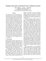
MCAT
M131
Figure 1: A subhierarchy of Reuters.
-M132
M11 -M12 M13
M14
M143 -M142 -M141
MCAT
-M131
Figure 2: A tree representing a category assignment hy-
pothesis for the subhierarchy in Fig. 1.
the SVM classification output (i.e., the example mar-
gin). Typically, a large margin corresponds to high
probability for d to be in the category whereas small
margin indicates low probability
1
. Let us indicate
with h = {h
1
, , h
n
} ∈ {0, 1}
n
a classification hy-
pothesis, i.e., the set of n binary decisions for a doc-
ument d. If we assume independence between the
SVM scores, the most probable hypothesis on d is

˜
h = argmax
h∈{0,1}
n
n

i=1
p
h
i
i
(d) =

argmax
h∈{0,1}
p
h
i
(d)

n
i=1
.
Given
˜
h, the second best hypothesis can be ob-
tained by changing the label on the least probable
classification, i.e., associated with the index j =
argmin
i=1, ,n

p
˜
h
i
i
(d). By storing the probability of the
k − 1 most probable configurations, the next k best
hypotheses can be efficiently generated.
3 Structural Kernels for Reranking
Hierarchical Classification
In this section we describe our hypothesis reranker.
The main idea is to represent the hypotheses as a
tree structure, naturally derived from the hierarchy
and then to use tree kernels to encode such a struc-
tural description in a learning algorithm. For this
purpose, we describe our hypothesis representation,
kernel methods and the kernel-based approach to
preference reranking.
3.1 Encoding hypotheses in a tree
Once hypotheses are generated, we need a represen-
tation from which the dependencies between the dif-
1
We used the conversion of margin into probability provided
by LIBSVM.
760
M11 M13
M14
M143
MCAT
Figure 3: A compact representation of the hypothesis in

Fig. 2.
ferent nodes of the hierarchy can be learned. Since
we do not know in advance which are the important
dependencies and not even the scope of the interac-
tion between the different structure subparts, we rely
on automatic feature engineering via structural ker-
nels. For this paper, we consider tree-shaped hier-
archies so that tree kernels, e.g. (Collins and Duffy,
2002; Moschitti, 2006a), can be applied.
In more detail, we focus on the Reuters catego-
rization scheme. For example, Figure 1 shows a sub-
hierarchy of the Markets (MCAT) category and its
subcategories: Equity Markets (M11), Bond Mar-
kets (M12), Money Markets (M13) and Commod-
ity Markets (M14). These also have subcategories:
Interbank Markets (M131), Forex Markets (M132),
Soft Commodities (M141), Metals Trading (M142)
and Energy Markets (M143).
As the input of our reranker, we can simply use
a tree representing the hierarchy above, marking the
negative assignments of the current hypothesis in the
node labels with “-”, e.g., -M142 means that the doc-
ument was not classified in Metals Trading. For ex-
ample, Figure 2 shows the representation of a classi-
fication hypothesis consisting in assigning the target
document to the categories MCAT, M11, M13, M14
and M143.
Another more compact representation is the hier-
archy tree from which all the nodes associated with
a negative classification decision are removed. As

only a small subset of nodes of the full hierarchy will
be positively classified the tree will be much smaller.
Figure 3 shows the compact representation of the hy-
pothesis in Fig. 2. The next sections describe how to
exploit these kinds of representations.
3.2 Structural Kernels
In kernel-based machines, both learning and classi-
fication algorithms only depend on the inner prod-
uct between instances. In several cases, this can be
efficiently and implicitly computed by kernel func-
tions by exploiting the following dual formulation:

i=1 l
y
i
α
i
φ(o
i
)φ(o) + b = 0, where o
i
and o are
two objects, φ is a mapping from the objects to fea-
ture vectors x
i
and φ(o
i
)φ(o) = K(o
i
, o) is a ker-

nel function implicitly defining such a mapping. In
case of structural kernels, K determines the shape of
the substructures describing the objects above. The
most general kind of kernels used in NLP are string
kernels, e.g. (Shawe-Taylor and Cristianini, 2004),
the Syntactic Tree Kernels (Collins and Duffy, 2002)
and the Partial Tree Kernels (Moschitti, 2006a).
3.2.1 String Kernels
The String Kernels (SK) that we consider count
the number of subsequences shared by two strings
of symbols, s
1
and s
2
. Some symbols during the
matching process can be skipped. This modifies
the weight associated with the target substrings as
shown by the following SK equation:
SK(s
1
, s
2
) =

u∈Σ
∗
φ
u
(s
1

) · φ
u
(s
2
) =

u∈Σ
∗


I
1
:u=s
1
[

I
1
]


I
2
:u=s
2
[

I
2
]

λ
d(

I
1
)+d(

I
2
)
where, Σ
∗
=

∞
n=0
Σ
n
is the set of all strings,

I
1
and

I
2
are two sequences of indexes

I = (i
1

, , i
|u|
),
with 1 ≤ i
1
< < i
|u|
≤ |s|, such that u = s
i
1
s
i
|u|
,
d(

I) = i
|u|
− i
1
+ 1 (distance between the first and
last character) and λ ∈ [0, 1] is a decay factor.
It is worth noting that: (a) longer subsequences
receive lower weights; (b) some characters can be
omitted, i.e. gaps; (c) gaps determine a weight since
the exponent of λ is the number of characters and
gaps between the first and last character; and (c)
the complexity of the SK computation is O(mnp)
(Shawe-Taylor and Cristianini, 2004), where m and
n are the lengths of the two strings, respectively and

p is the length of the largest subsequence we want to
consider.
In our case, given a hypothesis represented as
a tree like in Figure 2, we can visit it and derive
a linearization of the tree. SK applied to such
a node sequence can derive useful dependencies
between category nodes. For example, using the
Breadth First Search on the compact representa-
tion, we get the sequence [MCAT, M11, M13,
M14, M143], which generates the subsequences,
[MCAT, M11], [MCAT, M11, M13, M14],
[M11, M13, M143], [M11, M13, M143]
and so on.
761
M11 -M12 M13 M14
MCAT
M11 -M12 M13 M14
MCAT
-M132 -M131
-M132 -M131
M14
M143 -M142 -M141
M11 -M12 M13 M14
MCAT
M143 -M142 -M141
M13
Figure 4: The tree fragments of the hypothesis in Fig. 2
generated by STK
M14
-M143 -M142 -M141 -M132

M13
-M131
M11 -M12 M13 M14
MCAT
M11
MCAT
-M132
M13
-M131
M13
MCAT
-M131
-M132
M13 M14
-M142 -M141
M11 -M12 M13
MCAT
MCAT
MCAT
Figure 5: Some tree fragments of the hypothesis in Fig. 2
generated by PTK
3.2.2 Tree Kernels
Convolution Tree Kernels compute the number
of common substructures between two trees T
1
and T
2
without explicitly considering the whole
fragment space. For this purpose, let the set
F = {f

1
, f
2
, . . . , f
|F|
} be a tree fragment space and
χ
i
(n) be an indicator function, equal to 1 if the
target f
i
is rooted at node n and equal to 0 oth-
erwise. A tree-kernel function over T
1
and T
2
is
T K(T
1
, T
2
) =

n
1
∈N
T
1

n

2
∈N
T
2
∆(n
1
, n
2
), N
T
1
and N
T
2
are the sets of the T
1
’s and T
2
’s nodes,
respectively and ∆(n
1
, n
2
) =

|F|
i=1
χ
i
(n

1
)χ
i
(n
2
).
The latter is equal to the number of common frag-
ments rooted in the n
1
and n
2
nodes. The ∆ func-
tion determines the richness of the kernel space and
thus different tree kernels. Hereafter, we consider
the equation to evaluate STK and PTK.
2
Syntactic Tree Kernels (STK) To compute STK,
it is enough to compute ∆
ST K
(n
1
, n
2
) as follows
(recalling that since it is a syntactic tree kernels, each
node can be associated with a production rule): (i)
if the productions at n
1
and n
2

are different then
∆
ST K
(n
1
, n
2
) = 0; (ii) if the productions at n
1
and n
2
are the same, and n
1
and n
2
have only
leaf children then ∆
ST K
(n
1
, n
2
) = λ; and (iii) if
the productions at n
1
and n
2
are the same, and n
1
and n

2
are not pre-terminals then ∆
ST K
(n
1
, n
2
) =
λ

l(n
1
)
j=1
(1 + ∆
ST K
(c
j
n
1
, c
j
n
2
)), where l(n
1
) is the
2
To have a similarity score between 0 and 1, a normalization
in the kernel space, i.e.

T K(T
1
,T
2
)
√
T K(T
1
,T
1
)×T K(T
2
,T
2
)
is applied.
number of children of n
1
and c
j
n
is the j-th child
of the node n. Note that, since the productions
are the same, l(n
1
) = l(n
2
) and the computational
complexity of STK is O(|N
T

1
||N
T
2
|) but the aver-
age running time tends to be linear, i.e. O(|N
T
1
| +
|N
T
2
|), for natural language syntactic trees (Mos-
chitti, 2006a; Moschitti, 2006b).
Figure 4 shows the five fragments of the hypothe-
sis in Figure 2. Such fragments satisfy the constraint
that each of their nodes includes all or none of its
children. For example, [M13 [-M131 -M132]] is an
STF, which has two non-terminal symbols, -M131
and -M132, as leaves while [M13 [-M131]] is not an
STF.
The Partial Tree Kernel (PTK) The compu-
tation of PTK is carried out by the following
∆
P TK
function: if the labels of n
1
and n
2
are dif-

ferent then ∆
P TK
(n
1
, n
2
) = 0; else ∆
P TK
(n
1
, n
2
) =
µ

λ
2
+


I
1
,

I
2
,l(

I
1

)=l(

I
2
)
λ
d(

I
1
)+d(

I
2
)
l(

I
1
)

j=1
∆
P T K
(c
n
1
(

I

1j
), c
n
2
(

I
2j
))

where d(

I
1
) =

I
1l(

I
1
)
−

I
11
and d(

I
2

) =

I
2l(

I
2
)
−

I
21
. This way, we penalize both larger trees and
child subsequences with gaps. PTK is more gen-
eral than STK as if we only consider the contribu-
tion of shared subsequences containing all children
of nodes, we implement STK. The computational
complexity of PTK is O(pρ
2
|N
T
1
||N
T
2
|) (Moschitti,
2006a), where p is the largest subsequence of chil-
dren that we want consider and ρ is the maximal out-
degree observed in the two trees. However the aver-
age running time again tends to be linear for natural

language syntactic trees (Moschitti, 2006a).
Given a target T , PTK can generate any subset of
connected nodes of T , whose edges are in T . For
example, Fig. 5 shows the tree fragments from the
hypothesis of Fig. 2. Note that each fragment cap-
tures dependencies between different categories.
3.3 Preference reranker
When training a reranker model, the task of the ma-
chine learning algorithm is to learn to select the best
candidate from a given set of hypotheses. To use
SVMs for training a reranker, we applied Preference
Kernel Method (Shen et al., 2003). The reduction
method from ranking tasks to binary classification is
an active research area; see for instance (Balcan et
al., 2008) and (Ailon and Mohri, 2010).
762
Category
Child-free Child-full
Train Train1 Train2 TEST Train Train1 Train2 TEST
C152 837 370 467 438 837 370 467 438
GPOL 723 357 366 380 723 357 366 380
M11 604 309 205 311 604 309 205 311

C31 313 163 150 179 531 274 257 284
E41 191 89 95 102 223 121 102 118
GCAT 345 177 168 173 3293 1687 1506 1600

E31 11 4 7 6 32 21 11 19
M14 96 49 47 58 1175 594 581 604
G15 5 4 1 0 290 137 153 146

Total: 103 10,000 5,000 5,000 5,000 10,000 5,000 5,000 5,000
Table 1: Instance distributions of RCV1: the most populated categories are on the top, the medium sized ones follow
and the smallest ones are at the bottom. There are some difference between child-free and child-full setting since for
the former, from each node, we removed all the documents in its children.
In the Preference Kernel approach, the reranking
problem – learning to pick the correct candidate h
1
from a candidate set {h
1
, . . . , h
k
} – is reduced to a
binary classification problem by creating pairs: pos-
itive training instances h
1
, h
2
, . . . , h
1
, h
k
 and
negative instances h
2
, h
1
, . . . , h
k
, h
1

. This train-
ing set can then be used to train a binary classifier.
At classification time, pairs are not formed (since the
correct candidate is not known); instead, the stan-
dard one-versus-all binarization method is still ap-
plied.
The kernels are then engineered to implicitly
represent the differences between the objects in
the pairs. If we have a valid kernel K over the
candidate space T , we can construct a preference
kernel P
K
over the space of pairs T × T as follows:
P
K
(x, y) =
P
K
(x
1
, x
2
, y
1
, y
2
) = K(x
1
, y
1

)+
K(x
2
, y
2
) − K(x
1
, y
2
) − K(x
2
, y
1
),
(1)
where x, y ∈ T × T . It is easy to show (Shen et al.,
2003) that P
K
is also a valid Mercer’s kernel. This
makes it possible to use kernel methods to train the
reranker.
We explore innovative kernels K to be used in
Eq. 1:
K
J
= p(x
1
) × p(y
1
) + S, where p(·) is the global

joint probability of a target hypothesis and S is
a structural kernel, i.e., SK, STK and PTK.
K
P
= x
1
· y
1
+ S, where x
1
={p(x
1
, j)}
j∈x
1
,
y
1
= {p(y
1
, j)}
j∈y
1
, p(t, n) is the classifica-
tion probability of the node (category) n in the
F 1 BL BOL SK STK PTK
Micro-F
1
0.769 0.771 0.786 0.790 0.790
Macro-F

1
0.539 0.541 0.542 0.547 0.560
Table 2: Comparison of rerankers using different kernels,
child-full setting (K
J
model).
F 1 BL BOL SK STK PTK
Micro-F
1
0.640 0.649 0.653 0.677 0.682
Macro-F
1
0.408 0.417 0.431 0.447 0.447
Table 3: Comparison of rerankers using different kernels,
child-free setting (K
J
model).
tree t ∈ T and S is again a structural kernel,
i.e., SK, STK and PTK.
For comparative purposes, we also use for S a lin-
ear kernel over the bag-of-labels (BOL). This is
supposed to capture non-structural dependencies be-
tween the category labels.
4 Experiments
The aim of the experiments is to demonstrate that
our reranking approach can introduce semantic de-
pendencies in the hierarchical classification model,
which can improve accuracy. For this purpose, we
show that several reranking models based on tree
kernels improve the classification based on the flat

one-vs all approach. Then, we analyze the effi-
ciency of our models, demonstrating their applica-
bility.
4.1 Setup
We used two full hierarchies, TOPICS and INDUS-
TRY of Reuters Corpus Volume 1 (RCV1)
3
TC cor-
3
trec.nist.gov/data/reuters/reuters.html
763
pus. For most experiments, we randomly selected
two subsets of 10k and 5k of documents for train-
ing and testing from the total 804,414 Reuters news
from TOPICS by still using all the 103 categories
organized in 5 levels (hereafter SAM). The distri-
bution of the data instances of some of the dif-
ferent categories in such samples can be observed
in Table 1. The training set is used for learning
the binary classifiers needed to build the multiclass-
classifier (MCC). To compare with previous work
we also considered the Lewis’ split (Lewis et al.,
2004), which includes 23,149 news for training and
781,265 for testing.
Additionally, we carried out some experiments on
INDUSTRY data from RCV1. This contains 352,361
news assigned to 365 categories, which are orga-
nized in 6 levels. The Lewis’ split for INDUSTRY in-
cludes 9,644 news for training and 342,117 for test-
ing. We used the above datasets with two different

settings: the child-free setting, where we removed
all the document belonging to the child nodes from
the parent nodes, and the normal setting which we
refer to as child-full.
To implement the baseline model, we applied the
state-of-the-art method used by (Lewis et al., 2004)
for RCV1, i.e.,: SVMs with the default parameters
(trade-off and cost factor = 1), linear kernel, normal-
ized vectors, stemmed bag-of-words representation,
log(T F + 1) × IDF weighting scheme and stop
list
4
. We used the LIBSVM
5
implementation, which
provides a probabilistic outcome for the classifica-
tion function. The classifiers are combined using the
one-vs all approach, which is also state-of-the-art
as argued in (Rifkin and Klautau, 2004). Since the
task requires us to assign multiple labels, we simply
collect the decisions of the n classifiers: this consti-
tutes our MCC baseline.
Regarding the reranker, we divided the training
set in two chunks of data: Train1 and Train2. The
binary classifiers are trained on Train1 and tested on
Train2 (and vice versa) to generate the hypotheses
on Train2 (Train1). The union of the two sets con-
stitutes the training data for the reranker. We imple-
4
We have just a small difference in the number of tokens,

i.e., 51,002 vs. 47,219 but this is both not critical and rarely
achievable because of the diverse stop lists or tokenizers.
5
/>˜
cjlin/
libsvm/
0.626
0.636
0.646
0.656
0.666
0.676
2 7 12 17 22 27 32
Micro-F1
Training Data Size (thousands of instances)
BL (Child-free)
RR (Child-free)
FRR (Child-free)
Figure 6: Learning curves of the reranking models using
STK in terms of MicroAverage-F1, according to increas-
ing training set (child-free setting).
0.365
0.375
0.385
0.395
0.405
0.415
0.425
0.435
0.445

2 7 12 17 22 27 32
Macro-F1
Training Data Size (thousands of instances)
BL (Child-free)
RR (Child-free)
FRR (Child-free)
Figure 7: Learning curves of the reranking models using
STK in terms of MacroAverage-F1, according to increas-
ing training set (child-free setting).
mented two rerankers: RR, which use the represen-
tation of hypotheses described in Fig. 2; and FRR,
i.e., fast RR, which uses the compact representation
described in Fig. 3.
The rerankers are based on SVMs and the Prefer-
ence Kernel (P
K
) described in Sec. 1 built on top of
SK, STK or PTK (see Section 3.2.2). These are ap-
plied to the tree-structured hypotheses. We trained
the rerankers using SVM-light-TK
6
, which enables
the use of structural kernels in SVM-light (Joachims,
1999). This allows for applying kernels to pairs of
trees and combining them with vector-based kernels.
Again we use default parameters to facilitate replica-
bility and preserve generality. The rerankers always
use 8 best hypotheses.
All the performance values are provided by means
of Micro- and Macro-Average F1, evaluated on test

6
disi.unitn.it/moschitti/Tree-Kernel.htm
764
Cat.
Child-free Child-full
BL K
J
K
P
BL K
J
K
P
C152 0.671 0.700 0.771 0.671 0.729 0.745
GPOL 0.660 0.695 0.743 0.660 0.680 0.734
M11 0.851 0.891 0.901 0.851 0.886 0.898

C31 0.225 0.311 0.446 0.356 0.421 0.526
E41 0.643 0.714 0.719 0.776 0.791 0.806
GCAT 0.896 0.908 0.917 0.908 0.916 0.926

E31 0.444 0.600 0.600 0.667 0.765 0.688
M14 0.591 0.600 0.575 0.887 0.897 0.904
G15 0.250 0.222 0.250 0.823 0.806 0.826
103 cat.
Mi-F1 0.640 0.677 0.731 0.769 0.794 0.815
Ma-F1 0.408 0.447 0.507 0.539 0.567 0.590
Table 4: F1 of some binary classifiers along with the
Micro and Macro-Average F1 over all 103 categories
of RCV1, 8 hypotheses and 32k of training data for

rerankers using STK.
data over all categories (103 or 363). Additionally,
the F1 of some binary classifiers are reported.
4.2 Classification Accuracy
In the first experiments, we compared the different
kernels using the K
J
combination (which exploits
the joint hypothesis probability, see Sec. 3.3) on
SAM. Tab. 2 shows that the baseline (state-of-the-
art flat model) is largely improved by all rerankers.
BOL cannot capture the same dependencies as the
structural kernels. In contrast, when we remove the
dependencies generated by shared documents be-
tween a node and its descendants (child-free setting)
BOL improves on BL. Very interestingly, TK and
PTK in this setting significantly improves on SK
suggesting that the hierarchical structure is more im-
portant than the sequential one.
To study how much data is needed for the
reranker, the figures 6 and 7 report the Micro and
Macro Average F1 of our rerankers over 103 cate-
gories, according to different sets of training data.
This time, K
J
is applied to only STK. We note that
(i) a few thousands of training examples are enough
to deliver most of the RR improvement; and (ii) the
FRR produces similar results as standard RR. This is
very interesting since, as it will be shown in the next

section, the compact representation produces much
faster models.
Table 4 reports the F1 of some individual cate-
gories as well as global performance. In these exper-
iments we used STK in K
J
and K
P
. We note that
0
50
100
150
200
250
300
350
400
450
2 12 22 32 42 52 62
Time (min)
Training Data Size (thousands of instances)
RR trainingTime
RR testTime
FRR trainingTime
FRR testTime
Figure 8: Training and test time of the rerankers trained
on data of increasing size.
K
P

highly improves on the baseline on child-free
setting by about 7.1 and 9.9 absolute percent points
in Micro-and Macro-F1, respectively. Also the im-
provement on child-full is meaningful, i.e., 4.6 per-
cent points. This is rather interesting as BOL (not
reported in the table) achieved a Micro-average of
80.4% and a Macro-average of 57.2% when used in
K
P
, i.e., up to 2 points below STK. This means that
the use of probability vectors and combination with
structural kernels is a very promising direction for
reranker design.
To definitely assess the benefit of our rerankers
we tested them on the Lewis’ split of two different
datasets of RCV1, i.e., TOPIC and INDUSTRY. Ta-
ble 5 shows impressive results, e.g., for INDUSTRY,
the improvement is up to 5.2 percent points. We car-
ried out statistical significance tests, which certified
the significance at 99%. This was expected as the
size of the Lewis’ test sets is in the order of several
hundreds thousands.
Finally, to better understand the potential of
reranking, Table 6 shows the oracle performance
with respect to the increasing number of hypothe-
ses. The outcome clearly demonstrates that there is
large margin of improvement for the rerankers.
4.3 Running Time
To study the applicability of our rerankers, we have
analyzed both the training and classification time.

Figure 8 shows the minutes required to train the dif-
ferent models as well as to classify the test set ac-
cording to data of increasing size.
It can be noted that the models using the compact
hypothesis representation are much faster than those
765
F1
Topic Industry
BL (Lewis) BL (Ours) K
J
(BOL) K
J
K
P
BL (Lewis) BL (Ours) K
J
(BOL) K
J
K
P
Micro-F1 0.816 0.815 0.818 0.827 0.849 0.512 0.562 0.566 0.576 0.628
Macro-F1 0.567 0.566 0.571 0.590 0.615 0.263 0.289 0.243 0.314 0.341
Table 5: Comparison between rankers using STK or BOL (when indicated) with the K
J
and K
P
schema. 32k
examples are used for training the rerankers with child-full setting.
k Micro-F
1

Macro-F
1
1 0.640 0.408
2 0.758 0.504
4 0.821 0.566
8 0.858 0.610
16 0.898 0.658
Table 6: Oracle performance according to the number of
hypotheses (child-free setting).
using the complete hierarchy as representation, i.e.,
up to five times in training and eight time in test-
ing. This is not surprising as, in the latter case,
each kernel evaluation requires to perform tree ker-
nel evaluation on trees of 103 nodes. When using
the compact representation the number of nodes is
upper-bounded by the maximum number of labels
per documents, i.e., 6, times the depth of the hierar-
chy, i.e., 5 (the positive classification on the leaves
is the worst case). Thus, the largest tree would con-
tain 30 nodes. However, we only have 1.82 labels
per document on average, therefore the trees have
an average size of only about 9 nodes.
5 Related Work
Tree and sequence kernels have been successfully
used in many NLP applications, e.g.: parse rerank-
ing and adaptation (Collins and Duffy, 2002; Shen
et al., 2003; Toutanova et al., 2004; Kudo et al.,
2005; Titov and Henderson, 2006), chunking and
dependency parsing (Kudo and Matsumoto, 2003;
Daum

´
e III and Marcu, 2004), named entity recog-
nition (Cumby and Roth, 2003), text categorization
(Cancedda et al., 2003; Gliozzo et al., 2005) and re-
lation extraction (Zelenko et al., 2002; Bunescu and
Mooney, 2005; Zhang et al., 2006).
To our knowledge, ours is the first work explor-
ing structural kernels for reranking hierarchical text
categorization hypotheses. Additionally, there is a
substantial lack of work exploring reranking for hi-
erarchical text categorization. The work mostly re-
lated to ours is (Rousu et al., 2006) as they directly
encoded global dependencies in a gradient descen-
dent learning approach. This kind of algorithm is
less efficient than ours so they could experiment
with only the CCAT subhierarchy of RCV1, which
only contains 34 nodes. Other relevant work such
as (McCallum et al., 1998) and (Dumais and Chen,
2000) uses a rather different datasets and a different
idea of dependencies based on feature distributions
over the linked categories. An interesting method is
SVM-struct (Tsochantaridis et al., 2005), which has
been applied to model dependencies expressed as
category label subsets of flat categorization schemes
but no solution has been attempted for hierarchical
settings. The approaches in (Finley and Joachims,
2007; Riezler and Vasserman, 2010; Lavergne et al.,
2010) can surely be applied to model dependencies
in a tree, however, they need that feature templates
are specified in advance, thus the meaningful depen-

dencies must be already known. In contrast, kernel
methods allow for automatically generating all pos-
sible dependencies and reranking can efficiently en-
code them.
6 Conclusions
In this paper, we have described several models for
reranking the output of an MCC based on SVMs
and structural kernels, i.e., SK, STK and PTK.
We have proposed a simple and efficient algorithm
for hypothesis generation and their kernel-based
representations. The latter are exploited by SVMs
using preference kernels to automatically derive
features from the hypotheses. When using tree
kernels such features are tree fragments, which can
encode complex semantic dependencies between
categories. We tested our rerankers on the entire
well-known RCV1. The results show impressive
improvement on the state-of-the-art flat TC models,
i.e., 3.3 absolute percent points on the Lewis’ split
(same setting) and up to 10 absolute points on
samples using child-free setting.
Acknowledgements This research is partially sup-
ported by the EC FP7/2007-2013 under the grants:
247758 (ETERNALS), 288024 (LIMOSINE) and 231126
(LIVINGKNOWLEDGE). Many thanks to the reviewers
for their valuable suggestions.
766
References
Nir Ailon and Mehryar Mohri. 2010. Preference-based
learning to rank. Machine Learning.

Maria-Florina Balcan, Nikhil Bansal, Alina Beygelzimer,
Don Coppersmith, John Langford, and Gregory B.
Sorkin. 2008. Robust reductions from ranking to clas-
sification. Machine Learning, 72(1-2):139–153.
Razvan Bunescu and Raymond Mooney. 2005. A short-
est path dependency kernel for relation extraction. In
Proceedings of HLT and EMNLP, pages 724–731,
Vancouver, British Columbia, Canada, October.
Nicola Cancedda, Eric Gaussier, Cyril Goutte, and
Jean Michel Renders. 2003. Word sequence kernels.
Journal of Machine Learning Research, 3:1059–1082.
Michael Collins and Nigel Duffy. 2002. New ranking
algorithms for parsing and tagging: Kernels over dis-
crete structures, and the voted perceptron. In Proceed-
ings of ACL’02, pages 263–270.
Chad Cumby and Dan Roth. 2003. On kernel methods
for relational learning. In Proceedings of ICML 2003.
Hal Daum
´
e III and Daniel Marcu. 2004. Np bracketing
by maximum entropy tagging and SVM reranking. In
Proceedings of EMNLP’04.
Susan T. Dumais and Hao Chen. 2000. Hierarchical clas-
sification of web content. In Nicholas J. Belkin, Peter
Ingwersen, and Mun-Kew Leong, editors, Proceedings
of SIGIR-00, 23rd ACM International Conference on
Research and Development in Information Retrieval,
pages 256–263, Athens, GR. ACM Press, New York,
US.
T. Finley and T. Joachims. 2007. Parameter learning

for loopy markov random fields with structural support
vector machines. In ICML Workshop on Constrained
Optimization and Structured Output Spaces.
Alfio Gliozzo, Claudio Giuliano, and Carlo Strapparava.
2005. Domain kernels for word sense disambiguation.
In Proceedings of ACL’05, pages 403–410.
Thorsten Joachims. 1999. Making large-scale SVM
learning practical. Advances in Kernel Methods – Sup-
port Vector Learning, 13.
Taku Kudo and Yuji Matsumoto. 2003. Fast methods for
kernel-based text analysis. In Proceedings of ACL’03.
Taku Kudo, Jun Suzuki, and Hideki Isozaki. 2005.
Boosting-based parse reranking with subtree features.
In Proceedings of ACL’05.
T. Lavergne, O. Capp
´
e, and F. Yvon. 2010. Practical very
large scale CRFs. In Proc. of ACL, pages 504–513.
D. D. Lewis, Y. Yang, T. Rose, and F. Li. 2004. Rcv1: A
new benchmark collection for text categorization re-
search. The Journal of Machine Learning Research,
(5):361–397.
Andrew McCallum, Ronald Rosenfeld, Tom M. Mitchell,
and Andrew Y. Ng. 1998. Improving text classifica-
tion by shrinkage in a hierarchy of classes. In ICML,
pages 359–367.
Alessandro Moschitti. 2006a. Efficient convolution ker-
nels for dependency and constituent syntactic trees. In
Proceedings of ECML’06.
Alessandro Moschitti. 2006b. Making tree kernels prac-

tical for natural language learning. In Proccedings of
EACL’06.
S. Riezler and A. Vasserman. 2010. Incremental feature
selection and l1 regularization for relaxed maximum-
entropy modeling. In EMNLP.
Ryan Rifkin and Aldebaro Klautau. 2004. In defense of
one-vs-all classification. J. Mach. Learn. Res., 5:101–
141, December.
Juho Rousu, Craig Saunders, Sandor Szedmak, and John
Shawe-Taylor. 2006. Kernel-based learning of hierar-
chical multilabel classification models. The Journal of
Machine Learning Research, (7):1601–1626.
John Shawe-Taylor and Nello Cristianini. 2004. Kernel
Methods for Pattern Analysis. Cambridge University
Press.
Libin Shen, Anoop Sarkar, and Aravind k. Joshi. 2003.
Using LTAG Based Features in Parse Reranking. In
Empirical Methods for Natural Language Processing
(EMNLP), pages 89–96, Sapporo, Japan.
Ivan Titov and James Henderson. 2006. Porting statisti-
cal parsers with data-defined kernels. In Proceedings
of CoNLL-X.
Kristina Toutanova, Penka Markova, and Christopher
Manning. 2004. The Leaf Path Projection View of
Parse Trees: Exploring String Kernels for HPSG Parse
Selection. In Proceedings of EMNLP 2004.
Ioannis Tsochantaridis, Thorsten Joachims, Thomas Hof-
mann, and Yasemin Altun. 2005. Large margin
methods for structured and interdependent output vari-
ables. J. Machine Learning Reserach., 6:1453–1484,

December.
Dmitry Zelenko, Chinatsu Aone, and Anthony
Richardella. 2002. Kernel methods for relation
extraction. In Proceedings of EMNLP-ACL, pages
181–201.
Min Zhang, Jie Zhang, and Jian Su. 2006. Explor-
ing Syntactic Features for Relation Extraction using a
Convolution tree kernel. In Proceedings of NAACL.
767