Dynamical analysis of a predator-prey model using hunting strategies

TNU Journal of Science and Technology

227(15): 47 -57

DYNAMICAL ANALYSIS OF A PREDATOR - PREY MODEL
USING HUNTING STRATEGIES
Ha Thi Ngoc Yen*, Nguyen Phuong Thuy
School of Applied Mathematics and Informatics, Hanoi University of Science and Technology

ARTICLE INFO
Received:

11/8/2022

Revised:

22/8/2022

Published:

24/8/2022

KEYWORDS
Prey-predator model
Aggregated method
Game theory
Hunting strategy
Stability analysis

ABSTRACT
In this paper, we establish a new prey-predator model using game

theory with solitary hunting or pack hunting strategies. The model
includes a fast-time scale and a slow-time scale to investigate the effect
of predator behavior on the ecosystem. In our model, we assume that
the switch between hunting strategies and hawk-dove tactics happens
on a fast-time scale, while the development of the species of prey
intrinsic growth, predator mortality, and hunting process, takes place on
a slow-time scale. We use the differential equations theory and the
aggregated method to study the model’s well-posedness and the
properties of its solution, such as positivity, boundedness, and stability.
It is shown that the coexistence of prey and predator might be in a
steady state or a chaotic state. Some numerical simulations illustrate the
theoretical results in cases of stable equilibrium and chaotic equilibrium
are given. Discussions about predators' behavior and the ecosystem's
development are also provided.

PHÂN TÍCH HỆ ĐỘNG LỰC THÚ MỒI SỬ DỤNG CHIẾN THUẬT SĂN MỒI
Hà Thị Ngọc Yến*, Nguyễn Phương Thuỳ
Viện Toán ứng dụng và Tin học, Trường Đại học Bách khoa Hà Nội

THÔNG TIN BÀI BÁO
Ngày nhận bài:

11/8/2022

Ngày hồn thiện:

22/8/2022

Ngày đăng:

24/8/2022

TỪ KHĨA
Mơ hình thú mồi
Phương pháp tổ hợp biến
Lý thuyết trò chơi
Chiến thuật săn mồi
Phân tích ổn định

TĨM TẮT
Trong bài báo này, chúng tơi xây dựng một mơ hình thú mồi mới với
tập tính săn mồi theo bầy đàn hoặc đơn lẻ sử dụng lý thuyết trị chơi.
Mơ hình bao gồm hai thang thời gian nhanh và chậm nhằm khảo sát ảnh
hưởng của hành vi săn mồi đối với hệ sinh thái. Giả sử rằng, sự chuyển
đổi chiến thuật săn mồi diễn ra trên thang thời gian nhanh và sự phát
triển loài như q trình tăng trưởng nội tại của lồi mồi, q trình chết
tự nhiên của lồi thú và q trình săn bắt mồi được xét trên thang thời
gian chậm. Lý thuyết phương trình vi phân và phương pháp tổ hợp biến
được sử dụng để khảo sát tính đặt chỉnh và một số tính chất định tính
của nghiệm bài tốn như tính chất dương, tính bị chặn, tính chất ổn
định. Các phân tích hệ động lực chỉ ra rằng, sự sinh tồn đồng thời của
hai lồi có thể đạt trạng thái ổn định hoặc trạng thái hỗn loạn. Chúng tôi
mô phỏng số cho mơ hình, minh hoạ trường hợp điểm cân bằng ổn định
và điểm cân bằng hỗn loạn. Trên cơ sở đó, một số bình luận về hành vi
của lồi thú và sự phát triển của hệ sinh thái đã được đưa ra.

DOI: />*

Corresponding author. Email:

47

Email:


TNU Journal of Science and Technology

227(15): 47 - 57

1. Introduction
Biological population dynamics is very attractive to most of mathematical biologists. There are different
ways to explore the population dynamics. Evolutionary game theory is one of the most useful ways in
studying the dynamics involving the behavior of the objects. In 1973, an application of game theory in
exploring the biological evolution is first introduced by John Maynard Smith and George Robert Price
[1]. John Maynard Smith introduced his work on theory of evolutionary stable strategy (ESS) in his book
”Evolution and the Theory of Games” [2]. ESS becomes familiar to scientists [3],[4].
The combination of predator - prey model and game theory is effectively used to explore the effect of
predator behavior on the dynamics. Since 1998, Auger et al. have presented some results on the predatorprey models with the hawk - dove game (aka the chicken game) [5]–[7]. A model with N-person hawk dove games which considered the fighting between N hawks for food was studied in [8] by Wei Chen et al.
Recently, some results on predator - prey model using Rock-Paper-Scissor strategies have been established
[9]–[11].
In this paper, we study a predator-prey model combining the classical model in slow time scale as in
[6] with the changing behavior of predator following the chicken game in fast time scale. We consider a
predator and prey model in which the predator uses hawk-dove tactics in combination with solitary hunting
or pack hunting behavior. There is a lack of research on this problem till now.
The model in this paper includes population of prey, population of predator, behavior of predator in
catching prey: in group or alone, aggressive or not. In fact, when predators see the same prey at the same
time, they might cooperate with the others to fight for food or retreat to avoid fighting. Which tactics in
which conditions would be more beneficial? That is the reason why we are interested in exploring the

model with the different behaviors of the predator.
The rest of this paper is organized as follows: In Section 2, the mathematical model with ecological
assumptions and the meaning of parameters are described. Section 3 derives the positivity and the boundedness of solutions and presents the aggregation model. In Section 4, the stability analysis of the equilibrium
points is presented. Section 5 is devoted to the illustration of some numerical simulations of our theoretical results. Finally, we give some discussions and the biological significance of our analytical findings in
Section 6.
2. Model formulation
Let t and τ be the notations of time on slow and fast time scale, respectively. We denote n(t) and p(t)
as the densities of the prey and predator, respectively, at time t. We shall build up a model describing what
happens on both time scales: the changes of predation strategies on the fast time scale, and the hunting
process and development of the species on the slow one.
2.1. Hunting game dynamics on the fast time scale
At first, we will introduce the rules of the hunting game. Assuming that at time t, predators are divided
into two sub-groups, named the pack predators and the solitary predators. The pack group includes all
predators that choose to cooperate with the others to fight for food. The solitary group includes all predators
that choose to independently fight another single or to retreat to avoid combat. Let denote pA (t) and pL (t)
as the pack predator and solitary predator densities, respectively, at time t. The total density of predators
is given by
p(t) = pA (t) + pL (t).
(1)
On the fast time scale, predators fight for a captured prey. During an encounter, one individual must choose
either to cooperate with the others in a herd or to hunt independently. Furthermore, we assume that
herds have the same size and let q ≥ 2 is the number of the individuals of one. The game describes this
process of conflicts between two predation herds and between two single predators. The gain G of the game
corresponds to the prey amount that the predators dispute over during each unit of time. In this model, we
assume that the amount of prey killed per unit of time per one predator is proportional to the density of
prey with a proportional coefficient a > 0. In other words, the gain G(n) of the game is the amount of prey
killed which is defined as follow:
G(n) = an.
(2)
Let C > 0 be the cost due to fighting between herds and between individuals.

Now, we denote A, L for pack group and solitary group, respectively; a coefficient Mlk of the payoff
matrix corresponds to the gain that is obtained by an individual playing tactic l against an individual playing
tactic k; l, k ∈ {A, L}. We assume that the average gain and the average cost due to injuries are equally
G −C
G −C
divided by the individuals that have the same tactic, MAA =
and MLL =
. When one individual
2q
2



48

Email:


TNU Journal of Science and Technology

227(15): 47-57

meets a herd, it always retreats and lets the group obtains the gain, which means MLA = 0, MAL =
Therefore, the payoff matrix M of the game is the following one:


G −C
G
 2q
q 



M=
.

G −C 
0
2

G
.
q

(3)

Let x and y be the proportion of pack predators and solitary ones in the total predators.
x=

pA
pL
, y=
= 1 − x.
p
p

(4)

Thus, at time t, the gain ∆A of an individual that always choose to cooperate with the others and the gain
∆L of one always choose to be single are given:
x

∆A = (1

0) M

x
and ∆L = (0

1) M

y

.

(5)

y

Therefore, the average gain of an individual playing the two tactics in proportions x and y is the following
one:
x
∆ = (x y) M
.
(6)
y
Naturally, a predator individual would choose a tactic that helps it get more benefit. It means that if the gain
for one tactic is greater (or smaller) than the average gain, the size of that tactic group should be increased
(or decreased). In additional, we assume that the game is fast in comparison to other processes. With these
assumptions, the equations for the tactic groups are given:
d pk
= pk (∆k − ∆) ,

dτ

k ∈ {A, L}.

(7)

In the next part, we shall consider processes happen on slow time scale such as the predator mortality, prey
growth and process of prey capturing.
2.2. Dynamics of prey density on the slow time scale
In the model, we assume that the intrinsic growth of prey population follows logistic function with
a natural growth rate r and an environmental carrying capacity constant K. The density of preys also
depends on the number of preys killed by predators, which is proportional to the size of prey population
and predator population. Specifically, we use a Lotka - Volterra functional response type I with the intake
rate a mentioned before in the gain G of game. Thus, the equation for the dynamics of prey is given as
follows:
dn
n
= rn 1 −
− anp,
(8)
dt
K
where t corresponds to the slow time scale. The relationship between the two time - scales is t = ετ.
2.3. Dynamics of predator densities on the slow time scale
For predators, we assume that the growth depends on only the number of preys killed. That means
predators grow by preys they catch and naturally die with mortality rate µ > 0. We also assume that each
tactic group as a proportion of predators is governed by the same rules. That leads to the following equation:
d pk
= −µ pk + α∆k pk , k ∈ {A, L}.
(9)

dt
in which α > 0 is a conversion constant of gain into biomass of predators. In other words, the growth
rate of each subgroup is proportional to the average payoff obtained by an individual in that subgroup. A
pack predator individual can encounter either another one in different herd in proportion x and gets the



49

Email:


TNU Journal of Science and Technology

227(15): 47-57

G −C
G
, or a single individual in proportion y, gets . Consequently, the growth of the pack predator
2q
q
sub-population obeys the following equation:
gain

d pA
= −µ pA + α (1
dt

x
pA = −µ pA + α

0) M
y

G −C pA G pL
. + .
2q
p
q p

pA .

(10)

Similarly, we obtain an equation that rules the population of the solitary predator subgroup with notice
that a single predator will retreat when it meets a group, gets no gain, and will equally share the gain and
cost when it meets other solitary individual.
d pL
= −µ pL + α (0
dt

x
pL = −µ pL + α

1) M
y

G −C pL
.
2

p

pL .

(11)

The predator population and prey population growths are assumed to be on slow time scale. This is matched
with the fact that the fighting between predators frequently happens while the number of preys captured
each day is much smaller than the population.
2.4. The complete slow-fast model
The complete model that combines all processes in slow and fast time scale reads as:

dn
n



ε dt = ε rn 1 − K − an(pA + pL )
(12)



ε d pk = pk (∆k − ∆) + ε [−µ pk + α∆k pk ] ,
dt
where ε

k ∈ {A, L}

1 is a small parameter. We also use the fast time scale τ to rewrite the complete model (12):


dn
n


= ε rn 1 −
− an(pA + pL )


dτ
K






 d pA
G −C pA G pL
= pA (∆A − ∆) + ε −µ pA + α
. + .
pA
(13)
dτ
2q
p
q p









d pL
G −C pL


= pL (∆L − ∆) + ε −µ pL + α
.
pL

dτ
2
p

The model (13) clearly shows that the population of prey as well as predator population change very little in
fast time scale when ε is small enough. The game dynamics on fast time scale shows the changes in the sizes
of the two tactical groups. This model is a three-dimensional system of ordinary differential equations.
3. Positivity, boundedness and aggregated model
3.1. Positivity and boundedness
In this part, we get some properties for the solutions of the complete model system (13) which relate
to the positivity and boundedness.
Theorem 0.1. All the solutions of the complete model (13), which start in R3+ are always positive and bounded.
Theorem 0.2. For any given initial value in R3+ , the complete model (13) has a unique positive solution.
These properties guarantee the meaning of exploring the model because of the positivity and boundedness of populations of prey and predators.
3.2. The aggregated model
We shall use the aggregation method, referred to [5],[12],[13], to reduce the dimension of the complete
system (13) of the three equations into the aggregated model of the two equations.
3.2.1. Fast equilibrium

50

Email:


TNU Journal of Science and Technology

227(15): 47-57

The first step of the method is to neglect the small terms O(ε) and to look for the existence of a stable
equilibrium of the game dynamics which happen on fast time scale.
d pk
= px (∆k − ∆) , k ∈ {A, L}
dτ

(14)

On fast time scale, the densities of the prey and the predator, n and p = pA + pL respectively, can be considered as constants. Moreover, because x, y are proportion of pack predator subgroup and solitary predator
subgroup in total predators, which means x + y = 1, we can reduce the system (14) of the two dimension
to one equation that rules the pack predator group. Hence, the game dynamics is ruled by the following
equation:
dx
G −C G G −C
G G −C
= x(1 − x)
− +
x+ −

.
(15)
dt
2q
q
2
q
2
The equation (15) has three equilibria of 0, 1, and x∗ =

(q − 2)G − qC
. We now consider the cases as
(q − 1)G − (q + 1)C

follows:
Case A. q > 2 ⇒ C <

q+1
qC
C<
.
q−1
q−2

According to parameters values, three cases can occur:
qC
⇒ 0 < x∗ < 1. 0, 1 are stable; and x∗ is unstable.
q−2
qC
A2. C < G <

⇒ x∗ ∈
/ [0; 1]. 1 is stable; 0 is unstable.
q−2
A1. G >

A3. G < C ⇒ x∗ ∈ [0, 1]. x∗ is stable; 0, 1 are unstable.
Case B. q = 2 ⇒ x∗ =

−2C
. We have three cases as follows:
G − 3C

B1. G > 3C ⇒ x∗ < 0 ⇒ x∗ ∈
/ [0; 1]. 1 is stable; 0 is unstable.
B2. C < G < 3C ⇒ x∗ > 1 ⇒ x∗ ∈
/ [0; 1]. 1 is stable; 0 is unstable.
B3. G < C ⇒ 0 < x∗ < 1. x∗ is stable; 0;1 are unstable.
3.2.2 Aggregated model
The second step of the aggregation method is to substitute the fast equilibrium and add the two predator
equations in the complete model with the assumption that the fast process is at the fast equilibrium. Thus,
with the notations x¯ for the stable equilibrium, p¯k , ∆¯ k , k ∈ {A, L} respectively stand for pk , ∆k , k ∈ {A, L}
at the stable equilibrium, we have the aggregated model

dn
n



 dt = n r 1 − K − ap
(16)



d
p


= − µ + α ∆¯ A x¯ + ∆¯ L (1 − x)
¯ p.
dt
We have three fast equilibria and the gain depends on the prey density G = an. Therefore, we obtain three
aggregated models which are valid on three different domains of phase plane.
• Case A, q > 2.
Model I: n >

q C
,
q−2 a

x¯ = 0 is stable in Eq. (15),
 dn
n

= n r 1−
− ap


 dt
K
(17)



dp
an −C


= −µ + α
dt
2



51

p.

Email:


TNU Journal of Science and Technology

Model II: n >

C
,
a

227(15): 47-57

x¯ = 1 is stable in Eq. (15),
 dn

n

= n r 1−
− ap


 dt
K
(18)


dp
G −C


= −µ + α
dt
2q

C
,
a

Model III: n <

p

x¯ = x∗ is stable in Eq. (15),

dn

n


 dt = n r 1 − K − ap

(19)


dp αp
1


=
.
.H(n)
dt
2 (q − 1)an − (q + 1)C

in which H(n) = a2 n2 −

2µ(q − 1)
2µ(q + 1)C
+ 2C an +
+C2 .
α
α

qC
, we have two models, namely systems (17) and (18). If x < x∗ , the model I,
(q − 2)a

Eq. (17) is governing and if x > x∗ , the model II, Eq. (18) is ruling.

When n >

• Case B, q = 2.
C
C
When n > , x¯ = 1 is stable in Eq. (15), model II, Eq. (18) is governing. When n < , x¯ = x∗ is
a
a
stable in Eq. (15), model III, Eq. (19) is ruling.
In general, there are two cases as follows:
• Case 1: Model III is valid on n, n <

C
a

. Model II is valid on n, n >

n, n <

C
a

. Model II is valid on

• Case 2: Model III is valid on
I is valid on

n, n >

n,

C
a

.

C
qC
. And Model
a
(q − 2)a

qC
.
(q − 2)a

C
In the phase space (n, p), besides the vertical line n = at which these models connect in both cases, in
a
qC
case 2, the other connected line is n =
.
(q − 2)a
4. Stability analysis of the aggregated model
The first equation of the three models are the same. That leads to the same n− nullclines: n = 0 and
r
n

p=
1−
. The p− nullclines which depend on parameters values can be found from the equations
a
K
dp
= 0 of the three models. For model I, system (17), we have two nullclines, p = 0 and the vertical line
dt
2µ + αC
dp
n = n∗1 =
. For model II, Eq. (18), there are two
= 0 nullclines, p = 0 and the vertical line
αa
dt
2µq
+
αC
n = n∗2 =
. For model III, system (19), if µ(q − 1)2 − 4αC < 0 then p = 0 is the only p− nullcline
αa
and if µ(q − 1)2 − 4αC > 0 then there are three nullclines p = 0; n = n∗3 ; n = n∗4 , where
n = n∗3;4 =



αC + µ(q − 1) ±

52

µ 2 (q − 1)2 − 4α µC
.
αa

Email:


TNU Journal of Science and Technology

227(15): 47-57

C
C
< n∗3 < n∗4 < n∗2 , and
< n∗1 < n∗2 . Thus, n∗2 is always in
a
a
the domain of model II, Eq. (18) while n∗3 , n∗4 are always not in the domain of model III, Eq. (19). In case 1,
qC
q > 2, n∗1 is in the domain of model I, system (17), if n∗1 >
. There are up to six equilibria. Two of them,
q−2
r
n∗
(0, 0); (K; 0) always exist and four others (n∗i , p∗i ), i ∈ {1; 2; 3; 4} where p∗i =
1 − i can be found in
a
K
positive quadrant if n∗i < K. In any cases, (0, 0) is a saddle point.
Those vertical nullclines are ordered as follows:

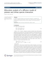
According to the position of K with respect to the other equilibria as well as the connected lines, in
each case, it is divided into some sub-cases.
C
Case 1: Fig. 1(a) corresponds to the sub-case K < , the equilibrium (K, 0) is asymptotically stable which
a
mean that the predator gets extinct, the prey tends to its carrying capacity. Fig. 1(b) corresponds to the
C
sub-case < K < n∗2 , the equilibrium (K, 0) is a stable node, the prey tends to its carrying capacity, the
a
C
predator dies out. Fig. 1(c) corresponds to the sub-case < n∗2 < K, the equilibrium (K, 0) is a saddle and
a
the equilibrium (n∗2 , p∗2 ) is a sink, thus the predator and the prey coexist.

Figure 1. Phase portrait of aggregated system in case 1: (a) K <

Figure 2. Phase portrait of aggregated system in case 2
(b) n∗2 < K <
(e)

qC
,
(q − 2)a

(c) n∗1 <

qC
< min{K, n∗2 },
(q − 2)a

C
C
, (b) < K < n∗2 , (c) K > n∗2 .
a
a

(a) K < min n∗2 ,
(d)

qC
,
(q − 2)a

qC
< n∗1 < K,
(q − 2)a

qC
< K < n∗1 .
(q − 2)a

Case 2: Fig 2.(a) corresponds to the sub-case K < min

qC
, n∗ , the equilibrium (K, 0) is a stable
(q − 2)a 2

53

Email:




TNU Journal of Science and Technology

227(15): 47-57

point which means that the predator becomes extinct, the prey approaches its carrying capacity. Fig 2.(b)
C
qC
corresponds to the sub-case < n∗2 < K <
, the equilibrium (K, 0) is a saddle and the equiliba
(q − 2)a
∗
∗
rium (n2 , p2 ) is a stable focus, so the prey and the predator coexist. Fig 2.(c) corresponds to the sub-case
qC
n∗1 <
< K, the equilibrium (K, 0) is a saddle. There is no stable point. The system has a chaotic
(q − 2)a
behavior solution. The density of prey is pushed back and forth through the connected line between the
qC
domains of the model II and I. Fig 2.(d) corresponds to the sub-case
< n∗1 < K. The equilibrium
(q − 2)a
(K, 0) is a saddle. The equilibrium (n∗1 , p∗1 ) is asymptotically stable. Therefore, the prey and the predator
qC
are in coexistence. Fig 2.(e) corresponds to the sub-case

< K < n∗1 . The equilibrium (K, 0) is a sink.
(q − 2)a
Therefore, the prey approaches its carrying capacity and the predator goes extinct.
5. Numerical simulations
In this section, we preview numerical simulations to illustrate the theoretical results in previous sections. The first two figures 3 and 4 in this section show the behavior of the solution, specifically, prey
density and predator density, of both complete model and aggregated model in the same initial conditions
and the same parameter values. As ε changes and gets a small value, it can be found the similarity in the
value of the solution while the time scale goes on the infinitive. From now, we use the aggregated model to
study the behavior of the complete model. The next four figures 5, 6, 7 and 8 illustrate the cases that prey,
and predator coexist when the max gain greater than the cost of competing. Figure 5, 6 show the behavior
of the densities of prey and predator along timeline while the figure 7 and 8 show the phase portrait of
the systems. It has been seen that the densities might start at different points but end up at the same one.
The last three figures 10, 11 and 12 represent the case when chaotic phenomenon happens. In this case the
predator and prey coexist in unstable state. The densities pushed back and forth between the two domains
of the systems II and I.

Figure 3. Prey density of complete model and aggregated model with different value of ε

Figure 4. Behavior of solutions of the complete model and aggregated model with ε = 0.1



54

Email:


TNU Journal of Science and Technology

227(15): 47-57

Figure 5. Coexistence at different initial density of prey in case aK > C.

Figure 6. Coexistence at different initial density of predators in case aK > C.

Figure 7. Phase portrait - Coexistence at different initial conditions in case aK > C.

Figure 8. Phase portrait. Coexistence at different initial conditions in case aK > qC/(q − 2).



55

Email:


TNU Journal of Science and Technology

227(15): 47-57

Figure 9. Phase portrait. Coexistence at different initial conditions in case aK < qC/(q − 2).

Figure 10. Coexistence in chaotic state in a short period of time

Figure 11. Coexistence in chaotic state in a long period of time

Figure 12. Behaviors of the dynamics system in chaotic state
6. Discussion and Conclusion
In this paper, we have established a new prey-predator model with hunting strategies using modified
hawk-dove tactics on two-time scales. From the results of the stability analysis of the model, it can be

56

Email:


TNU Journal of Science and Technology

227(15): 47-57

concluded that if the gain is less than the cost of the competition, predators might switch hunting tactics.
Otherwise, if the gain is greater than the cost of fighting, predators tend to choose the same tactic, i.e., all
individuals choose the herd strategy, or all individuals choose the solitary strategy. From the simulations
and stability analysis, it can be seen that When the maximum gain of one sub-group is much smaller than
the total cost, the predator becomes extinct, and prey reaches the environment capacity no matter which
strategies are chosen. When the maximum gain of one sub-group is greater than the total cost, the prey
and the predator coexist either in a steady state or chaotic state. In a steady state, the sizes of the prey
population and predator population do not change, while densities are pushed back and forth in a chaotic
state. Some issues can be further explored, such as the properties of the chaotic state of the dynamical
system, the effect of the size of the herd on the ecosystem, etc. We leave this part for future work.

Acknowledgements
This research is funded by Hanoi University of Science and Technology (HUST) under grant number
T2020-PC-302. We would like to thank HUST for financial support.

REFERENCES
[1]

J. Maynard-Smith and G. R. Price, “The logic of animal conflict”, Nature, vol. 246, pp. 15–18, 1973.

[2]

J. M. Smith, Evolution and the Theory of Games, 1st Edition. Cambridge University Press, 1982.

[3]

J. Apaloo, J. S. Brown, and T. L. Vincent, “Evolutionary game theory: Ess, convergence stability, and
nis”, Evolutionary Ecology Research, vol. 11, pp. 489–515, 2009.

[4]

R. Axelrod, The Evolution of Cooperation. United States: Basic Books, 1984.

[5]

P. Auger and D. Pontier, “Fast game theory coupled to slow population dynamics: The case of domestic cat populations”, Mathematical Biosciences, vol. 148, pp. 65–82, 1998.

[6]

´
P. Auger, B. Rafael, S. Morand, and E. Sanchez,
“A predator–prey model with predators using hawk
and dove tactics”, Mathematical Biosciences, vol. 177-178, pp. 185–200, 2002, issn: 0025-5564.

[7]

P. Auger, B. Kooi, B. Rafael, and J. Poggiale, “Bifurcation analysis of a predator-prey model with
predators using hawk and dove tactics”, Journal of Theoretical Biology, vol. 238, pp. 597–607, 2006.

[8]

´
W. Chen, C. Gracia-Lazaro,
and Z. Li, “Evolutionary dynamics of n-person hawk-dove games”, Scientific Reports, vol. 7, 2017, Art. no. 4800.

[9]

J. Menezes, “Antipredator behavior in the rock-paper-scissors model”, Physical Review E, vol. 103,
May 2021, doi: 10.1103/PhysRevE.103.052216.

[10]

J. Park, Y. Do, and B. Jang, “Emergence of unusual coexistence states in cyclic game systems”, Scientific Reports, vol. 7, 2017, Art. no. 7456.

[11]

D. Labavic´ and H. Meyer-Ortmanns, “Rock-paper-scissors played within competing domains in
predator-prey games”, Journal of Statistical Mechanics: Theory and Experiment, vol. 2016, no. 11,
Nov. 2016, Art. no. 113402.

[12]

P. Auger and B. Rafae, “Methods of aggregation of variables in population dynamics”, Comptes rendus
´
´ III, Sciences de la vie, vol. 323, pp. 665–674, Sep. 2000.
de l’Academie
des sciences. Serie

[13]

P. Auger, S. Charles, M. Viala, and J.-C. Poggiale, “Aggregation and emergence in ecological modelling: Integration of ecological levels”, Ecological Modelling, vol. 127, no. 1, pp. 11–20, 2000, issn:
0304-3800.



57

Email: