Optical flow and cross-correlation algorithms for analyzing jet flow
Bạn đang xem bản rút gọn của tài liệu. Xem và tải ngay bản đầy đủ của tài liệu tại đây (1.77 MB, 9 trang )
TNU Journal of Science and Technology
227(15): 146 - 154
OPTICAL-FLOW AND CROSS-CORRELATION ALGORITHMS
FOR ANALYZING JET FLOW
Tran The Hung1*, Le Dinh Anh2, Nguyen Anh Van1
1
Le Quy Don Technical University, 2University of Engineering and Technology, Vietnam National University, Hanoi
ARTICLE INFO
Received:
04/11/2022
Revised:
30/11/2022
Published:
30/11/2022
KEYWORDS
Flow visualization
Optical flow
Particle image velocimetry
Hybrid algorithm
Jet flow
ABSTRACT
Data processing for obtaining global velocity fields is important in fluid
mechanics. This study presents a hybrid algorithm for extracting
velocity vectors from particle image velocimetry (PIV) images, which
were taken during the experimental process. The hybrid method used
both cross-correlation and optical-flow algorithms. Firstly, a crosscorrelation algorithm was used to extract initial velocity from PIV
images. The optical-flow algorithm was, then, applied for refined
velocity fields with initial estimation by cross-correlation results. The
proposed method was applied for recovering velocity vectors from a jet
flow. It was shown that the hybrid method shows a similar pattern to
the cross-correlation algorithm. Additionally, the resolution was much
improved by the proposed algorithm in comparison to cross-correlation
results. Both averaged and instantaneous velocity fields were illustrated
in this study. The effect of the Lagrange multiplier and interaction
number on the results of the hybrid method was investigated. The
proposed method shows high ability in extracting velocity fields from
PIV images.
THUẬT TOÁN XỬ LÝ ẢNH VÀ TƯƠNG QUAN CHÉO
TRONG PHÂN TÍCH DÕNG CHẢY VÕI PHUN
Trần Thế Hùng1*, Lê Đình Anh2, Nguyễn Anh Văn1
1
Trường Đại học Kỹ thuật Lê Quý Đôn, 2Trường Đại học Công nghệ, Đại học Quốc gia Hà Nội
THÔNG TIN BÀI BÁO
Ngày nhận bài: 04/11/2022
Ngày hồn thiện: 30/11/2022
Ngày đăng: 30/11/2022
TỪ KHĨA
Hiển thị dịng chảy
Xử lý ảnh
Phương pháp đo vận tốc ảnh hạt
Thuật tốn lai
Dịng chảy vịi phun
TĨM TẮT
Xử lý dữ liệu nhằm thu được trường vận tốc toàn cục rất quan trọng
trong cơ học chất lỏng. Nghiên cứu này trình bày thuật tốn lai để trích
xuất véc tơ vận tốc từ ảnh của phương pháp đo vận tốc ảnh hạt (PIV)
thực hiện trong quá trình thực nghiệm. Phương pháp lai sử dụng cả
thuật tốn tương quan chéo và thuật toán xử lý ảnh. Đầu tiên, thuật tốn
tương quan chéo được sử dụng để trích xuất vận tốc ban đầu từ ảnh
PIV. Sau đó, thuật toán xử lý ảnh được áp dụng cho các trường vận tốc
đã được tinh chỉnh với ước lượng ban đầu bằng kết quả tương quan
chéo. Phương pháp đề xuất được áp dụng cho phân tích véc tơ vận tốc
từ dịng chảy qua vòi phun. Kết quả chỉ ra rằng phương pháp lai thấy
hình ảnh tương tự với thuật tốn tương quan chéo. Ngoài ra, độ phân
giải đã được cải thiện nhiều bởi thuật toán được đề xuất so với kết quả
từ phương pháp tương quan chéo. Cả trường vận tốc trung bình và vận
tốc tức thời được phân tích trong nghiên cứu này. Ảnh hưởng của hệ số
Lagrange, số bước lặp tính tốn lên kết quả của phương pháp lai được
khảo sát. Phương pháp được đề xuất cho thấy hiệu quả cao trong việc
trích xuất trường vận tốc từ ảnh PIV.
DOI: />*
Corresponding author. Email:
146
Email:
TNU Journal of Science and Technology
227(15): 146 - 154
1. Introductions
Studying flow is an important topic for researchers in the field of fluid mechanics.
Understanding flow behavior around the model allows us to propose a proper control strategy for
reducing drag, vibration, and structure facility and increasing the performance of the model. In
studying fields of fluid mechanics, two methods, which are numerical simulation and
experimental investigation, are widely applied. The numerical method, which is mainly solved
the Navier-Stokes equations by a discrete scheme, provides only qualitative results. Different
numerical schemes, from RANS [1], mixing of RANS, and Large Eddy Simulation (LES) [2] to
LES [3], are capable of practical applications with different levels of accuracy. All relative
parameters such as velocity, pressure, temperature, air density, and skin friction around the model
can be obtained from the methods. Additionally, the cost of the numerical study is often smaller
than experimental methods.
In comparison to numerical study, experimental methods provide only some parameters for
each measurement. All device for the measurement is separated or can be connected in some
way. The cost for each device is expensive, so each laboratory can provide limitations of the
measurements. However, the experimental results provide good validation values for the
numerical method. For example, Tran et al. [4], [5] used Reynolds averaged Navier-Stokes
equations (RANS) for an extended study of the axisymmetric boattail model. Le et al. [6] used
unsteady RANS to study the aerodynamic performance of vertical wind turbines. Additionally,
RANS was also applied by Le et al. [7], [8] for the cavitation flow phenomenon. Focusing on the
global measurement in experimental methods, data processing on images taken during the
experimental process is often applied. For the scalar images such as oil flow on the surface,
smoke particle flow, and optical-flow algorithms are used [9]. For discrete distribution of light on
the image, such as particle image velocimetry, a cross-correlation algorithm is often applied [10].
However, for the cross-correlation algorithm, an interrogation window is applied for recovering
velocity vectors. The size of the windows often ranges from 8×8 pixels to 64×64 pixels, which
reduces remarkably the resolution of the velocity fields [11]. The optical-flow algorithm can be
applied for PIV images, as investigated by Tran and Chen [12] for the axisymmetric wake model.
A comparison of two methods was investigated by Liu et al. [13] for systematic and jet flows.
Although the results were much improved, limited cases with the results were revelated.
Another way to recover the high resolution of PIV results is to apply a hybrid method. In this
approach, the velocity fields are recovered firstly by cross-correlation algorithms. Then the PIV
results are used as initial values for the optical-flow algorithm, which is applied after that.
Consequently, the refined velocity vectors can be obtained. The hybrid methods were studied by
Yang et al. [14] and Liu et al. [15]. In those studies, similar cross-correlation and optical-flow
algorithms were applied. Generally, the hybrid methods provide good results, where relevant
numerical parameters were selected [15].
In this study, we proposed a hybrid method for the estimation of flow around the jet model.
Difference to the previous study, the optical-flow algorithm was adopted from our previous
study, which was used for skin-friction analysis [16]. We show that the hybrid method provides
good results in comparison to the optical-flow algorithm. Additionally, by comparison to the
cross-correlation algorithm, the resolutions of the flow fields were much improved. In section 2,
we present the numerical scheme. The results of the numerical scheme for a jet flow were
presented in section 3. Finally, this study concludes in section 4.
2. Methodology
2.1. Cross-correlation algorithm for initial estimations
Generally, the cross-correlation algorithm was widely applied for PIV images in previous
studies [11], [17] – [19]. The working principle of PIV is to measure the displacement of small
147
Email:
TNU Journal of Science and Technology
227(15): 146 - 154
tracer particles over a short time interval. For this purpose, the luminescent smoke particle was
inserted into the wind tunnel section. Then, pair images at different times were captured. For data
processing, the cross-correlation algorithm is applied for a small interrogation window in the first
and second frames. The position of maximum cross-correlation shows the displacement of the
interrogation windows in the second image. Since the time interval between the first and second
images was known and displacement of interrogation windows was calculated. Then,
instantaneous and averaged flow fields can be recovered. A typical setting of the PIV
measurement setup can be shown in Figure 1.
Figure 1. A typical setup for PIV measurement [20]
The cross-correlation formula is indicated as below:
R(s) I1 ( X ) I 2 ( X s)dX
(1)
W
where I1, and I2 present the first and second images, X is the coordinate, W is the size of the
interrogation window and s is the displacement.
Various factors, such as the diameter of the particles, and the number of averaging images can
affect the results of PIV measurement. The methods for evaluation error were presented in
previous studies, so it is not shown in the study. Additionally, we focus on the unsteady flow
behavior of jet flow with a sufficiently good experimental setup. Consequently, the number of
images for averaging flow does not affect to the final results.
As shown in the introduction part, the resolution of the cross-correlation algorithm reduces at
least 64 times in comparison to the original image. The low resolution is not suitable for jet flow,
where different eddies of turbulent flow occur. Resizing the image using interpolation methods
can be applied for increasing the size of the velocity. However, the scale results do not allow to
obtain small-scale features of the flow. To overcome this problem, we propose to apply an
optical-flow algorithm for scale results from cross-correlation methods. The principle of the
optical-flow algorithm is presented in the next section.
2.2. Optical-flow algorithm for velocity refinement
The optical-flow algorithm used in this study was based on the global optical-flow algorithm
proposed by Horn and Strunck [21] with additional modifications proposed by Cassian et al. [22],
Chen et al. [23], and Tran and Chen [16]. In detail, the equation showing the motion of particles
in the measurement image can be written below:
I
( Iu) f ( x1 , x2 , I )
t
148
(2)
Email:
TNU Journal of Science and Technology
227(15): 146 - 154
where is the gradient operator, I is the intensity of the image, u is the velocity vector and f
is a function including all outer parameters such as laser thickness and setup of the laser.
Practically, f is considered a zero value in the calculation process. Generally, the intensity of the
PIV image is discrete, which is not suitable for the optical-flow algorithm. To overcome this
problem, a filter is proposed to apply for the whole equation (2), which will then become:
where I and
I
(uI ) τ s 0
t
I
2I 2
are the
u=
τ p g
2
3
(3)
luminescent intensity, velocity vectors in pixel
grid, and τs is the sub-grid scalar flux. That parameter is determined by τ s Dt I , where Dt is the
turbulent diffusion coefficient.
Equation (3) was solved by the Euler-Lagrange method. In this study, a Lagrange multiplier is
applied. Since this study focuses on the location of separation and reattachment flow, we used
2
smoothness term as J R u ( x, t ) dx . The velocity vectors can be found by minimizing the
Ω
below equations:
2
I
2
J (u ) u I Dt I dx1dx2 u ( x, t ) dx1dx2
t
Ω
(4)
Where α is the Lagrange multiplier and is selected before numerical methods. By solving
system Eq. (4), the velocity vector can be found. The details of the method for solving Eq. (4)
were presented in the previous study by Tran and Chen [16]. The main difference between the
current algorithm and previous studies is that the initial velocity is chosen as velocity from PIV
results in the current study by comparison to zero value in [16]. Generally, a similar hybrid
approach was used by Yang et al. [14] and Liu et al. [15]. In this study, open PIV code was used
for cross-correlation results. The methods were built by Thielicke and Stamhuis [24]. The
program for the optical-flow algorithm was built by Matlab software.
2.3. Experimental setup for the measurement
To examine the ability of the proposed method in extracting flow fields, we apply the methods
for jet flow images, which were conducted by Stanislas et al. [25]. In this study, a high speed was
used to capture luminescent smoke particles of free jet flow at a frame rate of 10,000fps. The jet
was flown at a nozzle with a diameter of 5 mm with a velocity of 30 m/s. The time between
images in a pair was 5 µm, and a total of 100 image pairs were used for data processing. The size
of the image was 512 × 512 pixels. The data can be downloaded from the challenge website
(). Figure 2 shows the two typical images in a pair.
Figure 2. Image samples in a pair (the time at two images was 5 µm)
149
Email:
227(15): 146 - 154
TNU Journal of Science and Technology
3. Results for jet flow and discussions
3.1. Flow by different methods
Figure 3 shows the average velocity magnitude by different methods. Here the nozzle of the
jet is at the bottom position and the flow from bottom to top. The interrogation window of the
method was 8 × 8 pixels. The velocity was normalized by the free-stream values. The Lagrange
parameter for the optical-flow algorithm was chosen at α = 2000. As can be seen that the crosscorrelation method provides a good pattern of flow. However, the resolution of the flow is
reduced from 512 × 512 pixels to 64 × 64 pixels. On the opposite side, the optical-flow algorithm
can not show the proper velocity fields of the jet flow. It is because of the insufficient smooth
intensity on the surface. The results of the hybrid method present a similar pattern to the crosscorrelation algorithm. Notably, the resolutions of the flow fields is much improved.
(a) Cross-correlation algorithm
(b) Optical-flow algorithm
(c) Hybrid methods
Figure 3. Average flow fields
Figure 4 shows the instantaneous velocity magnitude for the pair image 10, which is presented
in Figure 2. As can be seen clearly, the hybrid method provides a high resolution of velocity
fields. By comparing to the cross-correlation algorithm, some small changes in velocity can be
obtained. The ability of the method in extracting flow fields is confirmed.
150
Email:
TNU Journal of Science and Technology
(a) Cross-correlation algorithm
227(15): 146 - 154
(b) Optical-flow algorithm
(c) Hybrid methods
Figure 4. Instantaneous jet flow for pair image number 10 (image shown in Figure 2)
3.2. Effect of Lagrange parameters on the results
Figure 5 shows the effect of Lagrange parameters α on the results of velocity magnitude
mixing with velocity vectors. Notably, when the Lagrange number is small, the results of the
hybrid method shows similar to that of the optical-flow algorithm. Those results are indicated for
α = 20 and α = 200. As the Lagrange number increases, the results steadily improved.
Interestingly, the results become similar for α ≥ 2000. Consequently, it is concluded that the
Lagrange number has an effect on the results at low values. In a certain range of Lagrange
number, the results become stable. The finding in the hybrid method is similar to the optical-flow
algorithm, which was reported before for scale images[26].
151
Email:
TNU Journal of Science and Technology
(a) α = 20
(b) α = 200
227(15): 146 - 154
(c) α = 2000
(d) α = 20000
(e) α = 200000
Figure 5. Effect of Lagrange number on instantaneous flow fields
(a) Int = 60
(b) Int = 600
(c) Int = 6000
(d) Int = 60000
Figure 6. Effect of interaction number on instantaneous flow fields
152
Email:
TNU Journal of Science and Technology
227(15): 146 - 154
3.3. Effect of interaction number on the results
Since the interaction was applied for recovering velocity fields in the optical-flow algorithm,
the effect of the interaction number on the results was investigated. The investigated results are
illustrated in Figure 6. It was shown that when the interaction number is high, the results become
smooth and the hybrid method can not capture proper results. An interaction number below 600
is recommended for the optical-flow algorithm in recovering refined velocity fields.
4. Conclusions
A hybrid method for recovering velocity vectors from PIV images was presented in this study.
In this measurement, the results of cross-correlation methods were used as the initial estimation
of the optical flow algorithm. Then the optical-flow algorithm was applied for refined velocity
vectors. The method was then applied to the PIV image of jet flow. The results indicated that the
hybrid methods improve the resolution of the velocity vectors. On the opposite, the optical-flow
algorithm can not capture properly velocity vectors from the PIV image. The Lagrange multiplier
shows little effect on the results when this number is higher than 2000. The interaction number
should be selected below 600 in the hybrid method for good results. In further study, the
algorithm should be improved and tested for more images to confirm the method.
REFERENCES
[1] F. R. Menter, “Two-equation eddy-viscosity turbulence models for engineering applications,” AIAA J.,
vol. 32, no. 8, pp. 1598–1605, 1994.
[2] C. D. Argyropoulos and N. C. Markatos, “Recent advances on the numerical modelling of turbulent
flows,” Appl. Math. Model., vol. 39, no. 2, pp. 693–732, 2015, doi: 10.1016/j.apm.2014.07.001.
[3] W. Cheng and R. Samtaney, “A high-resolution code for large eddy simulation of incompressible
turbulent boundary layer flows,” Comput. Fluids, vol. 92, pp. 82–92, 2014, doi:
10.1016/j.compfluid.2013.12.001.
[4] T. H. Tran, H. Q. Dinh, H. Q. Chu, V. Q. Duong, C. Pham, and V. M. Do, “Effect of boattail angle on
near-wake flow and drag of axisymmetric models: a numerical approach,” J. Mech. Sci. Technol., vol.
35, no. 2, pp. 563–573, Feb. 2021, doi: 10.1007/s12206-021-0115-1.
[5] T. H. Tran, D. A. Le, T. M. Nguyen, C. T. Dao, and V. Q. Duong, “Comparison of Numerical and
Experimental Methods in Determining Boundary Layer of Axisymmetric Model,” in International
Conference on Advanced Mechanical Engineering, Automation and Sustainable Development, 2022,
pp. 297–302.
[6] A. D. Le, B. M. Duc, T. V. Hoang, and H. T. Tran, “Modified Savonius Wind Turbine for Wind
Energy Harvesting in Urban Environments,” J. Fluids Eng., vol. 144, no. 8, 2022, Art. no. 081501.
[7] A. D. Le and T. H. Tran, “Improvement of Mass Transfer Rate Modeling for Prediction of Cavitating
Flow,” J. Appl. Fluid Mech., vol. 15, no. 2, pp. 551–561, 2022.
[8] A. D. Le, T. H. Phan, and T. H. Tran, “Assessment of a Homogeneous Model for Simulating a
Cavitating Flow in Water Under a Wide Range of Temperatures,” J. Fluids Eng., vol. 143, no. 10,
2021, Art. no. 101204, doi: 10.1115/1.4051078.
[9] T. H. Tran, M. Anyoji, T. Nakashima, K. Shimizu, and A. D. Le, “Experimental Study of the SkinFriction Topology Around the Ahmed Body in Cross-Wind Conditions,” J. Fluids Eng., vol. 144, no.
3, 2022, doi: 10.1115/1.4052418.
[10] R. J. Adrian and J. Westerweel, Particle image velocimetry, vol. 30. Cambridge University Press,
2011.
[11] T. H. Tran, “The Effect of Boattail Angles on the Near-Wake Structure of Axisymmetric Afterbody
Models at Low-Speed Condition,” Int. J. Aerosp. Eng., vol. 2020, 2020, doi: 10.1155/2020/7580174.
[12] T. H. Tran and L. Chen, “Optical-Flow Algorithm for Near-Wake Analysis of Axisymmetric BluntBased Body at Low-Speed Conditions,” J. Fluids Eng., vol. 142, no. 11, pp. 1–10, 2020, doi:
10.1115/1.4048145.
[13] T. Liu, A. Merat, M. H. M. Makhmalbaf, C. Fajardo, and P. Merati, “Comparison between optical flow
153
Email:
TNU Journal of Science and Technology
227(15): 146 - 154
and cross-correlation methods for extraction of velocity fields from particle images,” Exp. Fluids, vol.
56, no. 8, pp. 1–23, 2015.
[14] Z. Yang and M. Johnson, “Hybrid particle image velocimetry with the combination of crosscorrelation and optical flow method,” J. Vis., vol. 20, no. 3, pp. 625–638, 2017, doi: 10.1007/s12650017-0417-7.
[15] T. Liu, D. M. Salazar, H. Fagehi, H. Ghazwani, J. Montefort, and P. Merati, “Hybrid Optical-FlowCross-Correlation Method for Particle Image Velocimetry,” J. Fluids Eng., vol. 142, no. 5, pp. 1–7,
2020, doi: 10.1115/1.4045572.
[16] T. H. Tran and L. Chen, “Wall shear-stress extraction by an optical flow algorithm with a sub-grid
formulation,” Acta Mech. Sin. Xuebao, vol. 37, no. 1, pp. 65–79, 2021, doi: 10.1007/s10409-02000994-9.
[17] I. Symposium and P. I. Velocimetry, “Spatio-temporal correlation-variational approach for robust
optical flow estimation,” Image, Rochester, N.Y., September 2007, pp. 11–14.
[18] J. Venning, D. Lo Jacono, D. Burton, M. Thompson, and J. Sheridan, “The effect of aspect ratio on the
wake of the Ahmed body,” Exp. Fluids, vol. 56, no. 6, 2015, doi: 10.1007/s00348-015-1996-5.
[19] E. J. Lee and S. J. Lee, “Drag reduction of a heavy vehicle using a modified boat tail with lower
inclined air deflector,” J. Vis., vol. 20, no. 4, pp. 743–752, 2017, doi: 10.1007/s12650-017-0426-6.
[20] T. H. Tran, H. Q. Chu, and X. L. Trinh, “Investigation on unsteady behavior of near-wake flow of a
blunt-base body by an optical-flow algorithm,” J. Sci. Tech., vol. 15, no. 05, pp. 48 - 59, 2020.
[21] B. K. Horn and B. G. Schunck, “Determining Optical Flow Berthold,” Tech. Appl. Image Underst.,
vol. 0281, pp. 319–331, 1981.
[22] C. Cassisa, S. Simoens, V. Prinet, and L. Shao, “Subgrid scale formulation of optical flow for the study
of turbulent flow,” Exp. Fluids, vol. 51, no. 6, pp. 1739–1754, 2011, doi: 10.1007/s00348-011-1180-5.
[23] X. Chen, P. Zillé, L. Shao, and T. Corpetti, “Optical flow for incompressible turbulence motion
estimation,” Exp. Fluids, vol. 56, no. 1, pp. 1–14, 2015, doi: 10.1007/s00348-014-1874-6.
[24] W. Thielicke and E. Stamhuis, “PIVlab–towards user-friendly, affordable and accurate digital particle
image velocimetry in MATLAB,” J. open Res. Softw., vol. 2, no. 1, 2014, doi: 10.5334/jors.bl.
[25] M. Stanislas, K. Okamoto, C. J. Kähler, J. Westerweel, and F. Scarano, “Main results of the third
international PIV challenge,” Exp. Fluids, vol. 45, no. 1, pp. 27–71, 2008.
[26]M. Khalid, L. Pénard, and E. Mémin, “Optical flow for image-based river velocity estimation,” Flow
Meas. Instrum., vol. 65, pp. 110–121, 2019, doi: 10.1016/j. flowmeasinst.2018.11.009
154
Email: