Density stratification breakup by a vertical jet: Experimental and numerical investigation on the effect of dynamic change of turbulent schmidt number
Bạn đang xem bản rút gọn của tài liệu. Xem và tải ngay bản đầy đủ của tài liệu tại đây (11.47 MB, 14 trang )
Nuclear Engineering and Design 368 (2020) 110785
Contents lists available at ScienceDirect
Nuclear Engineering and Design
journal homepage: www.elsevier.com/locate/nucengdes
Density stratification breakup by a vertical jet: Experimental and numerical
investigation on the effect of dynamic change of turbulent schmidt number
T
Satoshi Abea, , Etienne Studerb, Masahiro Ishigakia, Yasuteru Sibamotoa, Taisuke Yonomotoa
⁎
a
b
Thermohydraulic Safety Research Group, Nuclear Safety Research Center, Japan Atomic Energy Agency, 2-4, Shirakata-Shirane, Tokai, Ibaraki 319-1195, Japan
DEN-STMF, CEA, Université Paris-Saclay, F-91191 Gif-sur-Yvette, France
ARTICLE INFO
ABSTRACT
Keywords:
Density stratification
Nuclear containment vessel
RANS
Turbulent Schmidt number
The hydrogen behavior in a nuclear containment vessel is one of the significant issues raised when discussing the
potential of hydrogen combustion during a severe accident. Computational Fluid Dynamics (CFD) is a powerful
tool for better understanding the turbulence transport behavior of a gas mixture, including hydrogen. Reynoldsaveraged Navier–Stokes (RANS) is a practical-use approach for simulating the averaged gaseous behavior in a
large and complicated geometry, such as a nuclear containment vessel; however, some improvements are re
quired. In this paper, we focused on the turbulent Schmidt number Sct for improving the RANS accuracy. Some
previous studies on ocean engineering mentioned that the Sct value gradually increases with the increasing
stratification strength. We implemented the dynamic modeling for Sct based on the previous studies into the
OpenFOAM ver 2.3.1 package. The experimental data obtained by using a small scale test apparatus at Japan
Atomic Energy Agency (JAEA) was used to validate the RANS methodology. In the experiment, we measured the
velocity field around the interaction region between vertical jet and stratification by using the Particle Image
Velocimetry (PIV) system and time transient of gas concentration by using the Quadrupole Mass Spectrometer
(QMS) system. Moreover, Large-Eddy Simulation (LES) was performed to phenomenologically discuss the in
teraction behavior. The comparison study indicated that the turbulence production ratio by shear stress and
buoyancy force predicted by the RANS with the dynamic modeling for Sct was a better agreement with the LES
result, and the gradual decay of the turbulence fluctuation in the stratification was predicted accurately. The
time transient of the helium molar fraction in the case with the dynamic modeling was very closed to the VIMES
experimental data. The improvement on the RANS accuracy was produced by the accurate prediction of the
turbulent mixing region, which was explained with the turbulent helium mass flux in the interaction region.
Moreover, the parametric study on the jet velocity indicates the good performance of the RANS with the dynamic
modeling for Sct on the slower erosive process. This study concludes that the dynamic modeling for Sct is a useful
and practical approach to improve the prediction accuracy.
1. Introduction
As emphasized in the Fukushima–Daiichi accident, the hydrogen
behavior raises concern for the safety of a light water reactor (LWR) (
Breitung and Royl, 2000; Lopez-Alonso et al., 2017, OECD/NEA, 1999).
During a severe accident in an LWR, a large amount of hydrogen gas
can be produced by the metal/steam reaction and released in a nuclear
containment vessel. To understand the mechanism underlying these
hydrogen transport phenomena, nuclear research groups have per
formed experimental and numerical studies on the stratification
breakup behavior using several types of jets.
Computational fluid dynamics (CFD) analysis is a powerful tool for
better understanding the hydrogen transport behavior in a nuclear
⁎
containment vessel. Thus, many CFD benchmark tests have been con
ducted under the auspices of Organisation for Economic Co-operation
and Development/Nuclear Energy Agency (e.g., international standard
problem No. 47 (ISP-47) (Allelein et al., 2007; Studer et al., 2007), the
SETH project (Auban et al., 2007), the SETH-2 project (OECD/NEA
Committee on the Safety of Nuclear Installations, 2012), and the third
international benchmark exercise (IBE-3) (Andreani et al., 2016)). The
experimental condition for the IBE-3 conducted in the PANDA facility
(Paladino and Dreier, 2012) was designed to investigate the stratifica
tion erosion by a vertical jet from below. These benchmark tests in
dicated that the turbulence model is an important factor in the accurate
prediction of hydrogen transport and distribution (Kelm et al., 2019).
Considering the computational cost and time, the Reynolds-
Corresponding author.
E-mail address: (S. Abe).
/>Received 10 February 2020; Received in revised form 15 May 2020; Accepted 28 July 2020
Available online 02 September 2020
0029-5493/ © 2020 The Author(s). Published by Elsevier B.V. This is an open access article under the CC BY-NC-ND license
( />
Nuclear Engineering and Design 368 (2020) 110785
S. Abe, et al.
Fig. 1. Schematic of the VIMES apparatus. (a) schematic of gas line and test vessel and (b) photograph of test vessel.
averaged Navier–Stokes (RANS) approach is a practical tool for simu
lating the averaged gaseous behavior in a large and complicated geo
metry, such as a real nuclear containment vessel. In the OECD/NEA
HYMERES (Hydrogen Mitigation Experiments for Reactor Safety) pro
ject, the k–ε model (Launder and Spalding, 1974) was used as a
“common model” (Studer et al., 2018; Andreani et al., 2019) because of
its low computational cost and good numerical stability. The buoyancy
effect on the turbulence property must be accurately estimated to im
prove the accuracy of RANS modeling on the stratification behavior
(Kelm et al., 2019; Abe et al., 2015). In a collaboration research activity
of the Commissariat à l'énergie atomique et aux énergies alternatives
(CEA) and the Japan Atomic Energy Agency (JAEA), we performed a
CFD simulation on the HM1-1 benchmark in the OECD/NEA HYMERES
project (Studer et al., 2018). In this benchmark test, we focused on the
change of the turbulent Schmidt number Sct and Prandtl number Prt in
the stratification, which are usually set to constant values of less than
unity (Ishay et al., 2015; Tominaga and Stathopoulos, 2007) and di
rectly affect the turbulence production and turbulence transport beha
vior. However, some recent studies on ocean engineering
(Venayagamoorthy and Stretch, 2010; Elliott and Venayagamoorthy,
2011; Strang and Fernando, 2001) mentioned that these numbers dy
namically change with the increase of the stratification strength. We
implemented the dynamic modeling for the turbulent Schmidt number
Sct and Prandtl number Prt based on the formulation developed by
Venayagamoorthy and Stretch (2010). Consequently, the CFD result
was in a good agreement with the MISTRA experimental data, in
dicating that the accuracy was improved by changing Sct and Prt (Abe
et al., 2018a,b). Additionally, our study mentioned that a further vali
dation with detailed experimental data on a simpler condition is re
quired.
A small-scale experiment is one useful approach for obtaining the
detailed experimental data for the CFD validation. Deri et al. (2010)
measured the velocity field around the interaction region between a
vertical jet and stratification in a small-sized rectangular vessel. We at
the JAEA also constructed a small experimental apparatus, called the
VIsualization and MEasurement system on Stratification behavior
(VIMES), to observe the gaseous mixture behavior in a rectangular
vessel (Abe et al., 2016). The objectives of the VIMES experiment is to
visualize the flow field with the Particle Image Velocimetry (PIV)
system and measure the time transient of the helium concentration at
several locations. Several types of obstacles were installed in the test
vessel, and the interaction behavior between the complicated flow and
stratification was investigated (Abe et al., 2018a,b). In this study, the
data from the VIMES test are used for the dynamic modeling for Sct.
Combined with experimental research, the Large -Eddy Simulation
(LES) can provide more insights into the turbulence phenomena;
however, it is not realistic to apply it for simulating the gaseous be
havior in a real containment vessel because of the necessity of high
computational cost and time. Röhrig et al. (2016) performed the LES
and RANS on a light gas stratification breakup by a vertical jet in the
small-scale vessel conducted by Deri et al. (2010) at the CEA. This re
search concluded that the LES yields a decent prediction of the char
acteristic erosion process. Moreover, they mentioned that the RANS
approaches manage to capture the overall behavior though with a no
table lack in accuracy, indicating the improvement of the RANS accu
racy is required. Sarikurt and Hassan (2017) used the LES methodology
on the IBE-3 in the PANDA facility and investigated the flow structures
for the interaction of a buoyant jet and a stratified layer. The research
summarized that understanding the interaction mechanism will help
quantify the turbulent mass transfer of the gas component. In this study,
we performed the LES to obtain detailed turbulence properties in the
interaction region, such as turbulence fluctuation and turbulent mass
flux.
This paper phenomenologically discusses the interaction behavior
between a vertical jet and stratification. The capability of the dynamic
modeling for Sct in RANS is shown based on a phenomenological un
derstanding. The VIMES experimental data are used to validate the LES
and RANS. The remainder of the paper is organized as follows: Section
2 describes the VIMES apparatus with the initial and boundary condi
tions and the brief experimental results; Section 3 presents the nu
merical and boundary conditions, including the turbulence model,
mesh, and discretization schemes, and explains the validity confirmed
by various perspectives (i.e., mean and turbulence profiles, velocity
spectra, and mesh convergency); Section 4 shows a comparison of the
simulation result with the experimental results, and turbulence pro
duction phenomena obtained by the LES and RANS; Section 5 presents
the turbulence mixing behavior in the interaction region between the
vertical jet and stratification, and a parametric study to evaluate the
capability of dynamic modeling for Sct; and Section 6 summarizes the
main conclusions.
2. VIMES apparatus
The VIMES apparatus had a rectangular acrylic vessel with 1.5 m
width, 1.5 m length, and 1.8 m height (Fig. 1). Two horizontal nozzles
with 0.03 m diameter were inserted for injecting the binary gas of air
and helium (as a mimic gas of hydrogen) controlled with two mass flow
controllers. An upward nozzle with 0.03 m diameter was equipped to
2
Nuclear Engineering and Design 368 (2020) 110785
S. Abe, et al.
inject a vertical jet from the bottom of the test vessel. The insert length
Hinj was 0.1 m. The flow field was visualized with a two-dimensional
Particle Image Velocimetry (PIV). This system consisted of 135 mJ
Pulsed Nd:Yag laser and a black and white Andor NEO 5.5 camera with
a resolution of 2560 × 2160 px and Nikon 50 mm f/1.2 s. The PIV
system measured with an error of less than 4% on the total momentum
flux of a jet at any downstream location. The size of the field-of-view
(FOV) achieved approximately 500 mm height and 600 mm wide. The
FOV was set to z = 1.0 to 1.5 m (z/D = 33.3 to 50) to observe the
interaction behavior between the jet and stratification. The acquisition
rate of the PIV system was set to 8 Hz. The gas concentration was
measured using the Quadrupole Mass Spectrometer (QMS) system with
a multiport rotating valve for multipoint measurement. The capillary
tubes with 1.0 mm inner diameter were connected to the rotating valve.
The pipe ends were placed at the near corner of the test vessel (Fig. 1).
The measurement system was validated based on multiple experiments,
as mentioned in detail below.
each parametric case to assess the reproducibility of the VIMES ex
periments. The error bars shown in the figures below are the standard
deviations from the independent measurements.
Studer et al. defined the interaction Froude number Fri to express
the interaction behavior between the jet and stratification (Studer et al.,
2012).
Fri =
W
NL
(1)
where the W and L are the velocity and the diameter of the jet in the
impingement region, respectively (Rodi, 1982), and the N is the char
acteristic pulsation of the stratification. These values are defined as
follows:
W = 6.2Winj
z
L
= 0.068(z
2
2.1. Initial and boundary conditions
N=
All experiments in this paper were performed under the condition of
iso-thermal. Gas temperature in the initial and inlet conditions was
approximately 288.15 (± 5.0 ) deg-K. The binary gas of air and helium
was injected to build up the initial density stratification, as shown in
Fig. 2(a). The injection flow rate was 105( ±6.0) L/min. The molar
fractions of helium and air were 70% and 30%, respectively. The in
jection duration was 420 s. Consequently, the density stratification was
formed above 1.0 m. The maximum value of the helium molar fraction
reached approximately 60% at the top of the test vessel. A horizontal
bar attached to each data point in Fig. 2(a) indicates the standard de
viation taken from nine experiments conducted with the same initial
conditions, showing that the helium molar fraction was measured with
an error of less than 3%. Fig. 2(b) compares the time history of the
integrated injection volumetric flow rate derived from the mass flow
rate and the air–helium mixture volumes estimated from the QMS
measurements. A good agreement indicates a one-dimensional vertical
distribution of helium gas.
At 120 s from the end of the horizontal injection for the stratifica
tion buildup, the vertical air jet was initiated with the upward nozzle
(Fig. 1) to produce the stratification breakup. The start time of the jet
injection was defined as Time = 0 s in this paper. Table 1 shows the
experimental case. The jet velocity was 5.0( ±0.15) m/s in the base case
(Case 1) and 2.5 and 3.8 m/s in the parametric cases (cases 2 and 3,
respectively). We performed five tests for the base case and twice for
2g
Hinj )
0
(
0
D
Hinj
+
(2)
(3)
s
s ) Hs
(4)
where Winj in Eq. (2) is the velocity magnitude at the nozzle exit, and s
and Hs are the density and the height of the initial stratified layer, re
spectively. In the VIMES experimental condition, the value of Hs was
0.65 m, where the nominal bottom of the initial stratification was as
sumed to z = 1.0 m as shown in Fig. 2. Table 1 shows the value of Fri in
each case.
2.2. Main experimental result in case 1
Fig. 3 shows the visualized flow field with the PIV system in Case 1
at 46 s. The color contour shows the velocity magnitude based on radial
and vertical components ur2 + w 2 . This figure indicates the upward jet
impingement on the stratification and the rebounding flow surrounding
this. The occurrence of a strong turbulence mixing was estimated from
Fig. 4, showing the time transients of the helium gas molar fraction at
heights of 0.1, 1.3 1.5, and 1.7 m from the bottom of the test vessel. The
vertical jet achieved approximately z = 1.3 m (Fig. 3); hence, the sharp
decay of the helium fraction occurred in the lower region of the initial
stratification (line for z = 1.3 m, Fig. 4). In the upper region, the slow
erosive process was kept before the jet achievement. The decrease rate
then became faster induced by the strong turbulence mixing. Fig. 5
shows the vertical distribution of the helium molar fraction. The bottom
of the stratification was pushed up, and the volume of the stratification
Fig. 2. (a) Vertical distribution of the helium molar fraction at 0 s and (b) time history of the integrated flow of the helium component rate during the stratification
buildup with air–helium gas mixture injection. The vertical jet was started at time = 0 s.
3
Nuclear Engineering and Design 368 (2020) 110785
S. Abe, et al.
Table 1
VIMES experimental and simulation cases.
VIMES test
CFD analysis
Initial Stratification
Case 1
See Fig. 2
Hs=0.65 m
ρs=0.56 kg/m3
Case 2
Case 3
Vertical jet
D = 0.03 m,
Hinj = 0.1 m,
ρ0 = 1.17 kg/m3
Fri
5.0 (m/s)
2.0
5
2.5 (m/s)
1.0
2
3.8 (m/s)
1.5
2
Number of test
RANS
LES
Constant Sct
Dynamic Sct
Performed with Sct=0.85,
Sct=8.5
Performed with
Sct=0.85
Performed with
Sct=0.85
Performed
Performed
Performed
-
Performed
-
region gradually decreased. This behavior also indicated that the strong
turbulence mixing appeared at the interaction region between the jet
and stratification, and the height of the jet achievement gradually rose.
3. CFD simulation
The CFD simulation was performed with the rhoReactingFoam in
OpenFOAM ver. 2.3.1 package, an open source code developed by the
OpenFOAM® Foundation. The governing equation system in this solver
consists of the continuity, momentum, and transport equations for mass
fraction and enthalpy. The detailed description of the momentum and
mass transfer equations is shown below.
3.1. LES
Fig. 4. Time transients of the helium molar fraction (%) in the VIMES experi
ment at z = 0.1 m, 1.3 m, 1.5 m, and 1.7 m in Case 1. The error bars are the
standard deviation from five independent experiments.
The equation governing momentum transport for compressible flow
in the LES is
t
( u~i ) +
xj
( u~i u~j ) =
p~
µ
+
xi
xj
u~j
u~i
+
xj
xi
ij
xj
+
cube root of the computational cell volume as follows:
gi
(5)
=
where ui, , p, and µ are the velocity component in the ith direction,
fluid density, pressure, and molecular viscosity, respectively. µ is cal
culated with the Sutherland equation, consequently corresponding to
approximately 1.8e−05 Pa∙s under the condition of 288.15 deg-K in the
ambient pressure. The fourth term at the right-hand side is the buoy
ancy term. gi is the gravity accelation. The overline denotes a threedimensional space filter operation with a filter width Δ derived with the
3
x
y
z
(6)
where x , y , and z represent the cell size in the respective coordinate
direction. The Favre density filtering was employed to reduce the
complexity of the compressible equation for the LES. This operation is
expressed with a tilde. The subgrid-scale (SGS) tensor ij must be
modeled to close the equation system. The Boussinesq approximation,
assuming a linear correlation between the SGS tensor and the filtered
Fig. 3. Instantaneous flow field in the interaction region of the jet and stratification obtained with the PIV measurement in Case 1. The color contour shows the
velocity magnitude based on rdial and vertical components
ur2 + w 2 (m/s).
4
Nuclear Engineering and Design 368 (2020) 110785
S. Abe, et al.
Table 2
Model constants in the standard k–ε model.
0.09
Cµ
1.00
1.30
1.44
1.92
0 (in stable layer Gk < 0), 1 (in unstable layer Gk
k
C1
C2
C3
0) (Viollet, 1987)
model (Launder and Spalding, 1974) as
µt =
Cµ
k2
(14)
Cμ is the model constant generally set to the value of 0.09. The
RANS model requires transport equations for the turbulent kinetic en
ergy k and its rate of dissipation ε to estimate the value of μt:
k
Fig. 5. Time transient of the vertical distribution of the helium molar fraction
(%) in Case 1in the VIMES experiment.
strain rate tensor s~ij =
ij
=
1
2µSGS s~ij +
3
1
2
(
u~i
xj
u~j
+
xi
)
t
, is utilized as follows:
t
In the Smagorinsky model [Smagorinsky, 1963], the SGS viscosity
µSGS is modeled as
µSGS = Cs
2
|s~ij |
(8)
t
xi
~
( u~i Yk ) =
D
xi
~
~
µ
Yk
Y
+ SGS k
xi
ScSGS x i
Gk =
(9)
Gk =
=
t
(
xj
(
[ui ][uj])
p
+
µ
xi
xj
[Yk ]) +
xi
(
[uj ]
[ui ]
+
xj
[u'i u' j]
xi
[ui ][Yk ]) =
[Yk ]
xi
D
xi
+ p gi
[u'i Y 'k ]
[u'i Y 'k ] =
µt
[ui ]
+
xj
Dt
[uj ]
[Yk ]
=
xi
xi
+
2
3
µt [Yk ]
Sct x i
k
ij
]
k
+
k
xi
k
µ+
xi
(15)
µt
xi
(16)
(17)
gi [u' j ']
µt gi
Sct
(18)
(19)
xj
Rig
Sct = Scto exp
(10)
Scto C1
+
Ri g
(20)
C2
where Sct0 is the turbulent Schmidt number under the neutral condition
usually set to less than unity. The stratification strength is characterized
by the gradient Richardson number Ri g derived with the square ratios of
(11)
The brackets [ ] denots Reynolds-averaging operation, and the angle
brakets < > is expressed the Favre density averaging. The terms with a
fluctuation component expressed with the prime mark are modeled
with a simple gradient diffusion hypothesis as
[u'i u' j] =
µt
3.2.1. Dynamic modeling for the turbulent Schmidt number Sct
The Sct value is generally set to the constant value of less than unity
(Ishay et al., 2015; Tominaga and Stathopoulos, 2007). Some studies on
ocean engineering mentioned that the Sct value gradually increases
with the increasing stratification strength. Venayagamoorthy and
Stretch (2010) proposed the following formulation:
The unsteady Reynolds-averaged equations for momentum and
mass fraction transports are described as
[ui]) +
µ+
To close the equation system, Pk is modeled with the Eq. (12). Gk,
which is one of the most important factors in this study, is simply ex
pressed as
3.2. RANS
(
C2
[ui ]
xj
[u'i u' j ]
Pk =
where Yk means the mass fraction of kth gas, helium, and air in this
study. D denotes the diffusion coefficients of mass fraction, which is set
to the constant value of 6.7e−05 m2/s based on the literature (Fuller
et al., 1966). The SGS Schmidt number ScSGS was set to 1.0.
t
xi
where σk, σε, Cε1, Cε2, and Cε3 are model constants. Table 2 summarizes
these model constants (Launder and Spalding, 1974; Viollet, 1987). Pk
and Gk are the production terms of the turbulent kinetic energy by shear
stress and buoyancy force, respectively.
In this study, the model constant Cs was set to 0.1 based on the
literature (Wang et al., 2006; ANSYS, 2009). The Favre-filtered trans
port equation of mass fraction is expressed as
~
( Yk ) +
+
[ui ]
xi
+
= [C 1 (Pk + C 3 Gk )
(7)
ii ij
[ui ] k
= Pk + Gk
xi
+
the Brunt–Väisälä frequency Nu =
rate S =
1
2
(
[ui ]
xj
+
)
[uj ] 2
xi
g
z
and the mean shear flow
in this paper. This formulation was de
veloped in terms of scalar time scale ratio TL/ T ; TL = k/ is the turbu
lent kinetic energy decay time scale, and T = ((1/2) < '>2 )/ is the
scalar decay time scale, where is the dissipation ratio of scalar fluc
tuation. The DNS results of Shih et al. (2000) indicated values of
C1 = 1/3 and C2 = 1/4 . However, this formulation was validated with
the DNS data of Rig = 0 to 0.6, which seems a much smaller range than
that in the VIMES experiment.
Strang and Fernando (2001) proposed a formulation of Sct based on
the measurement data of the temperature and velocity at the Pacific
(12)
(13)
where μt and Dt are the turbulent viscosity and the diffusion coefficient,
respectively. The turbulent Schmidt number Sct is the ratio of μt and Dt.
μt is calculated with the formulation according to the standard k–ε
5
Nuclear Engineering and Design 368 (2020) 110785
S. Abe, et al.
Ocean near the equator by Peters et al. (1988). The proposed for
mulation indicated that Sct asymptotes the value of 20 as Ri g
,
although in the above model of Venayagamoorthy and Stretch Sct, it
becomes the value of infinity when Ri g
. The formulation of Ve
nayagamoorthy and Stretch with the threshold value of 20 was applied
in our previous study on the MISTRA HM1-1 test (Abe et al., 2018a,b),
and the CFD simulation predicted well the breakup behavior of the
density stratification. The following formulation was applied herein as
the dynamic modeling for Sct:
Sct = max Scto, min Scto exp
Ri g
Scto C1
+
Rig
C2
, 20
Wmean at z = 1.2 m (z/D = 40) from the bottom of the test vessel was
then compared with the experimental results and literature
(Panchapakesan and Lumley, 1993) (Fig. 7(a)). The simulated profile
was in a good agreement with the experimental data. Fig. 7(b) shows
the radial profiles of the turbulence fluctuation ( [ui ui] [ui ][ui] ) in
the vertical component wr.m.s.. The overall shape (e.g., flat shape in the
jet inner region) was in a good agreement with the experimental data.
The axial variation of the axial mean velocity Winj / Wmean along the jet
centerline in the LES was also close to Eq. (2) and literature
(Panchapakesan and Lumley, 1993) (Fig. 8(a)). Moreover, the axial
variation of the normalized turbulence fluctuation wr . m . s ./Wmean along
the jet centerline in the LES was in a good agreement with the data of
Panchapakesan and Lumley (1993) exhibiting wr . m . s ./Wmean 0.24
(Fig. 8(b)). This comparison indicated that the general jet behavior was
reasonably simulated. Fig. 9(a) shows the axial velocity spectrum at
z = 1.2 m (z/D = 40) from the bottom of the test vessel in the LES. The
spectra were normalized with the Kolmogorov length scale
3
1/4
, where = 2 sij sij and are the dissipation ratio and the
k = ( / )
kinematic viscosity, respectively, and the Kolmogorov velocity
scaleuk = ( )1/4 . The figure confirms the region corresponding to the
slope of 5/3 shown in a dashed line. The extent of the −5/3 range
w
generally increases with the Taylor Reynolds number Re = k r .m . s ,
which is approximately 330 in this case. Compared with the previous
study of Saddoughi and Veeravalli (1994), who assembled data of
several flows for Re = 23 3180 , the −5/3 range in this simulation
was considered reasonable. In other words, the energy cascade by in
ertial transfer was adequately simulated. Fig. 9(b) also provides the
compensated velocity spectrum defined as 2/3 5/3E ( ) . In the inertial
subrange (−5/3 range), the spectra should be independent of the wa
venumber and equal to the Kolmogorov constant of approximately
0.491. The smoothed data shown by the red solid line was close to this
value, although the plots largely fluctuated. This result shows that the
numerical mesh was sufficient for simulating the turbulent jet behavior.
The simulation on the stratification breakup by a vertical jet showed no
clear criterion for determining whether the numerical mesh was suffi
cient for simulating the interaction behavior. Therefore, in this study,
the µSGS value was used as the criteria for mesh sufficiency. The result
for Case 1 showed that the maximum value of µSGS at the interaction
region between the vertical jet and stratification achieved approxi
mately 2.9e−06 Pa⋅s, corresponding to approximately 16% of the
molecular viscosity. We consider this value to be small enough for
(21)
The minimum value of Scto was implemented for the neutral and
unstratified conditions.
3.3. Simulation case
This section presents the numerical and boundary conditions. The
numerical model was validated with respect to the VIMES experiment.
To simulate the turbulent behavior in the near-wall region in the
LES, the Van Driest damping function
Fd = 1
y+
A
exp
(22)
was used with A = 25 (Van Driest, 1956). That is, the filter width in
Eq. (8) was replaced with Fd . y+ is a non-dimensional wall distance
from a wall. In the RANS cases, µt was damped with the following
formulation:
0(y+
µt =
µ
(
y+
ln (9.8y+)
11)
)
1 (y+ > 11)
(23)
where is the von Karman constant of 0.41. Table 3 summarizes other
details of the LES and RANS.
The grid system for the LES was composed of approximately 22.4
million hexahedral elements (Fig. 6(a)). The jet inlet face was filled
with 320 surfaces. The grid system for the interaction region between
an upward jet and stratification is refined. We checked the mesh suf
ficiency by first performing the simulation on an upward jet with the
Winj D
10000) in
injected velocity of 5.0 m/s (Reynolds number Re = µ
the VIMES test vessel. The radial profile of the axial mean velocity
Table 3
Numerical and boundary conditions of the simulations.
Numerical
Space discretization
Time discretization
Time marching
Boundary
Inlet B.C.
Outlet B.C.
Wall B.C.
2nd-order central difference
TVD (Total variation diminishing) scheme for advection terms
Euler-implicit
PIMPLE, Combination of PISO(Pressure Implicit with Splitting of Operator) and SIMPLE (Semi-Implicit Method for Pressure Linked Equations)
Velocity
LES
RANS
Mass fraction
Temperature
Turbulent kinetic energy (k) in the
RANS
Turbulent dissipation rate (ε) in the
RANS
Gradient-zero
Velocity
Mass fraction
Temperature
Turbulent kinetic energy (k) in the
RANS
Turbulent dissipation rate (ε) in the
RANS
Uniform velocity and random fluctuation of 5%(z) and 3% (x, y) of the axis velocity
Uniform velocity
Constant (Air=100%, He=0%)
Constant (288.15 deg-K)
Gradient-zero
Gradient-zero
Constant (0, 0, 0)
Gradient-zero
Gradient-zero
Gradient-zero
p
=
3/4 k3/2
Cµ
p
p
yp
is the value of turbulence dissipation rate at the nearest cell center to wall yp and kp mean distance
from the wall to the cell center and turbulent kinetic energy at the cell center, respectively.
6
Nuclear Engineering and Design 368 (2020) 110785
S. Abe, et al.
Fig. 6. Numerical meshes: (a) overall domain in the LES (1: jet injection region; 2: interaction region); and (b) overall domain in RANS (1: coarse mesh with 0.31
million elements; 2: medium mesh with 0.46 million elements; 3: fine mesh with 0.88 million elements).
Mesh_03 with approximately 0.88 million elements, the overall simu
lation domain was refined from Mesh_02. First, we performed the si
mulation on an upward jet with an injected velocity of 5.0 m/s.
Fig. 10(a) compares the radial profiles of the axial mean velocity Wmean
at z = 1.2 m (z/D = 40) among the RANS results using the three re
solutions. Furthermore, Figs. 7 and 8 compare the axial mean velocity
Wmean and turbulence fluctuation wr.m.s. on the upward jet in the case
with Mesh_02 with the LES and experimental results. The vertical jet
was reasonably simulated. Second, the convergency on the time
simulating the flow and mass transport behavior using the LES meth
odology.
Regarding the numerical mesh for the RANS, we confirmed the
mesh convergency by comparing three different resolutions (Fig. 6(b)).
Mesh_01 was composed of approximately 0.31 million hexahedral ele
ments. The inlet face was filled with 48 surfaces. The region above the
inlet boundary was refined to suppress the excessive flow spreading.
The jet impingement region to the stratification was refined in Mesh_02,
which was composed of approximately 0.46 million elements. In
7
Nuclear Engineering and Design 368 (2020) 110785
S. Abe, et al.
Fig. 7. Radial profiles of the (a) axial mean velocity Wmean (m/s) and (b) turbulence fluctuation of the axial velocity component wr.m.s. (m/s) at z = 1.2 m (z/D = 40)
from the bottom of the test vessel. The error bars are the standard deviations from five independent measurements.
Fig. 8. Axial variations of (a) the axial mean velocity Winj/Wmean and (b) turbulence fluctuation Wr.m.s./Wmean at the jet centerline.
transient of the helium fraction in Case 1 was confirmed (Fig. 10(b)).
These figures do not indicate dependence on the numerical mesh. The
RANS results with Mesh_02 are shown herein.
Ishay et al., 2015). The second one was set to validate the effect of the
forcible suppression of the turbulent mixing. The Sct value for the other
cases was set only to 0.85. The dynamic modeling for Sct given by Eq.
(21) with Sct0 = 0.85 was applied in all experimental cases.
4. CFD result
4.1. Flow and gas concentration fields in the interaction region in case 1
Table 1 summarizes the simulation case in this study. The LES was
performed only for Case 1. The calculated period was limited only to
62 s from the start of the upward jet injection to save computational
cost and time. The statistical processing was performed with the data of
30 s to 62 s, which corresponded to the period of the PIV measurement
in the VIMES experiment. For RANS in Case 1, the constant value of Sct
was set to 0.85 and 8.5. The first value was decided based on the pre
vious studies that simulated the same kind of stratification erosion
process by several jet types (Kelm et al., 2019, Studer et al., 2018, and
Fig. 11 shows the LES-simulated instantaneous flow field in the
interaction region between the upward jet and stratification at 46 s in
Case 1. Two interesting flow patterns were seen: a large meandering
flow and a small eddy structure at the upper part (z > 1.3 m,
Fig. 11(b)). The first behavior is presumed to result from the jet rapid
deceleration and rebounding flow. At the upper part of the impinge
ment region (z > 1.3 m), the upward jet was changed to the flow
direction horizontally, and a large velocity gradient existed across the
8
Nuclear Engineering and Design 368 (2020) 110785
S. Abe, et al.
The spatial gradient of the helium gas concentration at the inter
action region is very important because the turbulence transport
quantity and the production term Gk are modeled with Eqs. (13) and
(19), respectively. Fig. 13 shows the time-averaged gradient of the
helium mass fraction in the vertical direction along the jet centerline
from the LES and RANS results. The stratification interface was pushed
up (Fig. 12(b) to (e)); hence, the gradient became steep. The vertical
distribution in the RANS result with the dynamic modeling for Sct was
similar to that of the LES result.
Regarding the turbulence fluctuation in the vertical component
wr.m.s., the LES result indicated a similar spatial distribution to the
VIMES result (Fig. 14(a), (b), and (f)). These results imply the gradual
decay of wr.m.s. above the jet impingement region (z > 1.3 m). In
contrast, RANS in the case with Sct = 0.85 predicted the rapid decay in
this region (Fig. 14(c) and (f)). The discrepancy was from the turbu
lence production term shown by Eq. (17), (18), and (19). Fig. 15(a)
shows the vertical profiles of the Pk and Gk terms along the jet center
line. The negative value in this figure means the damping on the tur
bulence kinetic energy, while the positive value denotes the activation.
The magnitude of Gk in the RANS with Sct = 0.85 was larger than that
in the LES, and the peak value of the Pk term was lower. In other words,
the mechanism of the turbulence production was not adequately si
mulated. In the case with Sct = 8.5, the turbulence fluctuation in the
upper part gradually decreased. This result was seemingly close to the
VIMES experimental and LES results (Fig. 14(d) and (f)). Moreover,
RANS with the dynamic modeling for Sct predicted the gradual decay
behavior (Fig. 14(e) and (f)). Focusing on the turbulence production in
the interaction region, the Gk profile in the case with Sct = 8.5 was
smaller than that in the LES, and the Pk profile was larger (Fig. 15(a)).
Meanwhile, the profiles of Gk, Pk, and the total balance of the turbulent
kinetic energy production Gk + Pk predicted by using the dynamic
modeling for Sct was very close to that in the LES. Figs. 16 and 17 show
the radial profiles of Gk and Pk. The heights were selected based on the
peak value at the jet centerline. These figures reveal the good perfor
mance of the dynamic modeling for Sct. Both distributions were similar
to those in the LES. Fig. 15(c), Fig. 16(b), and Fig. 17(b) show the
vertical and radial profiles of Sct to clarify the effect of the dynamic
modeling in detail. The Sct at the inner jet region (z < 1.3, r < 0.1 m)
was a constant value of approximately 0.85 to 2. In the stratification
and side of the vertical jet, the Sct value gradually increased, demon
strating that the change of the Sct value plays a key role in predicting
the turbulence properties in the density stratification.
Fig. 9. (a) Velocity spectra of the axial velocity component at z = 1.2 m (z/
D = 40) from the bottom of the test vessel in the LES. k is the Kolmogorov
length scale. uk is the Kolomogorov velocity scale. The solid line is from the LES,
and (b) Compensated velocity spectra of the axial velocity component at
z = 1.2 m (z/D = 40) from the bottom of the test vessel. Black circle is the
compensate velocity spectra in the LES, and the red line is the smoothed data.
density interface. Therefore, the small eddy structure was generated.
We consider that the LES simulated a reasonable flow behavior in the
interaction region.
The time-averaged flow field in the LES showed that the upward jet
arrived at approximately z = 1.3 m (Fig. 12(b)). The penetration depth
was close to that in the VIMES experiment. Furthermore, some im
portant flow patterns (i.e., upward jet spreading and magnitudes of the
upward jet and rebounding flow) were similar to those of the experi
mental result. The general flow patterns in all RANS results were in
accordance with the experimental result (Fig. 12(c) to (e)), although a
slight difference was found among the RANS results (i.e., the upward jet
arrival point in the case with Sct = 0.85 was higher than those in the
other cases, while that in the case with Sct = 8.5 was lower than the
others). This small difference influenced the stratification erosive pro
cess.
4.2. Time transient of the helium molar fraction in case 1
In all RANS, the time transients of the helium molar fraction were
qualitatively predicted well (Fig. 18). In the lower part of the initial
stratification, the molar fraction immediately decreased after the start
of the vertical jet injection. This rapid decay was induced by the jet
Fig. 10. Comparison of the RANS results using three numerical resolutions: (a) radial profile of the axial velocity component Wmean (m/s) at 1.2 m (z/D = 40) and (b)
time transient of the helium molar fraction (%) in Case 1.
9
Nuclear Engineering and Design 368 (2020) 110785
S. Abe, et al.
Fig. 11. Instantaneous flow field obtained by the LES in Case 1: (a) overall interaction region between the vertical jet and stratification and (b) focusing on the small
eddy structure at the stratification interface. The color contour shows the velocity magnitude based on rdial and vertical components
ur2 + w 2 (m/s).
impingement into the stratification. The small difference at z = 1.3 m
among the RANS results was produced by the change of the jet pene
tration depth (Fig. 12). The decay of the helium molar fraction in the
upper part of the stratification was also qualitatively predicted (i.e.,
slow erosive process before the jet achievement and the rapid decrease
induced by the strong turbulence mixing). Quantitatively, the RANS
result with the constant value of Sct = 0.85 showed a faster breakup
transient, indicating that the turbulence mixing was overpredicted. In
the case with the constant value of Sct = 8.5, the turbulence mixing in
the jet impingement region was forcibly suppressed, and the time
transients were closer to the experimental data. In the case with the
dynamic modeling for Sct, the time transients of the helium molar
fraction were in a good agreement with the experimental result, in
dicating that the turbulence mixing in the impingement region was
accurately simulated.
5. Discussion
5.1. Turbulence transport phenomena in the interaction region
Hereafter, we focused on the turbulence mixing phenomena with
the spatial visualization of the turbulence helium mass flux obtained
with the CFD simulation. Fig. 19 shows the turbulent helium mass flux
[w'Y ' He ] and the horizontal integral value of
in the vertical direction
this turbulent flux. In the LES, this turbulent flux was directly derived
from statistical processing. The LES result showed negative values in
the interaction region between the jet and stratification. This negative
value meant that the helium gas was transported downwardly by the
turbulence mixing. Incidentally, the positive value of the turbulence
flux was seen surrounding this region, showing the counter-gradient
diffusion (Komori et al., 1983), which was a buoyancy-driven motion in
the stratified layer (Komori and Nagata, 1996). This behavior demon
strates that a part of the light gas mixture returned to its original level.
In RANS, the turbulent mass flux was modeled by Eq. (13) with the
positive diffusion coefficient of µt / Sct ; thus, the counter-gradient dif
fusion was not simulated. Focusing on the interaction region, where the
Fig. 13. Time-averaged gradient of the helium mass fraction in the vertical
direction (m−1) along the jet centerline in Case 1 obtained from the LES and
RANS results.
strong turbulence mixing was seen, the simulation result in the case
with Sct = 0.85 indicates a distribution larger than that in the LES
result. The RANS result in the case with Sct = 8.5 showed that the
overall mixing capability seemed lower than that in the case with
Sct = 0.85 in Fig. 19(e). However, the spatial distribution was far from
that of the LES result, as shown by the comparison between Fig. 19(a)
and (c), indicating that the turbulence mixing behavior was different.
That is, a better agreement, as mentioned in Section 4, was not pro
duced by the reasonable improvement. In the case with the dynamic
modeling for Sct, turbulence mixing was adequately suppressed. The
Fig. 12. Averaged velocity field in Case 1: (a) VIMES, averaged flow field with line contour of the helium molar fraction in Case 1; (b) LES; (c) RANS (Sct = 0.85); (d)
RANS (Sct = 8.5); and (e) RANS (dynamic Sct). The color contour shows the velocity magnitude based on rdial and vertical components
10
ur2 + w 2 (m/s).
Nuclear Engineering and Design 368 (2020) 110785
S. Abe, et al.
Fig. 14. Spatial distribution of the turbulence fluctuation of the axial velocity component wr.m.s. (m/s) in the interaction region in Case 1: (a) VIMES; (b) LES; (c)
RANS (Sct = 0.85); (d) RANS (Sct = 8.5); (e) RANS (dynamic Sct); and (f) axial variation of at the jet centerline. The error bars in (f) are the standard deviation from
five independents measurements.
Fig. 15. Axial variation of (a) Gk and Pk, (b) Gk + Pk (kg/m2/s3) in the LES and RANS, and (c) turbulent Schmidt number Sct in the RANS.
predicted mixing region was narrower than those in the other RANS
cases and much closer to the LES result. That is, the mixing behavior in
the case with the dynamic modeling was similar to that of the LES. As
mentioned earlier, in the case with the dynamic modeling for Sct, the
improvement of the CFD accuracy was confirmed in terms of the tur
bulence fluctuation (Fig. 14), turbulence production (Figs. 15–17), time
transient (Fig. 18), and turbulent mixing behavior (Fig. 19).
5.1.1. Parametric study
We performed a parametric study on the stratification breakup to
evaluate the capability of the dynamic modeling for Sct. In Case 2 de
scribed in Table 1, the upward jet was injected with 2.5 m/s, and the
Fig. 16. Radial distributions of (a) Gk (kg/m2/s3) in the LES and RANS and (b) Sct in the RANS.
11
Nuclear Engineering and Design 368 (2020) 110785
S. Abe, et al.
Fig. 17. Radial distributions of (a) Pk (kg/m2/s3) in the LES and RANS and (b) Sct in the RANS.
Fig. 20. Time transient of the helium molar fraction (%) at z = 0.1 m, 1.3 m,
1.5 m, and 1.7 m in Case 2 in VIMES experiment and RANS. The error bars are
the standard deviation from two independent measurements.
Fig. 18. Time transient of the helium molar fraction (%) at z = 0.1 m, 1.3 m,
1.5 m, and 1.7 m in Case 1 in VIMES experiment and RANS. The error bars are
the standard deviation from five independent measurements.
slower erosive processes, such as in cases 2 and 3 (Figs. 20 and 21).
6. Conclusion
interaction Froude number (Fri) was limited to approximately 1.0. Thus,
the time transient of the helium fraction was quite slow (Fig. 20). The
fraction at the top of the test vessel decreased, while that at the bottom
of the test vessel gradually increased. Consequently, it took more than
7000 s to complete the stratification breakup, indicating that the strong
turbulence mixing was not induced. In Case 3 of Fri = 1.5, the erosion
rate of the stratification was faster than that in Case 2 (Fig. 21). The
helium fraction at the upper part linearly decreased, although we did
not see the sharp decay being induced by strong turbulence mixing as
seen in Case 1 (i.e., intermediate erosion behavior between cases 1 and
2). The dynamic modeling for Sct improved the CFD accuracy for the
We phenomenologically discussed herein the interaction behavior
between a vertical jet and density stratification by investigating the
turbulence properties obtained with the LES. For RANS, we focused on
the turbulent Schmidt number Sct because the change of Sct directly
operates on the turbulent diffusion coefficient Dt and the production
term in the transport equations of the turbulent kinetic energy and its
dissipation ratio by buoyancy force. We applied the constant Sct values
of 0.85 and 8.5. The first value was selected based on the previous
studies, while the second value was for forcibly suppressing the tur
bulence mixing. The dynamic modeling for Sct was applied. The ex
perimental data obtained with the VIMES apparatus were utilized as the
[w'Y ' He ] (kg/s/m2) in Case 1 obtained with the LES and RANS: (a) LES; (b) RANS (Sct = 0.85); (c)
Fig. 19. Turbulent helium mass flux in the vertical direction
RANS (Sct = 8.5); (d) RANS (dynamic Sct); and (e) horizontal integral value of the turbulent helium mass flux (kg/s).
12
Nuclear Engineering and Design 368 (2020) 110785
S. Abe, et al.
Declaration of Competing Interest
The authors declare that they have no known competing financial
interests or personal relationships that could have appeared to influ
ence the work reported in this paper.
Acknowledgments
The authors acknowledge Mr. Wakayama, Mr. Kurosawa, Mr. Yanai,
Mr. Kawakami, Mr. Yamaki of Nuclear Engineering Co. (NECO), and
Mr. Ohmiya of KCS corporation for performing the experiment to
gether. The experimental data used to validate the CFD analysis were
acquired with the support of the Nuclear Regulation Authority (NRA),
Japan.
References
Fig. 21. Time transient of the helium molar fraction (%) at z = 0.1 m, 1.3 m,
1.5 m, and 1.7 m in Case 3 in VIMES experiment and RANS. The error bars are
the standard deviation from two independent measurements.
Abe, S., Ishigaki, M., Sibamoto, Y., Yonomoto, T., 2015. RANS analyzes on erosion be
havior of density stratification consisted of helium–air mixture gas by a low mo
mentum vertical buoyant jet in the PANDA test facility, the third international
benchmark exercise (IBE-3). Nucl. Eng. Des. 289, 231–239.
Abe, S., Ishigaki, M., Sibamoto, Y., Yonomoto, T., 2016. Experimental and numerical
study on density stratification erosion phenomena with a vertical buoyant jet in a
small vessel. Nucl. Eng. Des. 303, 203–213.
Abe, S., Ishigaki, M., Sibamoto, Y., and Yonomoto, T., 2018. Influence of grating type
obstacle on stratification breakup by a vertical jet. The 12th International Topical
Meeting on Nuclear Reactor Thermal Hydraulics, Operation and Safety, Qingdao,
China, October.
Abe, S., Studer, E., Ishigaki, M., Sibamoto, Y., Yonomoto, T., 2018b. Stratification
breakup by a diffuse buoyant jet: The MISTRA HM1-1 and 1–1bis experiments and
their CFD analysis. Nucl. Eng. Des. 331, 162–175.
Allelein, H., Fischer, K., Vendel, J., Malet, J., Studer, E., Schwarz, S., Houkema, M.,
Paillere, H., Bentaib, A., 2007. International standard problem (ISP-47) on contain
ment thermal hydraulics, Report NEA/CSNI/R(2007) 10.
Andreani, M., Badillo, A., Kapulla, R., 2016. Synthesis of the OECD/NEA-PSI CFD
benchmark exercise. Nucl. Eng. Des. 299, 59–80.
Andreani, M., Gaikwad, A.J., Ganju, S., Gera, B., Grigoryev, S., Herranz, L.E., Huhtanen,
R., Kale, V., Kanaev, A., Kapulla, R., Kelm, S., Kim, J., Nishimura, T., Paladino, D.,
Paranjape, S., Schramm, B., Sharabi, M., Shen, F., Wei, B., Yan, D., Zhang, R., 2019.
Synthesis of a CFD benchmark exercise based on a test in the PANDA facility ad
dressing the stratification erosion by a vertical jet in presence of a flow obstruction.
Nucl. Eng. Des. 354, 110177.
ANSYS Inc, 2009. “ANSYS FLUENT 12.0 Theory Guide”, Release 12.0.
Auban, O., Zboray, R., Paladino, D., 2007. Investigation of large-scale gas mixing and
stratification phenomena related to LWR containment studies in the PANSA facility.
Nucl. Eng. Des. 237, 409–419.
Breitung, W., Royl, P., 2000. Procedure and tools for deterministic analysis and control of
hydrogen behavior in severe accidents. Nucl. Eng. Des. 202, 249–268.
Deri, E., Abdo, D., Cariteau, B., 2010. Air fountains in the erosion of gaseous stratifica
tions. Int. J. Heat Fluid Flow 31 (5), 935–941.
Fuller, E.N., Schettler, P.D., Giddings, J.C., 1966. A new method for prediction of binary
gas-phase diffusion coefficients. Ind. Eng. Chem. 58 (5), 18–27.
Elliott, A.Z., Venayagamoorthy, S.K., 2011. Evaluation of turbulent Prandtl (Schmidt)
number parameterizations for stably stratified environmental flows. Dyn. Atmos.
Oce. 51, 137–150.
Ishay, L., Bieder, U., Ziskind, G., Rashkovan, A., 2015. Turbulent jet erosion of a stably
stratified gas layer in a nuclear reactor test containment. Nucl. Eng. Des. 292,
133–148.
Kelm, S., Müller, H., Allelein, H., 2019. A review of the CFD modeling progress triggered
by ISP-47 on containment thermal hydraulics. Nucl. Sci. Eng. 193, 63–80.
Komori, S., Ueda, H., Ogino, F., Mizushima, T., 1983. Turbulence structure in stably
stratified open-channel flow. J. Fluid Mech. 130, 13–26.
Komori, S., Nagata, K., 1996. Effects of molecular diffusivities on counter gradient scalar
and momentum transfer in strongly stable stratification. J. Fluid Mech. 326, 205–237.
Launder, B.E., Spalding, D.B., 1974. The numerical computation of turbulent flows.
Comp. Meth. Appl. Eng. 3, 269–289.
Lopez-Alonso, E., Papini, D., Jimenez, G., 2017. Hydrogen distribution and passive au
tocatalytic recombiner (PAR) mitigation in a PWR-KWU conainmnt type. Ann. Nucl.
Energy 109, 600–611.
OECD/NEA, 1999. SOAR on Containment Thermal-hydraulics and Hydrogen
Distribution. Tech. rep. CSNI/R(99)–16.
OECD/NEA Committee on the Safety of Nuclear Installations 2012. “OECD/SETH-2
Project PANDA and MISTRA Experiments Final Summary Report—Investigation of
Key Issues for the Simulation of Thermal-Hydraulic Conditions in Water Reactor
Containments”, NEA/CSNI/R(2012)5.
Paladino, D., Dreier, J., 2012. PANDA: a multipurpose integral test facility for LWR safety
investigations. Sci. Technol. Nucl. Instal. 2012, 1–9. />239319.
Panchapakesan, N.R., Lumley, J.N., 1993. Turbulence measurement in axisymmetric jets
of air and helium. Part 1. Air Jet. J. Fluid Mech. 246, 197–223.
reference data to validate the LES and RANS. The results of the nu
merical and experimental investigation are summarized as follows:
- The comparison of the flow field between the CFD and VIMES ex
perimental results shows that the gaseous behavior in the interac
tion region between the upward jet and stratification is adequately
simulated.
- In RANS with the constant Sct value of 8.5 and the dynamic mod
eling for Sct, the predicted turbulence fluctuation around the inter
action region agrees with the experimental data of the VIMES ex
periment and LES result. Moreover, the profiles of turbulence
production by shear stress and buoyancy force (Pk and Gk, respec
tively) predicted by using the dynamic modeling for Sct is very
closed to that in the LES. In other words, the change of the Sct value
plays a key role in simulating the turbulence behavior in the density
stratification comprising the multicomponent gas mixture.
- The comparison of the time transient of the helium molar fraction
with that in the VIMES data indicates that the consistency between
the experiment and RANS results is improved by the change of the
Sct value. In the case with the constant value of Sct = 0.85, the
stratification erosion rate is faster than that of the VIMES experi
ment. Meanwhile, in the case with Sct = 8.5, the time transient is
closer to the experimental data because of the forcible suppression
of the turbulence scalar transport. Furthermore, in the dynamic
modeling for Sct, the time transient is in a good agreement with the
experimental data.
- The spatial distribution of the turbulent helium mass flux in the
vertical direction around the interaction region implies that the
turbulence mixing is not adequately simulated in the case with
Sct = 8.5. In other words, the better agreement of the time transient
of the helium molar fraction as mentioned earlier is not produced by
the reasonable improvement. Meanwhile, the mixing behavior in the
case with the dynamic modeling for Sct is similar to that in the LES
result.
- The parametric study indicates the good performance of RANS with
the dynamic modeling for Sct on the slower erosive process by a
lower momentum jet.
In conclusion, the dynamic modeling for Sct is a useful and practical
approach to improve the prediction accuracy on the stratification
breakup behavior by a vertical jet. Although we have directly applied
herein the model formulation developed in research on ocean en
gineering, further works for more types of flow behavior are needed to
optimize the model formulation for the multicomponent gas behavior.
13
Nuclear Engineering and Design 368 (2020) 110785
S. Abe, et al.
Peters, H., Gregg, M.C., Toole, J.M., 1988. On the parameterization of equatorial tur
bulence. J. Geophys. Res. 93, 1199–1218.
Rodi, W. (Ed.), 1982. HMT the science & applications of heat and mass transfer. in:
Turbulent Buoyant Jets and Plumes, vol. 6., 1st edition Pergamon Press.
Röhrig, R., Jakirlic, S., Tropea, C., 2016. Large eddy simulation of a light gas stratification
breakup by an entraining turbulent fountain. J. Turbl. 17 (9), 878–899.
Sarikurt, F.S., Hassan, Y.A., 2017. Large-eddy simulations of erosin of a stratified layer by
a buoyant jet. Int. J. Heat Mass Trans. 112, 354–365.
Saddoughi, S.G., Veeravalli, S.V., 1994. Local isotropy in turbulent boundary layers at
high Reynolds number. J. Fluid Mech. 268, 333–372.
Shih, L.H., Koseff, J.R., Ferziger, J.H., Rehmann, C.R., 2000. Scaling and parameterization
of stratified homogeneous turbulent shear flow. J. Fluid Mech. 412, 1–20.
Smagorinsky, J., 1963. General Circulation experiments with the primitive equations I.
The basic experiment. Mon. Wea. Rev. 91, 99–164.
Strang, E.J., Fernando, H.J.S., 2001. Vertical mixing and transports through a stratified
shear layer. J. Phys. Oceanogr. 31, 2026–2048.
Studer, E., Abe, S., Andreani, M., Bharj, J. S., Gera, B., Ishay, L., Kelm, S., Kin, J., Lu, Y.,
Paliwal, P., Schramm, B., Wang, H., 2018. Stratification breakup by a diffuse buoyant
jet: a CFD benchmark exercise. NUTHOS-12: The 12th International Topical Meeting
on Nuclear Reactor Thermal Hydraulics, Operation and Safety, Qingdao, China,
October.
Studer, E., Brinster, J., Tkatschenko, I., Mignot, G., Paladino, D., Andreani, M., 2012.
Interaction of a light gas stratified layer with an air jet coming from below: large scale
experiments and scaling issues. Nucl. Eng. Des. 253, 406–412.
Studer, E., Magnaud, J.P., Dabbene, F., Tkatschenko, I., 2007. International standard
problem on containment thermal-hydraulics ISP47: step 1 –results from the MISTRA
exercise. Nucl. Eng. Des. 237, 536–551.
Tominaga, Y., Stathopoulos, T., 2007. Turbulent Schmidt numbers for CFD analysis with
various types of flow field. Atm. Environ. 41, 8091–8099.
Van Driest, E.R., 1956. On turbulent flow near a wall. J. Aero. Sci. 23, 1007–1011.
Venayagamoorthy, S.K., Stretch, D.D., 2010. On the turbulent Prandtl number in
homogeneous stably stratified turbulence. J. Fluid Mech. 644, 359–369.
Viollet, P.L., 1987. The modeling of turbulence recirculating flows for the purpose of
reactor thermal-hydraulic analysis. Nucl. Eng. Des. 99, 365–377.
Wang, Y., Yuan, G., Yoon, Y., Allen, M.G., BidstrupA., S., 2006. Large eddy simulation
(LES) for synthetic jet thermal management. Int. J. Heat Mass Trans. 49 (13–14),
2173–2179.
14