A modified observer-based sliding mode controller for robot manipulators

6

Nguyen Ngoc Hoai An, Truong Thanh Nguyen, Vo Anh Tuan

A MODIFIED OBSERVER-BASED SLIDING MODE CONTROLLER FOR
ROBOT MANIPULATORS
BỘ ĐIỀU KHIỂN TRƯỢT DỰA TRÊN BỘ QUAN SÁT MỚI CHO
CÁC TAY MÁY ROBOT CÔNG NGHIỆP
Nguyen Ngoc Hoai An1, Truong Thanh Nguyen2, Vo Anh Tuan1*
1
The University of Danang - University of Technology and Education
2
University of Ulsan
*Corresponding author:
(Received: September 05, 2022; Accepted: October 22, 2022)
Abstract - Sliding mode control (SMC) is widely adopted by the
control community due to its robustness, accuracy, and ease of
implementation. Ideally, the switching part of the SMC should be
able to compensate for parametric uncertainties while also
minimizing chattering. The letter develops a SMC scheme based
on the estimated uncertainties from an uniform second-order
sliding mode observer (USOSMO). Using the proposed control
scheme, chattering is effectively reduced and control
performance is enhanced expressively compared to conventional
SMC because uncertainty estimations have been achieved with
greater accuracy and faster convergence. Finally, a simulation
example of a 3 DOF robot manipulator using the developed
controller is given to illustrate its effectiveness.

Tóm tắt - Bộ điều khiển trượt được cộng đồng điều khiển áp dụng
rộng rãi do tính mạnh mẽ, chính xác và dễ thực hiện của nó. Lý

tưởng nhất là phần chuyển mạch của bộ điều khiển trượt phải có
khả năng bù đắp cho những thành phần bất định về tham số đồng
thời giảm thiểu hiện tượng Chattering. Bài báo phát triển một
phương pháp điều khiển trượt dựa những thành phần bất định ước
tính được từ một bộ quan sát bậc hai đồng nhất (USOSMO). Sử
dụng phương pháp điều khiển được đề xuất, hiện tượng Chattering
được giảm thiểu một cách hiệu quả và hiệu suất điều khiển được
nâng cao rõ rệt so với bộ điều khiển trượt truyền thống vì ước lượng
của các thành phần bất định đã đạt được với độ chính xác cao hơn
và hội tụ nhanh hơn. Cuối cùng, một ví dụ mơ phỏng của một tay
máy Robot 3 bậc tự do sử dụng bộ điều khiển đã phát triển được
mang lại để mơ tả tính hiệu quả của nó.

Key words - Sliding mode control (SMC); second-order sliding
mode observer; robotic manipulators

Từ khóa - Điều khiển trượt (SMC); bộ quan sát trượt bậc hai;
robot công nghiệp

1. Introduction

2. Dynamic model of the robot manipulators

In manufacturing industries, robot manipulators are
widely used to improve the quality of large-scale products.
It is however difficult to obtain the precise dynamic models
of robot manipulators since they are complex, highly
nonlinear, and highly coupled. Robotic manipulators
require a variety of robust control schemes to accomplish
their task, including nonlinear PD computed torque control

[1], computed torque control (CTC) [2], SMC [3], adaptive
control [4], and neural network controller [5]. Among these
methods, SMC is a simple, effective, and powerful design
method against uncertain components.

The dynamical model of a robot is detailed in the
expression as:

To identify uncertain components in nonlinear
systems, a number of estimation methods have been
proposed including sliding mode observer (SMO) [6],
high gain observer [7], USOSMO [8], and extended
high gain observer [9]. It is the USOSMO that has the
lowest estimation error among them. Therefore, in order
to implement this control scheme, the USOSMO would
be used.
The paper presents a novel observer-based control
scheme that uses the USOSMO to estimate uncertain
components including uncertainties and disturbances.
Using this control scheme, chattering is effectively reduced
and control performances are enhanced because
uncertainty estimations have been achieved with greater
accuracy. Finally, a simulation of this control strategy is
given to illustrate its effectiveness.

𝐻(𝜑)𝜑̈ + 𝑉(𝜑, 𝜑̇ )𝜑̇ + 𝐺(𝜑) +   𝑓𝑟 (𝜑̇ ) + 𝜏𝑑 = 𝜏(𝑡) (1)
in which 𝜑, 𝜑̇ , 𝜑̈ ∈ ℛ𝑛×1 correlate with position, velocity,
and acceleration of the robot’s joints. 𝐻(𝜑) ∈ ℛ𝑛×𝑛 is the
inertia matrix, 𝑉(𝜑, 𝜑̇ ) ∈ ℛ𝑛×𝑛 stands for the matrix of
Coriolis and centrifugal force, 𝐺(𝜑) ∈ ℛ𝑛×1 is the gravity

matrix, 𝑓𝑟 (𝜑̇ ) ∈ ℛ𝑛×1 stands for the friction vector, 𝜏 ∈
ℛ𝑛×1 stands for the control torque vector, and 𝜏𝑑 ∈ ℛ𝑛×1
is the disturbance vector.
Making a transformation of Eq. (1) to get:
𝜑̈ = 𝐻 −1 (𝜑)[𝜏(𝑡) − 𝑉(𝜑, 𝜑̇ )𝜑̇ − 𝐺(𝜑) − 𝑓𝑟 (𝜑̇ ) − 𝜏𝑑 ]
(2)
Let 𝑥 = [𝑥1 , 𝑥2 ] as the state vector, where 𝑥1 , 𝑥2
correspond to 𝜑, 𝜑̇ ∈ ℛ𝑛×1 . Then, (2) can be written in
state space from as:
𝑥̇1 = 𝑥2
{
(3)
𝑥̇ 2 = Θ(𝑥, 𝑡) + 𝛿(𝑥, 𝜏𝑑 ) + 𝐽(𝑥1 )𝜏(𝑡)
where Θ(𝑥, 𝑡) = −𝐻 −1 (𝜑)[𝑉(𝜑, 𝜑̇ )𝜑̇ + 𝐺(𝜑)] ∈ ℛ𝑛×1
and 𝐽(𝑥1 ) = 𝐻 −1 (𝑥1 ) ∈ ℛ𝑛×𝑛 are smooth nonlinear
functions, and 𝛿(𝑥, 𝜏𝑑 ) = −𝐻 −1 (𝜑)[𝑓𝑟 (𝜑̇ ) + 𝜏𝑑 ] ∈ ℛ𝑛×1
represents the lumped uncertainty.
For the design of a control scheme in the next section,
it is necessary to make the following assumption.


ISSN 1859-1531 - TẠP CHÍ KHOA HỌC VÀ CƠNG NGHỆ - ĐẠI HỌC ĐÀ NẴNG, VOL. 20, NO. 11.2, 2022

7

Assumption 1: 𝛿(𝑥, 𝜏𝑑 ) is supposed to be constrained by:
‖𝛿(𝑥, 𝜏𝑑 )‖ ≤ 𝛿̄ with 𝛿̄ is a positive constant.

in which 𝜚 is a positive constant and Γ represents a positive
diagonal matrix.

Assumption 2: The time derivative of 𝛿(𝑥, 𝜏𝑑 ) is supposed
to be constrained by: ‖𝛿̇ (𝑥, 𝜏𝑑 )‖ ≤ 𝛿 ∗ with 𝛿 ∗ is a positive
constant.

Proof of the controller's stability:

3. Observer design

To demonstrate the stability of the proposed strategy,
we select Lyapunov function as ℒ = 0.5𝑠 2 . Therefore, the
derivative of ℒ according to time is obtained by:

For all uncertainties, the USOSMO is constructed to
compensate its effects [10]:
𝜀0 = 𝑥2 − 𝑥̂2
̇
)𝜏
𝑥
̂
=
𝐽(𝑥
+
Θ(𝑥, 𝑡) + 𝛿̂ + 𝜋1 Ψ1 (𝜀0 )
{ 2
(4)
1
̇
̂
(𝜀

)
𝛿 = −𝜋 Ψ
2

2

0

where 𝜋1 , 𝜋2 represent user-designed parameters of
observer which are selected based on the set [11]. 𝑥̂2 is the
estimated value of 𝑥2 , 𝛿̂ is the estimated value of 𝛿(𝑥, 𝜏𝑑 )
which is the observer’s output. 𝛿̃ = 𝛿̂ − 𝛿 is defined as the
estimation error of the observer where 𝛿̃ is supposed to be
bounded |𝛿̃| ≤ 𝜚, 𝜚 is a known constant. Ψ1 (𝜀0 ) and
Ψ2 (𝜀0 ) are selected as [11]:
Ψ1 (𝜀0 ) = [𝜀0 ]0.5 + 𝛼[𝜀0 ]1.5
{
Ψ2 (𝜀0 ) = 0.5[𝜀0 ]0 + 2𝛼𝜀0 + 1.5𝛼 2 [𝜀0 ]2

(5)

where 𝛼 is positive constant.
Proof of observer's convergence:
Subtracting Eq. (4) from Eq. (3), the estimation
dynamics errors are as follows:
𝜀̇0 = −𝜋1 Ψ1 (𝜀0 ) + 𝛿̃
{ ̇
(6)
𝛿̃ = −𝜋 Ψ (𝜀 ) − 𝛿̇
2

2

0

Obviously, Eq. (6) has a form of uniform robust exact
differentiator [11]. Therefore, 𝜀0 and 𝛿̃ will approach zero
in a predefined time.

Applying control torque to Eq. (9) yields:
𝑠̇ = 𝛿̃ − Γ𝑠 − 𝛿̄ sign(𝑠) − 𝜚sign(𝑠)

(10)

.

ℒ = 𝑠𝑠̇
  = 𝑠(𝛿̃ − 𝛤𝑠 − 𝛿̄ sign(𝑠) − 𝜚sign(𝑠))
  = 𝑠𝛿̃ − Γ𝑠 2 − 𝛿̄ |𝑠| − 𝜚|𝑠|
  ≤ −𝜚|𝑠|
.

(11)
.

As 𝜚 > 0, ℒ is negative semidefinite, ie, ℒ ≤ −𝜚|𝑠|. It
implied that the convergence of 𝑠 to zero is guaranteed
based on Lyapunov principle. Consequently, the tracking
errors will be converged to zero.
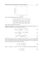
5. Numerical simulation results

This scheme was verified by simulations on a 3-DOF
robot
manipulator
using
MATLAB/SIMULINK.
SOLIDWORKS and SIMMECHANICS of MATLAB/
SIMULINK are used to design the robot's mechanical
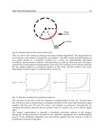
model. An illustration of the robot's kinematics is depicted
in Figure 1. For more details on the structure and
parameters of the robot system, readers can find them in
the study [12]. To demonstrate the proposed strategy's
effectiveness, a comparison is conducted between it and
the conventional SMC [3] in some respects such as
robustness resistance to uncertain components, steadystate errors, and chattering removal capabilities.

4. Proposed controller design
Define respectively 𝑒 = 𝑥1 − 𝑥𝑑 and 𝑒̇ = 𝑥2 − 𝑥̇ 𝑑 as
the position error and velocity error where 𝑥𝑑 and 𝑥̇ 𝑑 stand
for the preferred position and velocity, 𝑥1 and 𝑥2 represent
the measured position and velocity.
Based on the tracking errors, the sliding surface is
designed as:
𝑠 = 𝑒̇ + 𝛽𝑒

(7)

where 𝛽 is positive constant.
Using dynamic (3) to calculate the derivative of Eq. (7)
according to time, we gain:

Figure 1. An illustration of the robot's kinematics

𝑠̇ = 𝑒̈ + 𝛽𝑒̇
= Θ(𝑥, 𝑡) + 𝛿(𝑥, 𝜏𝑑 ) + 𝐽(𝑥1 )𝜏(𝑡) − 𝑥̈ 𝑑 + 𝛽(𝑥2 − 𝑥̇ 𝑑 )
(8)

The robot's task is to follow a following configured
trajectory.
X-axis:
X=0.85-0.01t (m);
Y-axis:
Y=0.2+0. 2 sin( 0.5t) (m);
and
Z-axis:
Z=0.7+0. 2 cos( 0.5t) (m).

Following is a description of how the control law is
designed:
Θ(𝑥, 𝑡) − 𝑥̈ 𝑑   + 𝛽(𝑥2 − 𝑥̇ 𝑑 ) + 𝛿̂
𝜏(𝑡) = −𝐽−1 (𝑥1 ) (
)
+Γ𝑠 + (𝛿̄ + 𝜚)sign(𝑠)

To simulate the influence of interior uncertainties and
exterior disturbances, these terms are assumed as Δ𝐻(𝜑) =
0.3𝐻(𝜑), Δ𝑉(𝜑, 𝜑̇ ) = 0.3𝑉(𝜑, 𝜑̇ ), Δ𝐺(𝜑) = 0.3𝐺(𝜑),

(9)

6 sin(2𝑡) + 4 sin(𝑡/2) + 2 sin(𝑡) + 3[𝜑1 ]0.8

𝜏𝑑 = [5 sin(2𝑡) + 1 sin(𝑡/2) + 2 sin(𝑡) + 2[𝜑2 ]0.8 ] (N. m),
7 sin(2𝑡) + 3 sin(𝑡/3) + 2 sin(𝑡) + 3[𝜑3 ]0.8


8

Nguyen Ngoc Hoai An, Truong Thanh Nguyen, Vo Anh Tuan

]0

0.01[𝜑̇ 1 + 2𝜑̇ 1
and 𝑓𝑟 (𝜑̇ ) = [0.01[𝜑̇ 2 ]0 + 2𝜑̇ 2 ] (N. m).
0.01[𝜑̇ 3 ]0 + 2𝜑̇ 3
The SMC's control input is set as:
Θ(𝑥, 𝑡) − 𝑥̈ 𝑑 + 𝛽(𝑥2 − 𝑥̇ 𝑑 )
𝜏(𝑡) = −𝐽−1 (𝑥1 ) (
)
+Γ𝑠 + (𝛿̄ + 𝜚)sign(𝑠)

(12)

where 𝛽, 𝜚, 𝛿̄ are positive constants and Γ is a positive
diagonal matrix.
The correspondingly selected control parameters for
each controller are reported in Table 1.
Table 1. Selected parameters of the control methods
SMC(12)

1

Parameter
𝛽; 𝜚; 𝛿̄ ; Γ

Proposed
Scheme(9)

𝛽; 𝜚; Γ
𝜋1 ; 𝜋2 ; 𝛼

Value
10; 0.1; 16; diag(10,10,10)
10; 0.1; diag(10,10,10)
10; 60; 2√30

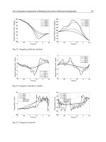
Figure 4. Trajectory tracking errors corresponding
to the X, Y, and Z axis

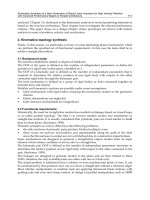
Figure 2. The USOSMO’s outputs

In Figure 2, USOSMO obtains exact estimations of
uncertain terms to offer for the control loop. Accordingly,
the proposed controller uses only the sliding gain 𝜚 to
compensate for the approximation error from the observer
output that contributed to reducing chattering phenomena
in control signals.

Figure 5. Trajectory tracking errors corresponding to each joint

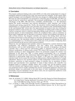
Figure 3. Trajectory tracking performance

The simulation control performance is shown in
Figures 3 – 5. Through a comparison of the tracking
performance in Figures 3 - 5, the proposed controller
achieved better tracking accuracy with small steady-state
control errors and they are much smaller than the SMC’s
control errors because the proposed controller with the
USOSMO has robust properties against uncertain terms.
In addition, the proposed controller’s torques are
smoother than the SMC’s torques, as illustrated in Figure
6. We can see that the chattering behavior in the control


ISSN 1859-1531 - TẠP CHÍ KHOA HỌC VÀ CƠNG NGHỆ - ĐẠI HỌC ĐÀ NẴNG, VOL. 20, NO. 11.2, 2022

input of the proposed controller is mostly eliminated
without losing its robustness.

Figure 6. Control torques: the SMC versus the proposed method

6. Conclusion
The letter developed a SMC scheme based on the
estimated uncertainties using an USOSMO. The
chattering has been effectively reduced and control
performances has been enhanced expressively compared
to conventional SMC because uncertainty estimations
have been achieved with great accuracy and fast
convergence. The effects of input disturbances and
parametric uncertainties can be minimized by a design
with a wide operating range. It was confirmed that the
proposed controller performed well and was efficient. It

is possible to implement the proposed strategy in any
robot manipulator.

9

REFERENCES
[1] T. D. Le, H.-J. Kang, Y.-S. Suh, and Y.-S. Ro, “An online self-gain
tuning method using neural networks for nonlinear PD computed
torque controller of a 2-dof parallel manipulator”, Neurocomputing,
vol. 116, 2013, pp. 53–61.
[2] A. Codourey, “Dynamic modeling of parallel robots for computedtorque control implementation”, Int. J. Rob. Res., vol. 17, no. 12,
1998, pp. 1325–1336.
[3] S. V Drakunov and V. I. Utkin, “Sliding mode control in dynamic
systems”, Int. J. Control, vol. 55, no. 4, 1992, pp. 1029–1037.
[4] H. Wang, “Adaptive control of robot manipulators with uncertain
kinematics and dynamics”, IEEE Trans. Automat. Contr., vol. 62,
no. 2, 2016, pp. 948–954.
[5] S. M. Prabhu and D. P. Garg, “Artificial neural network based robot
control: An overview”, J. Intell. Robot. Syst., vol. 15, no. 4, 1996,
pp. 333–365.
[6] S. K. Spurgeon, “Sliding mode observers: a survey”, Int. J. Syst. Sci.,
vol. 39, no. 8, 2008, pp. 751–764.
[7] N. Boizot, E. Busvelle, and J.-P. Gauthier, “An adaptive high-gain
observer for nonlinear systems”, Automatica, vol. 46, no. 9, 2010,
pp. 1483–1488.
[8] J. Davila, L. Fridman, and A. Levant, “Second-order sliding-mode
observer for mechanical systems”, IEEE Trans. Automat. Contr.,
vol. 50, no. 11, 2005, pp. 1785–1789.
[9] H. K. Khalil, “Extended high-gain observers as disturbance
estimators”, SICE J. Control. Meas. Syst. Integr., vol. 10, no. 3,

2017, pp. 125–134.
[10] A. T. Vo, T. N. Truong, H. J. Kang, and M. Van, “A Robust ObserverBased Control Strategy for n-DOF Uncertain Robot Manipulators with
Fixed-Time Stability”, Sensors 2021, Vol. 21, Page 7084, vol. 21, no.
21, Oct. 2021, p. 7084, doi: 10.3390/S21217084.
[11] E. Cruz-Zavala, J. A. Moreno, and L. M. Fridman, “Uniform robust
exact differentiator”, IEEE Trans. Automat. Contr., vol. 56, no. 11,
2011, pp. 2727–2733.
[12] A. T. Vo, T. N. Truong, and H.-J. Kang, “A Novel PrescribedPerformance-Tracking Control System with Finite-Time
Convergence Stability for Uncertain Robotic Manipulators”,
Sensors 2022, Vol. 22, Page 2615, vol. 22, no. 7, Mar. 2022, p. 2615,
doi: 10.3390/S22072615.