Development of a new method to determine the axial void velocity profile in BWRs from measurements of the in-core neutron noise
Bạn đang xem bản rút gọn của tài liệu. Xem và tải ngay bản đầy đủ của tài liệu tại đây (3.5 MB, 11 trang )
Progress in Nuclear Energy 138 (2021) 103805
Contents lists available at ScienceDirect
Progress in Nuclear Energy
journal homepage: www.elsevier.com/locate/pnucene
Development of a new method to determine the axial void velocity profile in
BWRs from measurements of the in-core neutron noise
Imre Pázsit a , Luis Alejandro Torres b , Mathieu Hursin c,d ,∗, Henrik Nylén e , Victor Dykin a ,
Cristina Montalvo b
a
Division of Subatomic, High Energy and Plasma Physics Chalmers University of Technology, SE–412 96 Gưteborg, Sweden
Universidad Politécnica de Madrid, Energy and Fuels Department, Ríos Rosas 21, 28003, Madrid, Spain
c Paul Scherrer Institut, Nukleare Energie und Sicherheit, PSI Villigen 5232, Switzerland
d Ecole Polytechnique Fédérale de Lausanne (EPFL), Switzerland
e
Ringhals AB, SE-432 85, Väröbacka, Sweden
b
ARTICLE
INFO
Keywords:
Void velocity profile
Void fraction
BWR
Neutron noise
Transit time
Local component
Break frequency method
ABSTRACT
Determination of the local void fraction in BWRs from in-core neutron noise measurements requires the
knowledge of the axial velocity of the void. The purpose of this paper is to revisit the problem of determining
the axial void velocity profile from the transit times of the void between axially placed detectors, determined
from in-core neutron noise measurements. In order to determine a realistic velocity profile which shows an
inflection point and hence has to be at least a third order polynomial, one needs four transit times and hence
five in-core detectors at various axial elevations, whereas the standard instrumentation usually consists only
of four in-core detectors. Attempts to determine a fourth transit time by adding a TIP detector to the existing
four LPRMs and cross-correlate it with any of the LPRMs have been unsuccessful so far. In this paper we thus
propose another approach, where the TIP detector is only used for the determination of the axial position of
the onset of boiling. By this approach it is sufficient to use only three transit times. Moreover, with another
parametrisation of the velocity profile, it is possible to reconstruct the velocity profile even without knowing
the onset point of boiling, in which case the TIP is not needed, although at the expense of a less flexible
modelling of the velocity profile. In the paper the principles are presented, and the strategy is demonstrated
by concrete examples, with a comparison of the performance of the two different ways of modelling the velocity
profile. The method is tested also on velocity profiles supplied by system codes, as well as on transit times
from neutron noise measurements.
1. Introduction
Ever since early work in the mid-70’s on the in-core neutron noise in
BWRs revealed that direct information on the local two-phase flow fluctuations can be obtained through the local component of the neutron
noise (Wach and Kosály, 1974; Behringer et al., 1979), it was thought
that such measurements could also be used to determine the (axially)
local void fraction in the core. Such attempts were also made quite
early by putting forward suggestions on how to extract the local void
fraction from in-core neutron noise measurements (Kosály et al., 1975;
Kosály, 1980). However, as described also recently in Hursin et al.
(2020), the suggested methods were either incomplete and required
either calibration, or several auxiliary conditions, whose fulfilment
was unclear and rather uncertain, or both. Hence, to date no routine
method exists for extracting the local void fraction in BWRs from
measurements.
In the past few years, the interest in determining the local void
fraction by in-core neutron measurements has revived again, not the
least in Sweden (Loberg et al., 2010). As part of this revival, development of such a method was taken up in a joint research project
between Chalmers University of Technology and the Ringhals power
plant, in collaboration with PSI/EPFL. Unlike in the method suggested
by Loberg et al. (2010), in which the void fraction is extracted from
the neutron energy spectrum (which cannot be measured by standard instrumentation), our suggestion was to utilise the information
content in the measured neutron noise by the four axially displaced
LPRM detectors in the same detector string, which constitute the standard instrumentation. The common denominator in the neutron energy
spectrum-based and the neutron noise based methods is that both are
based purely on neutron measurements, and possibly neutron physics
∗ Corresponding author at: Paul Scherrer Institut, Nukleare Energie und Sicherheit, PSI Villigen 5232, Switzerland.
E-mail address: (M. Hursin).
/>Received 23 September 2020; Received in revised form 7 May 2021; Accepted 31 May 2021
Available online 12 June 2021
0149-1970/© 2021 The Authors. Published by Elsevier Ltd. This is an open access article under the CC BY license ( />
Progress in Nuclear Energy 138 (2021) 103805
I. Pázsit et al.
calculations which do not require detailed knowledge of the two-phase
flow structure.
As known from previous work, by using the signals of two detectors
in the same string, one can determine the transit time of the twophase flow between the two detectors. The transit time can be obtained
either from the maximum of the cross-correlation function (CCF) of
the two signals, or from the slope of the phase of the cross-power
spectral density (CPSD), as a function of the frequency (Pázsit and
Demazière, 2010; Hursin et al., 2020). One further possibility is to use
the frequencies where the phase is equal to zero or ±𝜋 (Pázsit and
Glöckler, 1994; Pázsit and Demazière, 2010; Yamamoto and Sakamoto,
2021), or the impulse response function (Czibók et al., 2003; Hursin
et al., 2020). It is generally assumed that since the neutron noise is
induced by the void fluctuations, the transit time is related to the steam
velocity (this point will be returned to below). Hence, in principle,
there is a possibility to determine the void velocity at the detector
positions from the transit times.
However, this in itself is not sufficient to determine the void fraction. To make progress, in a series of works we investigated how
the knowledge of the void velocity at the detector positions could
be utilised to determine the void fraction (Pázsit et al., 2011; Dykin
and Pázsit, 2013; Dykin et al., 2014). One possibility was to use a
relationship between the void fraction and the void velocity through
mass conservation and a known slip ratio. This method has the disadvantage that is not based on purely neutronic measurements, rather it
assumes knowledge of the flow properties. The other possibility was
based on the fact that the neutron noise is induced by the passage of
the fluctuating two-phase flow structure through the so-called detector
field of view, determined by the range of the local component of the
neutron noise (Wach and Kosály, 1974; Dykin and Pázsit, 2013). This
range is determined by an exponent 𝜆(𝑧), which is a spatial decay
constant (with dimensions of inverse length), describing the spatial
decay of the local component. It is a function of the void fraction
(hence also of the axial elevation 𝑧), but independent from all other
thermal hydraulic parameters such as the flow regime or the slip ratio.
For any given void fraction, it can be calculated by reactor physics
methods. Due to the existence of the local component, the auto power
spectral density (APSD) of the neutron detectors will then have a break
frequency at
𝑓 = 𝑣(𝑧) 𝜆(𝑧)
Fig. 1. APSDs of simulated in-core detector signals induced by a bubbly flow at various
elevations (Pázsit et al., 2011).
2014; Yamamoto and Sakamoto, 2016; Yamamoto, 2018; Yamamoto
and Sakamoto, 2021). What regards the flow simulation, even in these
works a bubbly flow was simulated. However, the local component of
the neutron noise, or rather the full neutronic transfer function, was calculated with a frequency dependent Monte-Carlo method with complex
weights. Therefore, the range of the local component is fully realistic
in these calculations, and can be used in practical applications, such
as the evaluation of pilot experiments in research reactors (Yamamoto
and Sakamoto, 2021).
A note on the usage of the word ‘‘void velocity’’ is in order here.
In the neutron noise community it is tacitly assumed that the transit
time deduced from the neutron noise measurements corresponds to
the transit time of the void (steam). However, the neutron noise is
induced by the temporal fluctuations of the reactor material around
its mean value. In a binary or dichotomic medium (fluid-void), it is
represented by the fluctuations of the minority component. At low void
fraction, such as a sparse bubbly flow, the neutron noise is indeed
generated by the fluctuations represented by the void, and hence the
transit time obtained by the noise measurement corresponds to the
transit time of the void. At high void fractions, the fluid becomes
the minority component, hence the neutron noise is generated by the
water droplets/mist, and/or the propagating surface waves of the water
in an annular flow regime. Therefore, in the upper part of the core,
i.e. between the uppermost two detectors, it is more correct to talk
about the transit time of the perturbation.
It is a great advantage of the break frequency method that the break
frequency depends on the transit time of the perturbation through the
detector field of view. Hence, it is completely independent of whether
the fluctuations of the void or the fluid generate the detected neutron
noise. This means that the range 𝜆 of the local component will be
determined correctly, and hence also the break frequency method will
supply the void fraction correctly, since this latter is extracted from
the dependence of 𝜆 on the void fraction. Because of this fact, and
because full realistic calculations of the detector field of view are
underway (Yamamoto, 2018), the break frequency method appears to
be more suitable and effective for determining the void fraction in
operating BWRs.
The above also means that it would be more correct to refer to ‘‘perturbation velocity’’ rather than ‘‘void velocity’’ in this paper. However,
this would be cumbersome and even confusing, and for practical reasons, we will use the terminology ‘‘void velocity’’ or ‘‘steam velocity’’
throughout, on the understanding that in the upper part of the core, it
actually means the velocity of the perturbation, which may differ from
that of the void (steam).
(1)
An illustration of the break frequency between 10 and 15 Hz is shown
in Fig. 1
Since the break frequency can be obtained in a straightforward
way from the detector signal, then, if also the void velocity can be
extracted from the neutron noise measurements, the range 𝜆(𝑧) of the
local component can also be obtained and, from the calculated correlation between the void fraction and 𝜆, the void fraction can also be
extracted. Although this method is not purely based on measurements,
nevertheless similarly to the neutron energy spectrum method, it has
the advantage that it does not require any knowledge on the thermal
hydraulic conditions in the core.
A pilot study on the feasibility of both methods (mass conservation
and break frequency methods) was investigated in simplified models.
A bubbly flow was generated through a Monte-Carlo simulation, with
the help of which the performance of the two methods could be investigated in model cases (Pázsit et al., 2011; Dykin and Pázsit, 2013).
Regarding the first method, a slip ratio equal to unity was assumed.
This is not valid in realistic cases, it was just used for test purposes.
Regarding the break frequency method, the dependence of the range
of the local component on the void fraction was calculated in a simple
analytical model.
Similar numerical studies were performed also by other groups with
the purpose of investigating the possibilities of determining the transit
time from in-core neutron noise measurements, as well as to calculate
the local component of the neutron noise in realistic cases (Yamamoto,
2
Progress in Nuclear Energy 138 (2021) 103805
I. Pázsit et al.
‘‘true’’ profiles as a starting point. From the true profiles, the three
transit times between the four detectors can be calculated, and then
the inversion procedure applied and its accuracy investigated. Since
we do not have access to measurement data with four transit times
or three transit times plus the knowledge of the axial onset point of
the boiling, we need to make some assumptions when investigating
the applicability of the polynomial form. The sensitivity of the results
on the accuracy of these assumptions will be illustrated in model
calculations. We will also investigate the flexibility of the two forms
of the velocity profiles to reconstruct various types of axial velocity
dependences, and the sensitivity of the reconstruction on the correct
assumption on the form of the profile (i.e. starting with a trigonometric
as ‘‘true’’ and performing the reconstruction with the polynomial form,
and vice versa), as well as taking a true polynomial profile with a
given onset point of the boiling and making the reconstruction with a
different onset point as an incorrect guess. A test will be also made with
transit times corresponding to void velocity calculations with a thermal
hydraulic system code. Finally, an attempt will be made to reconstruct
the (unknown) velocities at the detector positions from a measurement
at Ringhals-1, both with the trigonometric and the polynomial velocity
forms. The focus of the investigation is to see which method can
reconstruct the known transit times better, and which inversion method
is more robust and convergent.
Whichever method is used for recovering the void fraction, the
void/perturbation velocity is needed at the detector positions. Elaboration of a method of how the void velocity can be extracted from
the detector signals is the sole objective of this paper. Namely, in incore noise measurements only the transit times of the void between
two axially displaced neutron detectors can be obtained. The transit
times are integrals of the inverse of the velocity, which is not constant
between the detectors. The relationship between the void velocity at
the detector positions, and the transit time between the detector pairs,
is hence rather involved.
Determination of the void velocity at the detector positions is
therefore only possible if a functional form is assumed for the velocity
profile, which depends only on a few parameters, which then can
be determined from the available transit time data. Since the axial
dependence of the velocity has an inflection point, it has to be described
by a non-linear function. The simplest such function, which was also
suggested by Pázsit et al. (2011) and Dykin and Pázsit (2013), and
which is the only one tested so far, is a third order polynomial.
However, a third order polynomial has four parameters. To determine these, one would need four independent transit times, hence
access to five detectors. The standard instrumentation of BWRs comprises only 4 detectors axially at one radial core position, thus one has
access only to three transit times between the three detector pairs.
To solve this problem, it was suggested that one could use, in
addition to the four standard LPRMs (Local Power Range Monitors),
an additional TIP detector (Transverse In-core Probe), by placing the
TIP at an axial position either between the four LPRMs, or outside
these, i.e. in a position different from those of the LPRM positions,
and determine the transit time between the TIP and the nearest LPRM.
This approach was tried in measurements, performed in the Swedish
Ringhals-1 BWR (Dykin et al., 2014). Unfortunately, as is also described
in Dykin et al. (2014), the attempt was unsuccessful. Due to the fact
that, for obvious reasons, the data acquisition for the LPRMs and the
TIP detectors belong to completely separate measurement chains, the
data acquisition is made separately, which made synchronising the
two data acquisitions with a sufficient accuracy impossible. Hence the
transit time between the TIP and any of the LPRMs was not reliable.
The conclusion in Dykin et al. (2014) was that the application of the
TIP detector for acquiring a fourth transit time is not feasible.
Therefore, here we suggest a different strategy. First, we realise that
there is no need for a fourth transit time to determine four parameters
of the velocity profile, either a polynomial or some other form, if
both the axial point of the onset of the boiling, as well as the steam
velocity in this point are known. The onset point of the boiling can
be determined with a TIP detector alone, from the amplitude of its
root mean square noise (RMS) or its APDS, or, alternatively, from
the coherence between the TIP and the lowermost LPRM, if these are
determined as a function of the axial position of the TIP. Neither of
these requires a perfect, or any, synchronisation between the two data
acquisition system. At the onset of the boiling the void velocity can be
assumed to be equal to the inlet coolant velocity, which is known. Thus,
knowledge of these two quantities reduces the number of unknowns of
the axial velocity profile to be determined from four to three.
Second, there exist non-linear functions with an inflection point,
which represent an even higher order non-linearity than a third order
polynomial, but which nevertheless can be parametrised with only
three parameters instead of four. Examples are certain trigonometric
or sigmoid functions. For simplicity these profile types will be referred
to as ‘trigonometric’’. In this case not even the onset point of the boiling
needs to be known; determination of the void profile is then possible
based on solely of the three measured transit times with the standard
instrumentation, without the need for using a TIP detector at all.
In the following, the principles, as well as the applicability of
both types of velocity profile forms (trigonometric and polynomial)
will be investigated in conceptual studies. Various types of velocity
profiles, both trigonometric and polynomial, will be assumed as the
2. The velocity profile and its modelling
2.1. Characteristics of the velocity profile
As is general in reactor noise diagnostics problems, when only a
limited number of measurements is available, obtained from detectors
in a few specified spatial positions, this is not sufficient to reconstruct
the full spatial dependence of the noise source. Inevitably, one needs
to make an assumption on the space dependence of the noise source
in an analytical form, which contains only a limited number of free
parameters. These can then be determined from the limited number of
measurements (Pázsit and Demazière, 2010).
This strategy is easy to follow for localised perturbations, such as
a local channel instability or the vibrations of a control rod, since the
perturbation can be simplified to a spatial Dirac-delta function, either
with a variable strength, or with a variable position. All these cases can
be described by a few parameters, whose physical meaning is obvious,
and the guess on the analytical form is rather straightforward.
What regards the reconstruction of the velocity profile, the case
is more complicated. Here a whole profile (the axial dependence of
the velocity) needs to be reconstructed, and it is not obvious how to
parametrise it. One main difficulty is that, for obvious reasons, no
directly measured velocity profiles are available, which would give
a definite hint on a functional form with only a few parameters to
be determined. Only qualitative information is known either from
calculations with system codes, from common sense considerations, or
from simulations.
An inventory of the available knowledge yields the following. What
regards results from calculations with system codes, there are some
data available from calculations with the system codes TRACE (USNRC,
2008a,b,c) and RAMONA (Wulff, 1984; RAMONA, 2001). Fig. 2 shows
a few profiles from calculations with TRACE, where account was taken
for the fact that the boiling does not start at the inlet, rather at a higher
elevation (Hursin et al., 2017). In Fig. 3, calculations with RAMONA of
the steam velocity in Ringhals 1 in a few selected channels are shown.
RAMONA5 is capable of treating a non-homogeneous two-phase flow,
and the vapour velocity 𝑣𝑔 is related to the liquid velocity 𝑣𝑙 through
the expression
𝑣𝑔 = 𝑆 ⋅ 𝑣𝑙 + 𝑣0
where 𝑆 is the slip factor, and 𝑣0 is the bubble rise velocity (the
vapour velocity relative to stagnant liquid) using the notations in the
3
Progress in Nuclear Energy 138 (2021) 103805
I. Pázsit et al.
get a hint on the possible axial velocity profiles to be investigated. On
the other hand, regarding the void velocity profiles, based on the ever
improving reliability and accuracy of the system codes, one may rely
on the type of the velocity profiles which these codes predict. In this
respect one can draw the conclusion that all the profiles shown above
can be satisfactorily approximated by a 3rd order polynomial. Trying
to fit data from real measurements to such profiles will reveal which
out of the above two types, close to linear increase in the upper part of
the core or a strong inflection point is more likely. A fit to the profiles
obtained from RAMONA calculations will be made in Section 6. A fit
to real measurements will be made in Section 7.
2.2. Possible analytical forms
In our previous works (Pázsit et al., 2011; Dykin and Pázsit, 2013;
Dykin et al., 2014) a third order polynomial was assumed for the axial
dependence of the void velocity:
𝑣(𝑧) = 𝑎 + 𝑏 𝑧 + 𝑐 𝑧2 + 𝑑 𝑧3
(2)
This form has found to have some disadvantageous properties: partly
that the integral of 𝑣−1 (𝑧) w.r.t. 𝑧 does not exist in an analytical form,
and partly that it assumes that the boiling starts at the inlet, i.e. at 𝑧 = 0,
which is not true in practical cases.
The first of these disadvantages does not represent a significant
difficulty, since the unknown parameters 𝑎–𝑑 can also be determined
by numerical unfolding methods, as it will be shown below. Even for
the trigonometrical profile, where the same integral exists in analytical
form, the numerical unfolding method is more effective than root
finding of a highly not-transcendental analytical function in several
variables.
The second property poses somewhat larger problems. Accounting
for the fact that the onset of the boiling is at 𝑧 = ℎ where ℎ is an
unknown, would increase the number of parameters to be determined
to 5. However, as suggested in this work, if the onset point 𝑧 = ℎ of the
boiling is known from measurements, then the third order polynomial
form of (2) can be written in the form
[
]
𝑣(𝑧) = 𝛥(𝑧 − ℎ) 𝑣0 + 𝑏 (𝑧 − ℎ) + 𝑐 (𝑧 − ℎ)2 + 𝑑 (𝑧 − ℎ)3
(3)
Fig. 2. Void velocity profiles simulated by TRACE.
Fig. 3. Void velocity profiles simulated by RAMONA in four neighbouring channels.
where 𝛥(𝑧) is the unit step function, and 𝑣0 is the (known) inlet
coolant velocity. This form contains only three unknowns, which can
be determined from the three measured transit times. This procedure
is suggested for future use, such that the onset point of boiling is
determined by measurements with movable TIP detectors.
Since such measurements are not available at this point, the test
of the polynomial form will be performed by making a qualified guess
on the onset point. The uncertainty of the unfolding procedure with
a polynomial profile can be assessed with respect to the error in the
estimation of the position of the onset point of boiling, which will be
performed in Section 5.2.2.
In addition we propose also to investigate another path. The essence
is the recognition that there exist non-linear functions other than a
third-order polynomial which have an inflection point, and which contain only three free adjustable parameters. These include trigonometric
functions, such as 𝑎 ⋅ atan (𝑏 (𝑧 − 𝑐)), where 𝑎, 𝑏 and 𝑐 are constants, or
the so-called ‘‘sigmoid’’ function, used in the training of artificial neural
networks (ANNs). In the continuation we will refer to such profiles as
‘‘trigonometric’’. For such profiles the onset point of the boiling does
not need to be known. In the next section such a model is proposed,
and a procedure for its use for the unfolding of the velocity profile is
suggested.
Of course, the price one has to pay for the convenience of only
needing to fit three parameters instead of four is that the structure of
the profile is more ‘‘rigid’’ than that of the more general polynomial
form, hence its flexibility of modelling and reconstructing a wide range
of velocity profiles is reduced as compared to the polynomial fitting.
If the onset point of boiling was known, then clearly the polynomial
RAMONA5 user manual (RAMONA, 2001). The slip parameter 𝑆 is
calculated using the option for the Bankoff–Malnes correlation. From
the RAMONA result files, the nodal vapour velocity (also referred to as
steam velocity) of each channel can be extracted.
In Fig. 3, the discontinuity at around 2.5 m is due to the fact that the
fuel assemblies, in which the calculations were made, contain partial
length fuel rods, with a different length in one of the channels. At the
elevation of the end of the partial length, there is an abrupt change in
the void/fuel ratio, hence the sudden change in the void velocity. The
effect of such a discontinuity on the proposed method of the velocity
reconstruction will be assessed in Section 6.
Another possibility is to use results from simulations of a bubbly
flow in a heated channel, which were performed by an in-house Monte
Carlo code. This code was developed earlier and was used in previous
work (Pázsit et al., 2011; Dykin and Pázsit, 2013). Some profiles,
resulting from these simulations, are shown in Fig. 4.
What these figures tell us is that the velocity increases monotonically in the channel from the inlet, first in a quadratic manner,
then the increase slows down, either leading to an inflection point,
or to a linear increase towards the core exit. One has though to keep
in mind that these are all calculated/simulated values, and a direct
measurement of the velocity profiles inside a BWR core will never
be available.Moreover, as was mentioned in the Introduction, in the
upper part of the core, the void velocity can differ from the velocity
of the perturbation (which is just as impossible to measure directly).
Hence, the simulated/calculated velocity profiles are mostly used to
4
Progress in Nuclear Energy 138 (2021) 103805
I. Pázsit et al.
Fig. 4. Void velocity profiles simulated by a Monte-Carlo model of bubbly two-phase flow.
profile would be recommended. It the onset point is not known, it is not
clear whether the use of a trigonometric form, or that of the polynomial
form used with a guess for the axial point of the onset of the boiling
yields better results.
the reflector, represented as an extrapolation length as an independent
parameter, can be accounted for.
With this choice, after integration, the velocity profile is obtained
in the simple form
{
[ (
)]}
𝐻
𝑣(𝑧) = 𝛥(𝑧 − ℎ) 𝑎1 + 𝑐1 sin 𝐵 𝑧 −
(6)
2
3. Construction of a simple non-polynomial velocity profile
with
In order to obtain a velocity profile with an inflection point, which
can be described by only three parameters, we shall assume a very
simple phenomenological model based on simple considerations. The
model does not have any deep physical meaning, or justification. One
of its advantages, besides its simplicity, is that since it is based on a
physical model, whatever coarse it is, it makes it simpler to estimate
the possible range of the model parameters (which is useful in the
inversion process), and in particular it is more straightforward to find
initial guesses of the parameters included to the numerical inversion
procedure than for the polynomial model. Although, the comparative
investigations made later on in this chapter will show that this latter
advantage is not significant in the sense that the polynomial model
is much less sensitive to the correct choice of the starting guess of
the sought parameters than the non-polynomial model.Because of its
simplicity, such a model of assuming the void fraction being proportional to the integral of the heat generation rate was used also in other
works (Yamamoto and Sakamoto, 2016).
Assume that the core boundaries lie between 𝑧 = 0 and 𝑧 = 𝐻 in
the axial direction with a static flux 𝜙(𝑧). Assuming that the boiling
starts at the axial elevation 𝑧 = ℎ, and that there is a simple monotonic
relationship between void fraction and void velocity, and that the latter
at point 𝑧 is proportional to the accumulated heat production between
the boiling onset and the actual position, gives the form
{
}
𝑧
𝑣(𝑧) = 𝛥(𝑧 − ℎ) 𝑣0 + 𝑐
𝜙(𝑧) 𝑑𝑧 .
(4)
∫ℎ
𝑎1 = 𝑣 0 −
and 𝑐1 =
𝑐
𝐵
(7)
A qualitative illustration of a typical velocity profile provided by
this model, referred to as the trigonometric profile, is given below.
To this order, geometrical as well as inlet and outlet velocity data
are taken from the Ringhals-1 plant. The geometrical arrangement is
depicted on Fig. 5, giving the core height and the axial positions of the
detectors from the core bottom. The 4 fixed LPRM positions are marked
on the left, whereas the 7 intermediate positions where TIP detector
measurements were made and tried to be used to generate extra transit
times in Pázsit et al. (2011), are marked on the right. In the present
study only the LPRM positions will be used. The inlet coolant velocity is
𝑣𝑖𝑛 = 𝑣0 = 2 m/s, and the outlet void velocity is about 12 m/s. Assuming
an extrapolation distance of 0.2 m for the flux, and assuming the onset
of the boiling at ℎ = 0.2 m, the static flux and the arising velocity profile
are shown in Fig. 6.
In the next section, the unfolding procedure (the algorithm for the
reconstruction of the velocity profile from the transit times) will be
briefly described. The velocity reconstruction method will then be first
tested on various trigonometric profiles supplied by the above model,
together with those of the polynomial profile (referred to as synthetic
velocity profiles). Thereafter the reconstruction of the velocity profiles
will be tested on the data given by calculations with RAMONA, shown
in Fig. 3. Finally, an attempt will be made to reconstruct the velocity
profile from a Ringhals measurement.
where ℎ and 𝑐 are unknown constants.1 Assume now, for simplicity, a
simple cosine flux shape as
𝜙(𝑧) = cos[𝐵(𝑧 − 𝐻∕2)]
[ (
)]
𝑐
𝐻
sin 𝐵 ℎ −
𝐵
2
4. The unfolding procedure
(5)
In reality, the axial flux shape in a BWR deviates quite appreciably
from a cosine-shaped profile, and moreover that profile is known from
in-core fuel management calculations. Hence, the assumption of the
simple cosine flux profile could be replaced with a more realistic one,
although presumably at the price that the simplicity of the model, and
hence its advantages, would be lost.
In Eq. (5) it is not assumed that 𝐵 = 𝜋∕𝐻, rather 𝐵 is kept as an
independent (unknown) parameter. By allowing 𝐵 < 𝜋∕𝐻, the effect of
First we tried to use the velocity profile given in Eq. (6), since it depends only on three parameters, hence three transit times, derived from
four LPRM signals, should be sufficient for reconstructing the velocity
profile. Eq. (6) has the further property that its inverse is analytically
integrable, thereby giving a possibility to express the transit time 𝑡1,2
of the void between the detector positions 𝑧1 and 𝑧2 , with 𝑧1 < 𝑧2 ,
as analytical functions of the unknown parameters 𝑎1 , 𝑐1 and 𝐵. For
practical reasons we will number the detector positions such that 𝑧1
corresponds to the lowermost detector, LPRM 4, and the transit times
between the detector pairs will be indexed by the position of the lower
detector, i.e. 𝑡1,2 ≡ 𝑡1 etc.
1
As mentioned earlier, if needed, ℎ can be determined by measurements
with a TIP detector.
5
Progress in Nuclear Energy 138 (2021) 103805
I. Pázsit et al.
equation system
𝑡𝑖 (𝑎1 , 𝑐1 , 𝐵) = 𝜏𝑖 ,
(9)
𝑖 = 1, 2, 3
This strategy was tested by choosing detector positions, core size, as
well as inlet coolant velocity and the same value for 𝑐1 which were
used in calculating the profile in the right hand side of Fig. 6. Having
the analytical form of 𝑣(𝑧), the concrete transit times 𝜏𝑖 , 𝑖 = 1, 2, 3 can
be numerically evaluated and used in (9), with the 𝑡𝑖 given in the analytical form (8). For the numerical solution of this non-linear equation
system, the numerical root finding routine NSolve of Mathematica
12.1.1.0 was used (Wolfram Research). However, the root finding did
not converge, even if quite accurate starting values were specified. It
appears that the NSolve routine is primarily designed for treating
polynomial equations, rather than transcendental ones.
Therefore, another path was followed to unfold the parameters of
the void profile from the transit times. Instead of using Nsolve, a kind
of fitting procedure was selected by searching for the minimum of the
penalty function
3
∑
[
𝑡𝑖 (𝑎1 , 𝑐1 , 𝐵) − 𝜏𝑖
]2
(10)
𝑖
as functions of 𝑎1 , 𝑐1 and 𝐵. First the FindMinimum routine of
Mathematica, was used. This procedure worked well and was able to
reproduce the input parameters of the velocity profile. Initially the
analytical form (8) was used for the 𝑡𝑖 (𝑎1 , 𝑐1 , 𝐵). However, it turned out
that defining these latter as numerical integrals with free parameters
𝑎1 , 𝑐1 , 𝐵 worked much faster and with better precision, showing also
that for the unfolding, it is not necessary that the transit times are given
in an analytical form. Consequently, the modified polynomial form of
𝑣(𝑧) in Eq. (3) can also be used, despite that 𝑣−1 (𝑧) is not integrable
analytically.
The unfolding procedure was tested using both the trigonometric
velocity profile given in (6), as well as with the polynomial profile
of Eq. (3). Tests were made with various values of the parameters,
also with combinations that yielded velocity profiles similar to those
in Fig. 2. These extended numerical tests were made by Matlab. The
minimum of the penalty function (10) was found by own MATLAB
scripts. In addition, unlike for the case with Mathematica, for the
trigonometrical profile, using the parameter values obtained from the
minimisation process as starting values to the routine fsolve helped
to successfully solve also the nonlinear system of Eqs. (8), to get the
velocity profile.
Fig. 5. Layout of the measurements.
With these notations, one has
𝑧
𝑖+1
𝑑𝑧
𝑡𝑖 (𝑎1 , 𝑐1 , 𝐵) =
=
∫𝑧𝑖
𝑣(𝑧)
(
)
(
)
⎛
⎛
⎞
⎛
⎞⎞
1
1
⎜ −1 ⎜ 𝑐1 − 𝑎1 tan 4 𝐵(𝐻 − 2𝑧𝑖+1 ) ⎟
⎜ 𝑐1 − 𝑎1 tan 4 𝐵(𝐻 − 2𝑧𝑖 ) ⎟⎟
−1
2 ⎜tan ⎜
√
√
⎟ − tan ⎜
⎟⎟
⎜
⎜
⎟
⎜
⎟⎟
𝑎21 − 𝑐12
𝑎21 − 𝑐12
⎝
⎝
⎠
⎝
⎠⎠
√
𝐵 𝑎21 − 𝑐12
5. Test of the reconstruction algorithm with synthetic profiles
(8)
Our expectation was that in possession of the analytical expressions for
𝑡𝑖 (𝑎1 , 𝑐1 , 𝐵), 𝑖 = 1, 2, 3 in the above form, and having access to given
values of the three measured transit times 𝜏𝑖 , 𝑖 = 1, 2, 3, the unknown
parameters 𝑎1 , 𝑐1 , 𝐵 can be determined as the roots of the non-linear
5.1. Trigonometric profile
Two tests will be shown for illustration, with two different profiles.
We used a more curled and flatter profile, respective, with the following
Fig. 6. Flux and void velocity profile.
6
Progress in Nuclear Energy 138 (2021) 103805
I. Pázsit et al.
Fig. 7. Reconstruction of two trigonometric velocity profiles.
data:
1.
H = 3.68 m;
d = 0.2 m;
h = 0.2 m;
c = 4;
d = 0.8 m;
h = 0.2 m;
c = 3.6;
𝑣0 = 2 m/s.
2.
H = 3.68 m;
𝑣0 = 2 m/s.
The true (=starting) and reconstructed profiles for these two cases
are shown in Fig. 7. The solid red line represents the true profile, and
the broken blue the reconstructed one. It is seen that the inversion
algorithm was able to reconstruct the original profiles in both cases
quite well.
Tests made on a large variety of different profiles revealed that
finding the minimum of the penalty function, Eq. (10), with the Matlab
routine fsolve, the procedure in some cases did not converge to the
true parameters. In some cases the minimum searching ended up by
providing complex numbers for the searched parameters, even if quite
accurate starting values and searching domains were specified. This
lack of convergence is a reason for concern, since in a real application
one does not know the searched parameters and hence cannot specify
good starting values.
However, the fact of sometimes obtaining complex values of 𝑎1 , 𝑐1
and 𝐵 gave the idea of taking only the real part of the search function,
such that the minimisation was performed on the modified penalty
function
3
∑
[
]2
real(𝑡𝑖 (𝑎1 , 𝑐1 , 𝐵)) − 𝜏𝑖
Fig. 8. Reconstruction of several different trigonometric velocity profiles.
Finding correct initial values of the parameters for the minimisation
process was easy, by taking a qualified guess of the void velocity at
the outlet, the velocity gradient at the axial position of the inflection
point of the profile and the void velocity at the position of the second
detector. It seemed that handling the polynomial profile was more
efficient than that of the trigonometric profile. One case of a successful
reconstruction is shown in Fig. 9, where the following data were used:
(11)
𝑖
H = 3.68 m;
With this, the convergence problems experienced previously ceased,
and in all cases the minimisation procedure found the correct parameters for the reconstruction of the initial profile. An illustration of the
performance of the method with a large selection of different profiles
is shown in 8.
h = 0.2 m;
𝑣0 = 2 m/s;
𝑣(𝑧 = 𝐻) = 12.1 m/s.
It is seen in Fig. 9 that the reconstruction is completely successful.
5.2.2. Reconstruction with an unknown boiling onset point ℎ
In this case we assumed a value for the onset point in the reconstruction procedure which was different from the true one. In a practical
case, when no information on the boiling onset point is available,
it is a reasonable choice to assume the position at the boiling onset
halfway between the core inlet and the position of the lowermost
detector, because this minimises the error of the guess. Since the
lowermost detector position is at 0.66 m, we selected ℎ = 0.33 m. Two
reconstructions were made, one by taking ℎ = 0.45 m for the true onset
point, and another by taking ℎ = 0.15 m for the true onset point.
The results of the reconstruction are seen in Fig. 10. It is seen that,
as expected, the reconstruction will not be perfect, especially in the
lower section of the core. However, as it is also seen in the figure, the
only difference between the true and the reconstructed profiles is at
the lowermost part of the core, and the incorrect reconstruction affects
5.2. Polynomial profile
For the tests with the polynomial profile, the form (3) was used. This
form has four fitting parameters. It was tested in two different ways.
First, we assumed that the correct axial position ℎ of the onset of boiling
is known (e.g. from a tip measurement). In that case, there are only the
three parameters 𝑏, 𝑐 and 𝑑 to be fitted. Second, we assumed that the
correct value of ℎ is not known, rather it was guessed incorrectly, with
a certain error. The interesting question was then to see how large an
error this incorrect estimate causes in the reconstruction process.
5.2.1. Reconstruction with a known boiling onset point ℎ
In this case the unfolding worked always correctly and promptly,
without the need of taking the real value of the penalty function.
7
Progress in Nuclear Energy 138 (2021) 103805
I. Pázsit et al.
The overall conclusion of these model tests is that use of the
polynomial profile is preferred to be used in the reconstruction over
the simpler trigonometric profile.
6. Test with velocity profiles obtained from RAMONA
Another test of the unfolding procedure can be made by using the
velocity profiles generated by the RAMONA calculations, shown in
Fig. 3. This is an interesting exercise, even if, as mentioned earlier, the
true void velocity does not agree with the velocity of the perturbation
in the higher upper part of the core, because it uses non-analytical
(non-synthetic) profiles, rather numerically calculated ones. It also
represents a challenge, due to the discontinuity in the velocity profiles,
which arises because of the presence of partial length rods. In such a
case one can count on that the velocity of the perturbation will also
be affected the same way, i.e. it will experience a discontinuity at the
top of the partial-length rod. Hence this exercise will give information
on the possibilities or the reconstruction of the velocity profile for such
cases.
For the test, first the transit times between the detector positions
had to be determined. Since the RAMONA calculations give the velocity
in a number of discrete points (26 positions), for the accurate determination of the transit time, first a piece-wise continuous function was
fitted to the calculated profiles. From the core inlet up to the lower end
of the discontinuity, as well as from the top end of the discontinuity to
the core outlet, a polynomial fit was made. The discontinuity, which
occurs between two adjacent RAMONA points, was represented by a
linear fit. The result of this fitting is shown in Fig. 12.
Thereafter, the transit times were calculated by an integration of
the inverse velocity from the fitted curves, and used in the unfolding
procedure. Due to its larger flexibility, a polynomial fit was used. The
onset point of the boiling, and the steam velocity at this point was
taken from the RAMONA data. The results of the reconstructed profiles
are shown in Fig. 13, and the reconstructed velocities at the detector
positions are listed in Table 1.
Fig. 13 shows that, for trivial reasons, the reconstructed profiles cannot display any discontinuity. However, they reconstruct the RAMONA
velocity profiles quite accurately up to the discontinuity, after which
there is a significant deviation between the true and the reconstructed
values. The reconstructed velocity in this section, i.e. in the uppermost
part of the core, overestimates the true velocity. Accordingly, the steam
velocity values are reproduced quite accurately in the lower three
detectors, whereas there is an error between 5%–10% in the uppermost
detector (Table 1). Regarding this latter detector, one has to add that
it is quite close to the discontinuity, which means an abrupt change in
Fig. 9. Reconstruction of a polynomial velocity profile.
slightly only the velocity at the position of the lowermost detector. The
rest of the profiles, hence also the velocities at the other three detector
positions, are all correct.
5.3. Significance of choosing the right type of profile
One might also be interested to know the significance of choosing
the right type of profile. In other words, to check the performance of the
reconstruction procedure when the true profile is trigonometric, and
the reconstruction is attempted by using a polynomial form, and vice
versa.
The results of such a test are shown in Fig. 11. In the left hand
side figure the true profile is trigonometric, whereas the reconstruction
is made by the assumption of a polynomial form. In the right hand
side figure the opposite case is shown, i.e. when the true profile is
polynomial, whereas the reconstruction is made by the assumption of
a trigonometric form.
It is seen that the use of the polynomial profile is more flexible
than that of the trigonometric profile. It can very well reconstruct a
true trigonometric profile throughout the whole axial range. It has
though to be added, that here it was assumed that the onset point
of the boiling was known. The figure also shows that when the true
profile is polynomial, the trigonometric form has a slight error in the
reconstruction both at low and at high elevations.
Fig. 10. Left figure: trigonometric profile (true) reconstructed by assuming a polynomial profile; right figure: polynomial profile (true) reconstructed by assuming a trigonometric
profile.
8
Progress in Nuclear Energy 138 (2021) 103805
I. Pázsit et al.
Fig. 11. Reconstruction of two polynomial velocity profiles with incorrect values of the boiling onset point ℎ in the reconstruction algorithm. The guessed value is ℎ = 0.33 m
in both cases. Left hand side figure: true value ℎ = 0.45 m; right hand figure: true value is ℎ = 0.15 m.
Table 1
True and reconstructed steam velocities at the detector positions from the RAMONA
calculations. Velocities are in [m/s].
Channel
𝑣1
𝑣2
𝑣3
𝑣4
340
340
341
341
344
344
345
345
3.0130
3.0259
3.1292
3.1751
3.3651
3.4050
3.3249
3.4335
4.3102
4.3000
5.1182
5.1000
6.3977
6.3800
5.9716
5.9500
5.9338
5.9255
7.2838
7.3264
9.2320
9.1922
8.6179
8.5606
6.7269
7.1153
8.3300
8.8727
9.8958
10.8081
9.7551
10.3114
true
reconstructed
true
reconstructed
true
reconstructed
true
reconstructed
In view of the above, it is quite encouraging that despite the discontinuous character of the velocity profile, the true velocity values were
correctly reproduced at 3 of the 4 detectors, and with an overestimation
of the true velocity by only 5%–10% in the uppermost detector. It
can be added that, as is seen in Eq. (1), an overestimation of the
velocity leads to an underestimation of the detector field of view 𝜆.
Due to the inverse relationship between the field of view and the void
fraction, this also means an overestimation of the void content. This
way, one can claim that in cores containing partial length fuel with
characteristic length up to the uppermost detector, the reconstruction
procedure yields a correct value for three lower detectors, and supplies
an upper limit on the void fraction at the position of the uppermost
detector.
Fig. 12. Fitting a piecewise continuous function to the discrete velocity points provided
by RAMONA calculations. Dots: values given by RAMONA. Continuous lines: results of
the fitting.
7. Test with Ringhals-1 data
It might be interesting to test the procedure with pure measurement
data, where the true values of the flow profile parameters are not
known. This has the disadvantage, that in such a case the validity of
the reconstructed velocity profile cannot be verified, but it is a test
of whether the unfolding procedure works when one cannot give a
qualified guess of the starting values for the search of the minimum.
To this end we took real measurement data from Ringhals-1 (Dykin
et al., 2014). In this particular measurement campaign, four identical
measurements were taken, while a TIP detector was placed at the
four LPRM positions, respectively. Since the position of the TIP does
not influence the thermal hydraulic conditions, the four transit times,
obtained from the fitting of the phase curves, can be used for a rough
estimate of the uncertainty of the transit time estimation. The three
transit times for the four measurements, together with the mean values
and the relative standard deviations are given below in Table 2. It is
Fig. 13. Results of the reconstruction of the velocity profiles of RAMONA from the
transit times given by the RAMONA profiles.
the velocities of all phases (fluid and steam). In such a case the concept
of ‘‘local velocity’’ and ‘‘local void fraction’’ becomes problematic, so
reproducing the local void fraction in that position is not a prime
priority.
9
Progress in Nuclear Energy 138 (2021) 103805
I. Pázsit et al.
Table 2
Transit times from Ringhals-1 (from Dykin et al. (2014)). All times are in seconds.
Measurement number
𝜏1
𝜏2
𝜏3
1
2
3
4
0.2712
0.2684
0.2740
0.2765
0.2111
0.2089
0.2114
0.2051
0.1253
0.1272
0.1289
0.1291
Mean
Relative standard deviation
0.2725
0.0128
0.2091
0.0139
0.1276
0.0138
Thus it turned out that the original concern that the case is underdetermined and one may obtain multiple solutions, was not valid
for this case. This is not a proof that this should be the case in all
other measurements, but at least it is reassuring. Significantly more
cases need to be investigated to get a confirmation of the validity of
the procedure, and validation against calculated/simulated values is
desired. Unfortunately, there is no possibility to validate the method
against explicit measurements of void velocity profiles. However, there
is a database of noise measurements available, made in Swedish BWRs
by GSE Power Systems, which at least yield a wide database of transit
time data between four detectors, on which the method can be further
tested (Bergdahl, 2002).
8. Conclusions
The results obtained by both simulations as well as to data from a
system code and from a single application to a real case are promising,
but further work is required in several areas. There is a thorough need
for verification of the method, which in turn requires access to realistic
void velocity profiles. Due to the lack of direct void velocity measurements, the closest possibility for validation is to make measurements
with four LPRMs plus one movable TIP detector to obtain three transit
times and the axial onset position of the boiling, and at the same time
generate high-fidelity realistic void velocity profiles by system codes.
These could be obtained either from dedicated measurements in critical
assemblies or research reactors, or, more likely, from instrumented fuel
assemblies at operating BWRs, such as all three Forsmark reactors, or
Oskarshamn 3. Such validation work is planned in the continuation, as
well as using the validated model for the next step, i.e. to determine
the local void fraction from in-core noise measurements.
Fig. 14. Void velocity profile obtained from Ringhals measurements.
seen that the uncertainty of the transit time estimation is about 1%.
For the velocity reconstruction, the mean value of the transit times was
used.
CRediT authorship contribution statement
Imre Pázsit: Conceptualization, Methodology, Supervision, Writing
- original draft. Luis Alejandro Torres: Methodology, Investigation,
Data curation. Mathieu Hursin: Data curation, Reviewing and editing.
Henrik Nylén: Funding acquisition, Supervision, Data curation. Victor
Dykin: Methodology, Investigation, Data curation. Cristina Montalvo:
Supervision, Data curation, Reviewing and editing.
Since in this case neither the true character of the profile, nor the
values of the corresponding parameters are known, the only assurance
of the successful reconstruction is that the reconstructed values at least
reproduce the transit times properly. One could expect that the task
is underdetermined, i.e. that several void velocity profiles can be constructed which all reproduce the proper transit times, but are otherwise
different, and supply therefore different values for the velocities at the
detector positions.
Declaration of competing interest
The authors declare that they have no known competing financial interests or personal relationships that could have appeared to
influence the work reported in this paper.
Both the trigonometric and the polynomial forms were used in the
attempt of reconstructing the velocity profile. For the initialisation, the
parameters 𝑣0 = 2 m/s and ℎ = 0.3 m were used. It was seen that
the profiles, either trigonometric or polynomial, which were able to
reconstruct the measured transit times, resembled much more to the
TRACE simulations in Fig. 2 without a marked inflection point, rather
than to the more ‘‘curved’’ profiles in Figs. 3–4. The reconstructed
profile, which yielded the best agreement with the measured transit
times, is shown in Fig. 14. There is no calculation of the void velocity
by either TRACE or RAMONA available for this measurement, and
moreover it is not practical either, in view of the difference between
the void velocity and the velocity of the perturbations as mentioned
before. Hence a comparison between the profile reconstructed from the
measurement with curve fitting, to the simulated profile from a system
code, is not practical.
Acknowledgement
The work was financially supported by the Ringhals power plant,
in a collaboration project with Chalmers University of Technology,
Sweden, contract No. 686103-003.
References
Behringer, K., Kosály, G., Pázsit, I., 1979. Linear response of the neutron field
to a propagating perturbation of moderator density (2-group theory of boiling
water-reactor noise). Nucl. Sci. Eng. 72 (3), 304–321.
Bergdahl, B.G., 2002. Brusdata-Bibliotek - Data Från Mätningar och Experiment under
Åren 1985-1995 Konverterade Från Band till CD (Noise Data Library - Data from
Measurements and Experiments during 1985 - 1995, Converted from Tape to CD.
SSM report, GSE Power Systems AB, SKI Rapport 02:6.
Czibók, T., Kiss, G., Kiss, S., Krinizs, K., Végh, J., 2003. Regular neutron noise
diagnostics measurements at the Hungarian Paks NPP. Prog. Nucl. Energy 43 (1–4),
67–74. />Dykin, V., Montalvo Martín, C., Nylén, H., Pázsit, I., 2014. Ringhals Diagnostics and
Monitoring, Final Research Report 2012 - 2014. CTH-NT-304/RR-19, Chalmers
University of Technology, Göteborg, Sweden, URL: />publication/217234/file/217234_Fulltext.pdf.
When comparing the performance of the two methods, i.e. the
trigonometric vs the polynomial profile, it was once again found that
assumption of the polynomial profile in the reconstruction performed
better. This is because it has more free parameters that can be fitted,
and hence this model is more flexible. Finding the proper parameter
values which must be fixed for the search for the minimum of the
penalty function took more trial and error, but also it made possible
to find a better fit in the end.
10
Progress in Nuclear Energy 138 (2021) 103805
I. Pázsit et al.
USNRC, 2008b. TRACE V5.0 Users Guide – Volume 1: Input Specification. Draft Report,
Available on NRC’s online document retrieval system ADAMS since March 2009
with Reference No. ‘‘ML071000103’’.
USNRC, 2008c. TRACE V5.0 Users Guide – Volume 2: Modeling Guidelines. Draft Report, Office of Nuclear Regulatory Research, U.S. Nuclear Regulatory Commission,
Washington, DC, Available on NRC’s online document retrieval system ADAMS
since March 2009 with Reference No. ‘‘ML071720510’’.
Wach, D., Kosály, G., 1974. Investigation of the joint effect of local and global driving
sources in incore-neutron noise measurements. Atomkernenergie 23, 244–250.
Wolfram Research, 2019. Mathematica, Version 12.1.1.0. Wolfram Research, Inc.,
Champaign, IL..
Wulff, W., 1984. A Description and Assessment of RAMONA-3B Mod. 0 Cycle 4:
A Computer Code with Three - Dimensional Neutron Kinetics for BWR System
Transients. NUREG Report, BNL-NUREG 51748.
Yamamoto, T., 2014. Void transit time calculations by neutron noise of propagating
perturbation using complex-valued weight Monte Carlo. In: Proc. PHYSOR 2014
- The Role of Reactor Physics toward a Sustainable Future. The Westin Miyako,
Kyoto, Japan, September 28 - October 3, 2014, (on CD-ROM).
Yamamoto, T., 2018. Implementation of a frequency-domain neutron noise analysis
method in a production-level continuous energy Monte Carlo code: Verification
and application in a BWR. Ann. Nucl. Energy 115, 494–501. />1016/j.anucene.2018.02.008, URL: />pii/S0306454918300628.
Yamamoto, T., Sakamoto, H., 2016. New findings on neutron noise propagation
properties in void containing water using neutron noise transport calculations.
Prog. Nucl. Energy 90, 58–68. />URL: />Yamamoto, T., Sakamoto, H., 2021. Frequency domain Monte Carlo simulations of
void velocity measurements in an actual experimental setup using a neutron
noise technique. J. Nucl. Sci. Technol. 58 (2), 190–200. />00223131.2020.1814176.
Dykin, V., Pázsit, I., 2013. Simulation of in-core neutron noise measurements for
axial void profile reconstruction in boiling water reactors. Nucl. Technol. 183 (3),
354–366.
Hursin, M., Bogetic, S., Dohkane, A., Canepa, S., Zerkak, O., Ferroukhi, H., Pautz, A.,
2017. Development and validation of a TRACE/PARCS core model of leibstadt
kernkraftwerk cycle 19. Ann. Nucl. Energy 101, 559–575. />1016/j.anucene.2016.11.001, URL: />pii/S0306454916305680.
Hursin, M., Pakari, O., Perret, G., Frajtag, P., Lamirand, V., Pázsit, I., Dykin, V., Por, G.,
Nylén, H., Pautz, A., 2020. Measurement of the gas velocity in a water-air mixture
in CROCUS using neutron noise techniques. Nucl. Technol. 206, 1566–1583. http:
//dx.doi.org/10.1080/00295450.2019.1701906.
Kosály, G., 1980. Noise investigations in boiling-water and pressurized-water reactors.
Prog. Nucl. Energy 5, 145–199.
Kosály, G., Maróti, L., Meskó, L., 1975. A simple space dependent theory of the neutron
noise in a boiling water reactor. Ann. Nucl. Energy 2 (2), 315–321. .
org/10.1016/0306-4549(75)90033-X, URL: />article/pii/030645497590033X.
Loberg, J., Österlund, M., Blomgren, J., Bejmer, K.-H., 2010. Neutron detection–
based void monitoring in boiling water reactors. Nucl. Sci. Eng. 164 (1), 69–79.
/>Pázsit, I., Demazière, C., 2010. In: Cacuci, D.G. (Ed.), Noise Techniques in Nuclear
Systems. In: Handbook of Nuclear Engineering, vol. 3, Springer Science, pp.
1629–1737, chapter 14.
Pázsit, I., Glöckler, O., 1994. BWR instrument tube vibrations - interpretation of
measurements and simulation. Ann. Nucl. Energy 21 (12), 759–786. .
org/10.1016/0306-4549(94)90024-8.
Pázsit, I., Montalvo Martín, C., Dykin, V., Nylén, H., 2011. Final Report on the
Research Project Ringhals Diagnostics and Monitoring, Stage 14. CTH-NT-253/RR16, Chalmers University of Technology, Göteborg, Sweden, URL: https://research.
chalmers.se/publication/173819/file/173819_Fulltext.pdf.
RAMONA, 2001. RAMONA-5, User Manual. Technical Report, Studsvik Scandpower AS.
USNRC, 2008a. TRACE V5.0 Theory Manual, Field Equations, Solution Methods
and Physical Models. Draft Report, Office of Nuclear Regulatory Research, U.S.
Nuclear Regulatory Commission, Washington, DC, Available on NRC’s online
document retrieval system ADAMS since February. 2009 with Reference No.
‘‘ML071000097’’.8.
11