Analysis of the Molten salt fast reactor using reduced-order models
Bạn đang xem bản rút gọn của tài liệu. Xem và tải ngay bản đầy đủ của tài liệu tại đây (4.22 MB, 14 trang )
Progress in Nuclear Energy 140 (2021) 103909
Contents lists available at ScienceDirect
Progress in Nuclear Energy
journal homepage: www.elsevier.com/locate/pnucene
Analysis of the Molten Salt Fast Reactor using reduced-order models
Fahad Alsayyari, Marco Tiberga, Zoltán Perkó ∗, Jan Leen Kloosterman, Danny Lathouwers
Delft University of Technology, Faculty of Applied Sciences, Department of Radiation Science and Technology, Mekelweg 15, Delft, 2629JB, The Netherlands
ARTICLE
INFO
Keywords:
Proper orthogonal decomposition
Data-driven
Adaptive
Molten Salt Fast Reactor
Uncertainty and sensitivity analysis
Transient analysis
ABSTRACT
In this paper, we present a reduced-order modeling approach to study the Molten Salt Fast Reactor (MSFR). Our
approach is nonintrusive and based on the proper orthogonal decomposition method. We include adaptivity
in selecting the sampling points both in time and parameter space. Steady-state and transient analysis were
both performed using the developed models. In the steady-state analysis, we capture the effect of 30 model
parameters on the spatial distributions of fission power and temperature, and on the multiplication factor.
The dimensionality of the fission power was reduced from the 104288 nominal dimensions in the physical
space to 10 dimensions in the reduced space, whereas the temperature was reduced from 220972 dimensions
to 3. The reduced model was then used for uncertainty and sensitivity study of the maximum temperature in
the reactor and the multiplication factor. In the transient analysis, the reduced model captured the effect of
perturbations in the flow rate of salt in the intermediate circuit on the fission power density and temperature.
The reduced models were successfully tested on a set of points that were not part of the snapshots used during
the construction stage.
1. Introduction
Molten salt reactors have gained interest due to their potential
safety, reliability, and sustainability (Generation IV International Forum, 2002). Different designs of this concept have been proposed in
the literature Dolan (2017). In this work, we consider the Molten
Salt Fast Reactor (MSFR) (Allibert et al., 2016). A key design feature
of this unmoderated reactor is the use of a liquid salt fuel, which
also plays the role of the coolant. This design introduces a unique
modeling challenge because of the tightly coupled neutronics and
thermal-hydraulics phenomena (e.g., transport of delayed neutron precursors, distributed thermal energy deposition directly in the coolant,
a strong negative temperature feedback coefficient). To address these
challenges, high-fidelity coupled models are used to provide an insight
into the behavior of the reactor (e.g., Aufiero et al., 2014, Fiorina et al.,
2014, Laureau et al., 2017, Cervi et al., 2019, Tiberga et al., 2020b). For
safety assessment applications, an accurate and explicit quantification
of the propagation of uncertainties through these complex models
is required (International Atomic Energy Agency, 2019). Quantifying
uncertainties and analyzing sensitivities in reactor physics can be accomplished using adjoint methods (Gilli et al., 2013; Perkó et al., 2013).
However, adjoint-based methods require the availability of an adjoint
solver, which might not always be feasible for coupled problems.
Another approach is using forward-based methods, which requires
repeated evaluation of the high-fidelity model for different parameter
configurations (Cacuci, 2003). For example, automatic differentiation
tools can be used to sample the forward model and reconstruct a
discrete version of the adjoint problem (Marta et al., 2007). However,
for large-scale, coupled, high-fidelity models with multiple input parameters such approaches are computationally demanding. For such
applications, reduced-order modeling (ROM) techniques can be used to
simplify the high-fidelity model and produce an efficient, cheap, and
accurate model of the system.
Amongst the classical ROM methods found in literature, proper
orthogonal decomposition (POD) is the method most suited for nonlinear systems (Antoulas et al., 2001; Schilders et al., 2008; Benner
et al., 2015). In the POD approach, a reduced basis space for the
system is built using snapshots of the high-fidelity model. In nuclear
reactor application, POD has been applied to solve criticality eigenvalue
problems (Buchan et al., 2013; Senecal and Ji, 2019; German and
Ragusa, 2019; Prince and Ragusa, 2020), for fuel pin reactor core calculations (Cherezov et al., 2018), in fuel burnup calculations (Castagna
et al., 2020), in thermal hydraulics modeling (Vergari et al., 2020), in
stability analysis (Prill and Class, 2014; Manthey et al., 2019), in spent
fuel pool modeling (Escanciano and Class, 2019), and to model the lead
cooled fast reactor (Sartori et al., 2016). In all of these applications, the
original set of model equations were projected onto the constructed
reduced basis. Projection-based approaches are intrusive because of
the need to access the operator of the original high-fidelity model in
∗ Corresponding author.
E-mail address: (Z. Perkó).
/>Received 13 June 2020; Received in revised form 12 July 2021; Accepted 27 July 2021
Available online 7 August 2021
0149-1970/© 2021 The Author(s). Published by Elsevier Ltd. This is an open access article under the CC BY license ( />
Progress in Nuclear Energy 140 (2021) 103909
F. Alsayyari et al.
the size of the state space (representing, for example, space, angle, and
energy). We consider 𝑓 as a black-box model, which can either describe
single physics or coupled multi-physics code, that is,
order to employ the projection. In cases where the high-fidelity model
is a legacy coupled solver or closed-source, intrusive approaches are
not applicable. Moreover, the stability of the high-fidelity model is not
preserved in the reduced model with the use of projection-based POD
methods (Amsallem and Farhat, 2012).
To overcome these issues, nonintrusive approaches have been proposed in the literature, which are techniques that can be wrapped
around the high-fidelity solver and avoid the need to access the original
set of equations. Nonintrusive spectral projection methods such as
polynomial chaos expansion (PCE) is one approach for uncertainty
quantification applications (Perkó et al., 2014a,b), which has been
applied to a molten salt fueled system (Santanoceto et al., 2021b) and
to perform a preliminary uncertainty and sensitivity analysis of the
MSFR steady-state (Santanoceto et al., 2021a). However, such methods
do not reduce the dimensionality of the high-fidelity model. Dynamic
Mode Decomposition (DMD) is a nonintrusive model order reduction
method that has been employed to model the MSFR (Ronco et al.,
2020). DMD constructs a linear operator from a sequence of snapshots
of the system. Then, a reduced model preserving the dynamics of the
original system is formulated, which can be used for transient analysis
and control applications (Tu et al., 2014). Propagating uncertainties in
the initial conditions has also been studied using DMD (Takeishi et al.,
2017; Abdo et al., 2019). However, for problems with parametrized
models where uncertainty and sensitivity analysis for multiple model
input parameters are to be studied, applying DMD is cumbersome.
An alternative ROM approach is through a nonintrusive POD implementation, where a surrogate model is trained to compute the
POD coefficients instead of projecting the model equation onto the reduced basis. In nuclear reactor applications, a Range Finding Algorithm
(RFA) has been used in Huang et al. (2017) to build the reducedbasis subspace(referred to as active subspace) combined with a simple
polynomial surrogate for the POD coefficients. Hybrid approaches aiming to simultaneously reduce the dimensionality of both the state and
the input variables using RFA have also been explored (Abdel-Khalik
et al., 2013; Bang et al., 2015). We have proposed a nonintrusive
adaptive POD algorithm in Alsayyari et al. (2019). A key difference
in our developed algorithm is the adaptive sampling of the highfidelity model as opposed to random or a priori uniform sampling
employed by the RFA. Our algorithm is based on adaptive sparse grids
technique, which is suited for problems with higher dimensional input
spaces. An uncertainty and sensitivity application of the algorithm on
a simplified two-dimensional molten salt fueled system was presented
in Alsayyari et al. (2020), where we have also addressed handling
systems with multiple-outputs. We have presented an extension of
the algorithm in Alsayyari et al. (2021) to deal with time-dependent
parametrized problems. In this work, we investigate the MSFR reactor
using the developed algorithm, which demonstrates the capability of
the algorithm on a large-scale, three-dimensional MSFR model. We
consider two applications. The first is a steady-state reduced model for
uncertainty and sensitivity analysis of 30 model parameters. The second
is a transient reduced model, which can be used for transient analysis
and control applications.
The remainder of the paper is organized as follows: Section 2
presents an introduction to the problem formulation and the POD
method. A summary of the adaptive sampling algorithm is presented in
Section 3. Then, a description of the MSFR model is given in Section 4.
The results for the steady-state analysis along with the uncertainty
and sensitivity study are given in Section 5. We present the results of
the transient study in Section 6. Finally, conclusions are discussed in
Section 7.
(1)
𝝓 = 𝑓 (𝒑).
The high-fidelity model 𝑓 can be evaluated at any given 𝒑𝑞 and
produce an output 𝝓𝑞 (i.e., 𝝓𝑞 = 𝑓 (𝒑𝑞 )). We are interested in finding an approximation for 𝝓𝑞 without the use of the computationally
intensive 𝑓 . For this task, we build a reduced model that produces an
̃ 𝑞 , which takes the form of
approximation 𝝓
̃𝑞 =
𝝓
𝑟
∑
(2)
𝑐𝑔 (𝒑𝑞 )𝒖𝑔 ,
𝑔=1
where 𝒖𝑔 is the 𝑔th basis vector in the reduced basis space, 𝑐𝑔 (𝒑) is the
corresponding coefficient, which is a function of the parameter 𝒑, and
𝑟 is the size of the reduced basis space. The POD approach constructs
a reduced basis space from snapshots of the state vectors 𝝓 such that
the error is minimized in a least square sense, that is, it solves the
minimization problem
‖
𝑟
∑
‖
min ‖
𝝓−
𝑐𝑔 (𝒑)𝒖𝑔
‖
𝒖𝑔 ‖
𝑔=1
‖
‖
‖
‖ .
‖
‖ 2
‖𝓁
(3)
The basis vectors are defined to be orthonormal (i.e., ⟨𝒖𝑔 , 𝒖ℎ ⟩ = 𝛿𝑔ℎ ,
where ⟨., .⟩ indicates the scalar product). The reduced basis space can
be found using the method of snapshots. Let 𝑀 be a matrix collecting
snapshots of the solution 𝝓 at some selected values of 𝒑, that is,
𝐌 = [𝝓1 , 𝝓2 , … , 𝝓𝑠 ]
∈ R𝑛×𝑠 ,
(4)
where 𝝓𝑞 is the solution of the high-fidelity model (𝑓 ) at parameter
value 𝒑𝑞 , and 𝑠 is the number of selected snapshots. Note that for transient problems where 𝑓 computes a solution 𝝓 that is time-dependent,
we consider the time to be a parameter, rather than an independent
variable — that is, 𝒑 includes time as one of the parameters. Such a
formulation allows for time adaptive sampling as described in Alsayyari
et al. (2021).
The basis vectors are then found to be the left singular vectors of
the singular value decomposition (SVD) applied to the matrix 𝑀, that
is, let 𝑀 be decomposed using SVD as 𝑀 = 𝑈 𝑆𝑉 ⊤ , then 𝒖𝑔 ∀ 1 ≤ 𝑔 ≤ 𝑟
are the first 𝑟 column vectors of 𝑈 . The size of the reduced space is
determined by 𝑟, which can be chosen to truncate 𝑈 such that the
sum of the squared singular values (𝜎) corresponding to the neglected
singular vectors is below a predefined threshold 𝛾tr .
∑𝑛
2
𝑔=𝑟+1 𝜎𝑔
< 𝛾tr .
(5)
∑𝑛
2
𝑔=1 𝜎𝑔
Once the basis vectors are known, we can use the orthogonality of
the space to compute the coefficients at the sampled point (𝒑𝑞 ) as
𝑐𝑔 (𝒑𝑞 ) = ⟨𝒖𝑔 , 𝝓𝑞 ⟩.
(6)
3. Adaptive sampling
Using the values of the coefficient 𝑐𝑔 (𝒑) at the sampled points, one
can train a surrogate model to compute the solution of the system at
any point. Different surrogate models can be employed for such a task.
To deal with higher dimensional input spaces, we choose the Smolyak
sparse grid interpolation technique. The hierarchical structure of the
interpolant allows for the desired adaptive strategy, which can further
reduce the burden of dealing with high dimensional spaces. This section
is devoted to summarize the developed adaptive algorithm, which is
detailed in Alsayyari et al. (2019).
Our implementation of the sparse grid technique uses localized
adaptive sampling. Without loss of generality, the 𝑑-dimensional space
of the input parameter 𝒑 is mapped to a unitary hypercube [0, 1]𝑑 . The
sparse grid technique first generates unidimensional nodes along each
2. Proper orthogonal decomposition
Consider a general high-fidelity model that is described by a function 𝑓 ∶ R𝑑 → R𝑛 , which maps input parameter 𝒑 ∈ R𝑑 to a state (field)
vector 𝝓 ∈ R𝑛 , where 𝑑 is the size of the input space (representing,
for example, material properties, and boundary conditions), and 𝑛 is
2
Progress in Nuclear Energy 140 (2021) 103909
F. Alsayyari et al.
second is to have a descendant point with an error above 𝛾int . Points
that do not meet any of the conditions are added to a set of inactive
points. The error is computed in the 𝓁 2 norm as
‖
̃ 𝑘‖
‖𝝓𝑞 − 𝝓
𝑞‖
‖
‖𝓁2
,
(10)
𝑒𝑘𝑞 =
‖ ‖
‖𝝓𝑞 ‖ 2 + 𝜖
‖ ‖𝓁
where 𝝓𝑞 is the solution returned by the high-fidelity code (𝑓 ) at point
̃ 𝑘 is the approximation produced by the reduced model at the point
𝒑𝑞 , 𝝓
𝑞
𝒑𝑞 and iteration 𝑘, and 𝜖 is an offset introduced for cases when the norm
of the solution is near-zero.
At iteration 𝑘, a surrogate model for the POD coefficient 𝑐𝑔 (𝒑) is
built as
Fig. 1. Illustration of the first 4 levels of the tree structure, where 0.5 is the root of
the tree and nodes are added at half the distances between the previous nodes. Each
node has 2 children except the nodes at level 2 where each has one child only.
dimension. Then, points in the parameter space are formed by a specific
combination of the generated unidimensional nodes. Different choices
for the unidimensional node generation rule are possible. However, we
choose the equidistant rule to increase the separation between points.
The unidimensional nodes are arranged in a tree structure as shown
in Fig. 1. Each level is assigned an index 𝑖 and contains several nodes.
Nodes are added at each level at half the distances between the nodes
from the previous levels. Each node is connected to two children at the
next level (𝑖 + 1) and one father from the previous level (𝑖 − 1). The root
node is considered a father for itself. There is, however, an exception
at level 𝑖 = 2, where each node has one child because these nodes mark
the boundaries of the unit hypercube.
Each node in the tree can be uniquely identified with the level index
𝑖 and an index 𝑗. For each node from the tree 𝑝𝑖𝑗 along dimension 𝑙, we
can build a basis function 𝑎𝑖 𝑖 (𝑝) as
𝐴𝑘,𝑑 (𝑐)(𝒑) = 𝐴𝑘−1,𝑑 (𝑐)(𝒑) + 𝛥𝐴𝑘,𝑑 (𝑐)(𝒑) ,
where 𝐴𝑘,𝑑 (𝑐)(𝒑) is the Smolyak interpolation operator applied to 𝑐(𝒑)
that depends on the iteration 𝑘 and dimension of the input space 𝑑.
For the initialization (𝑘 = 0), we enforce 𝐴0,𝑑 (𝑐)(𝒑) to be zero. The term
𝛥𝐴𝑘,𝑑 (𝑐)(𝒑) is defined as
𝑚𝛥
𝛥𝐴𝑘,𝑑 (𝑐)(𝒑) =
𝛩𝑛 (𝒑) =
ℎ .
𝑖
𝑎 𝑙𝑖𝑙 (𝑝𝑙 ),
(13)
𝑝𝑛,𝑙
𝑤𝑘𝑛 = 𝑐(𝒑𝑛 ) − 𝐴𝑘−1,𝑑 (𝑐)(𝒑𝑛 ).
(14)
At each iteration, a trial set is generated from the forward points of
the important set. The model is tested on each point within the trial
set. To provide an estimate for the global error in the reduced model
at iteration 𝑘 (𝜀𝑘 ), an appropriate norm can be chosen over the error
defined in Eq. (10). In this work, we have chosen the maximum norm
such as the reduced model error is defined by
(7)
𝜀𝑘 = max 𝑒𝑘𝑞
∀1 < 𝑞 < 𝜏 𝑘 ,
(15)
𝜏𝑘
where
is the cardinality of the trial set at iteration 𝑘. However, 𝜀𝑘
only provides an estimate of the error in the reduced model and is not
rigorous.
A point 𝒑 in parameter space is formed by combining nodes from all
𝑖
𝑖
dimensions (i.e., 𝒑 = (𝑝𝑗1 , … 𝑝𝑗𝑑 )). Extending the tree structure to points
1
𝑑
in parameter space allows us to define forward points. The first forward
𝑖
𝑖
points for a point 𝒑 along the first dimension are (𝑏(𝑝𝑗1 ), … 𝑝𝑗𝑑 ), where
1
𝑑
𝑏(𝑝) is a function that returns the children of the node 𝑝. In general,
𝑖𝑙
𝑖
𝑖1
the forward points along the 𝑙th dimension are (𝑝𝑗 , … , 𝑏(𝑝𝑗 ), … 𝑝𝑗𝑑 ).
1
𝑙
𝑑
Because each node has at most two children, each point has at most
2𝑑 forward points. We can also define backward points in the same
manner by applying a function 𝑏∗ (𝑝), which returns the father of the
node. Therefore, each point has at most 𝑑 backward points. Recursively
generating the forward points creates the set of descendant points.
On the other hand, the ancestor points for a point 𝒑 are formed by
recursively generating backward points until the root point (0.5, … , 0.5)
is reached.
The adaptive algorithm is iterative. In every iteration, a subset of
points is selected and marked important from a set of trial points. Let
the iteration number be 𝑘 and a set that collects the selected important
points at each iteration 𝑘 be 𝑘 . The union of the important points sets
(𝑘 ) from all iterations up to 𝑘 forms the set of selected grid points 𝑘 ,
that is,
𝑘
⋃
(12)
The surplus 𝑤𝑘𝑛 is defined as the difference between the interpolated
value and the true value of the coefficient at 𝒑𝑛 ,
where the dependence on the dimension 𝑙 is dropped for notational
convenience. The level parameter 𝑚𝑖 is defined as follows:
{
1
if 𝑖 = 1,
𝑚𝑖 =
(8)
2𝑖−1 + 1 if 𝑖 > 1.
𝑘 =
𝑑
∏
𝑙=1
𝑝
1
< 𝑖
if
,
𝑚 −1
otherwise,
𝑤𝑘𝑛 𝛩𝑛 (𝒑),
where 𝑚𝛥𝑘 is the cardinality of the set 𝑘 . The function 𝛩𝑛 (𝒑) is the
𝑑-variate basis function for the point 𝒑𝑛 ∈ 𝑘 ,
𝑎11 = 1 if 𝑖 = 1,
|𝑝 − 𝑝𝑖𝑗 |
𝑘
∑
𝑛=1
𝑝𝑗
⎧
⎪1 − (𝑚𝑖 − 1) ⋅ |𝑝 − 𝑝𝑖𝑗 |,
𝑎𝑖 𝑖 (𝑝) = ⎨
𝑝𝑗
⎪0,
⎩
(11)
Algorithm
In the initialization step (𝑘 = 0), we select the root point at the
center of the hypercube (0.5, 0.5, … , 0.5) and evaluate the high-fidelity
model 𝑓 . That point is added to the important set 0 , and the snapshot
is added to the matrix 𝑀. Then, set 𝑘 = 1 and do
1. Generate the forward points of the points in 𝑘−1 ;
2. Add points that have all their backward points in 𝑘−1 (defined
as in Eq. (9)) to the trial set;
3. Evaluate the high-fidelity model 𝑓 at the points in the trial set;
4. Compute the coefficients 𝑐𝑔 (𝒑) at the points in the trial set using
𝐴𝑘−1,𝑑 (𝑐)(𝒑);
5. Compute the error at every point in the trial set using Eq. (10);
6. If the maximum found error (𝜀𝑘 ) was below a prescribed global
tolerance 𝜁, terminate; Otherwise, continue;
7. Find the important points 𝑘 ;
8. Add the snapshots corresponding to the important points in 𝑘
to the matrix 𝑀;
9. Perform SVD on the matrix 𝑀 to extract the reduced basis;
10. Use Eqs. (11)–(14) to construct 𝐴𝑘,𝑑 (𝑐)(𝒑);
11. Set 𝑘 ← 𝑘 + 1 and go to Step 1.
(9)
ℎ=0
A point 𝒑𝑞 is marked as important if it satisfies one of two conditions. The first is to have an approximation error 𝑒𝑞 above a defined
threshold 𝛾int with all ancestors of that points included in 𝑘 . The
For a detailed description of the algorithm, see Alsayyari et al. (2019).
3
Progress in Nuclear Energy 140 (2021) 103909
F. Alsayyari et al.
Fig. 3. Computational scheme of the multi-physics tool constituting the high-fidelity
MSFR model. DGFlows is the CFD code, while PHANTOM-S𝙽 is the neutronics code.
Data are exchanged at each iteration between the two solvers to model the coupled
physics phenomena characterizing the MSFR (Tiberga et al., 2020b).
Fig. 2. A schematic illustration of the main design features of the MSFR fuel circuit.
4. MSFR model
This section presents the MSFR main design features and modeling
approach. A more detailed description of the model can be found
in Tiberga et al. (2020b) and the references within.
A schematic illustration of the fuel circuit is shown in Fig. 2. The
reactor core is a toroidal cavity where the liquid fuel salt (a mixture of
lithium, thorium, and fissile nuclides fluorides) can flow freely without
any moderator or control rod. Sixteen identical sectors branch out from
the central cavity. Each sector contains a pump, a heat exchanger, and
a unit for the separation and treatment of the helium gas dispersed
in the fuel salt to control reactivity and remove metallic fission products (Delpech et al., 2009). A blanket with fertile salt surrounds the
cavity while reflectors are placed at the top and bottom of the core.
The heat exchangers transfer thermal energy to the intermediate circuit
filled with inert molten salt, which in turn, delivers the heat to the
energy conversion system consisting of a conventional Joule-Brayton
cycle. Table 1 summarizes the main MSFR design parameters.
The reactor was modeled using an in-house multi-physics tool,
which couples an incompressible Reynolds-averaged Navier–Stokes
solver (DGFlows) (Tiberga et al., 2020a; Hennink et al., 2021) with
an 𝑆𝑁 multi-group neutronics code (PHANTOM-S𝙽 ) (Kópházi and Lathouwers, 2012). The latter is equipped with transport equations for
the delayed neutron precursors to model their movement. Both codes
employ the discontinuous Galerkin finite element method for space
discretization and implicit backward differentiation formulae (BDF)
time schemes. Fig. 3 displays the structure of the multi-physics tool
and the data exchanged between the codes. PHANTOM-S𝙽 receives the
average temperature on each element (𝑇𝑎𝑣𝑔 ) and corrects the cross sections accordingly with respect to a library at the reference temperature
𝑇0 . The corrections take into account the effects of density feedback
(which has a linear dependence on temperature) and Doppler feedback
(which has a logarithmic dependence). The velocity and turbulent
viscosity fields (𝐮 and 𝜈𝑡 ) are also taken from DGFlows as another
input to solve the delayed neutron precursors equation. Then, the
fission power density (𝑃𝑓 𝑖𝑠𝑠 ) is transferred to DGFlows as it constitutes
the right-hand side of the energy equation. The steady-state solution
is sought by iterating the solvers until convergence (four iterations
are typically sufficient). On the other hand, transient simulations are
performed with a loose-coupling strategy, first computing a time-step
with DGFlows and then calling PHANTOM-S𝙽 to solve the neutronics
problem. We refer the reader to Tiberga et al. (2019, 2020b) for a more
comprehensive description of the coupled code.
Because of the symmetry in the reactor design, we modeled only one
recirculation loop. The geometry considered is reported in Fig. 4. While
the neutron flux is calculated in the reflectors and the blanket, the CFD
code (DGFlows) neglects heat transfer in these regions. Fig. 5 shows
Fig. 4. Geometry of the MSFR recirculation loop used for simulations, showing the
main regions considered in the model (Tiberga et al., 2020b).
the meshes used in this study. Neutronics calculations were performed
on an unstructured mesh consisting of 26072 tetrahedra (of which
21489 are in the fuel salt domain). This mesh is finer in the core region,
where neutron importance is high, and coarser in the external sector.
This master mesh was then refined once uniformly in the outer-core
region to obtain the CFD mesh, which consists of 55243 elements. A
second-order polynomial was used for the velocity discretization, while
a first order polynomial was used for all other quantities.
The fuel salt composition is reported in Table 2, along with some
physical properties that were fixed and selected for the uncertainty
analysis study of Section 5. The neutron energy range was condensed
into six groups, with boundaries shown in Table 3. Delayed neutron
precursors were grouped into eight families. All neutronics data were
evaluated at temperature 𝑇0 = 900 × 100 K with Serpent (Leppänen
et al., 2015) using the JEFF-3.1.1 data library (Santamarina et al.,
2009).
For the CFD calculations, symmetry boundary conditions were imposed at the wedge sides, and standard wall-functions with adiabatic
conditions were assumed at all walls. For the neutronics calculations,
reflective boundary conditions were assumed at the sides of the wedge,
while vacuum conditions were imposed elsewhere. For the transport
of the precursors within the fuel salt, homogeneous Neumann and
no-inflow conditions were imposed at all walls.
Lacking detailed design specifications for the primary heat exchanger, salt cooling was modeled via a volumetric heat sink term equal
(
)
to ℎint,0 𝑇int,0 − 𝑇 , where ℎint,0 and 𝑇int,0 are the nominal volumetric
heat transfer coefficient and average temperature of the intermediate
salt whose values are reported in Table 1. The fuel pump was modeled with a momentum source term, and buoyancy was taken into
account through the Boussinesq approximation (the reference density
and thermal expansion coefficient are reported in Table 2). We considered the flow field to be fixed at the nominal state because natural
convection has a negligible contribution to the total nominal flow rate,
and the pump specifications were fixed throughout the analyses in
4
Progress in Nuclear Energy 140 (2021) 103909
F. Alsayyari et al.
Table 1
Main design parameters for MSFR model in the nominal case (Allibert et al., 2016; Gérardin et al., 2017).
Parameter
Value
Total thermal power [MW]
Total fuel salt volume [m3 ]
Fuel salt circulation time [s]
Average fuel salt temperature [K]
Minimum fuel salt temperature [K]
Average intermediate salt temperature [K]
Pressure drop across heat exchanger [bar]
[
]
Volumetric heat transfer coefficient with intermediate salt MW∕m3 K
3000 × 100
18 × 100
4 × 100
973.15 × 100
923.15 × 100
908.15 × 100
4 × 100
19.95 × 100
Fig. 5. Mesh adopted for the MSFR model. The neutronics mesh (left), corresponding to the master-mesh, consists of 26072 tetrahedra (21489 in the fuel salt domain), while the
CFD mesh (right) has 55243 elements. The latter is derived by refining the former once uniformly in the outer-core region.
Table 2
Properties of the fuel salt mixture (Bene˘s et al., 2013).
Property
Value or equation of state
Composition [%mol]
Density [kg∕m3 ]
Dynamic viscosity [Pa s]
Thermal expansion
coefficient [K −1 ]
Melting point [K]
LiF(77.5 × 100 )-ThF4 (6.6 × 100 )-enr UF4 (12.3 × 100 )-(Pu-MA)F3 (3.6 × 100 )
4306.7 × 100
6.187 × 10⁻⁴ exp (772.2∕ (𝑇 (K) − 765.2))
1.9119 × 10⁻⁴
854.15 × 100
this work. Moreover, since we are interested in reactor steady-state
and operational transients, decay heat was not taken into account. For
the transient calculations described in Section 6, the time-dependent
equations were discretized with the second-order BDF scheme with a
fixed time-step size of 0.1 × 100 s.
selected parameters are reported in Table 4. These nominal values are
theoretical as the actual salt properties and the associated uncertainties
are still under investigation. However, for the propose of this work,
we assume an uncertainty following a Gaussian distribution for all
parameters with a mean (𝜇) equal to the nominal value and a standard
deviation (𝜎) taken as 5% of the mean.
5. Steady-state analysis
5.1. Construction of the reduced model
In this section, we study the effect of selected parameters of interest
on three outputs: fission power density (𝑷 fiss ), temperature distribution
(𝑻 ), and the multiplication factor, 𝑘ef f . The fission power density 𝑷 fiss
is computed on the neutronics mesh with 104288 unknowns (nominal
dimensionality) while the temperature 𝑻 is computed on the CFD mesh
with 220972 unknowns. This analysis is performed on the steady-state
model of the MSFR with a fixed reactor power of 3000 MW. However,
since we are modeling 1/16th of the reactor, the observed nominal
power is 187.5 MW. The selected parameters to be investigated were
specific heat capacity of the fuel salt (𝑐𝑝 , influencing the temperature
distribution), heat conductivity of the fuel salt (𝜅), fission cross sections
for the six energy groups (𝛴𝑓 ,𝑔 ), capture cross sections for the six energy
groups (𝛴𝑐,𝑔 ), delayed neutron fractions for eight families of precursors
(𝛽𝑖 ), and corresponding decay constants (𝜆𝑖 ). The nominal values of the
Our implementation of the adaptive approach was developed for
bounded input domains. For this reason, we consider the Gaussian distribution to be truncated. Truncating the Gaussian distribution, in this
case, is a valid approximation because the parameter uncertainties we
are considering are epistemic. Therefore, we are not altering a random
process but rather limiting the scope of analysis to the region with
the highest probability of having the true value. Moreover, truncating
the distribution prevents unphysical values of the parameter, such as
negative 𝛽. The truncation was selected to be at 3𝜎, retaining 99.7%
of the probability range. This implies that the range of variation for all
parameters is set to be ±15% of the nominal value. We first constructed
the reduced model to be uniformly accurate within the defined range,
then use the reduced model for the uncertainty and sensitivity analysis
5
Progress in Nuclear Energy 140 (2021) 103909
F. Alsayyari et al.
Table 3
Upper energy bound for each group and average flux of each group for the nominal
case.
Energy group
1
Upper energy bound [keV]
Average group flux [cm−2 s−1 ] ×1014
20000 2231 497.9 2.479 5.531 0.7485
0.51
2.05 5.14
3.51
2.20
0.46
2
3
4
5
fact that the reactor power is fixed, and the perturbations are applied
homogeneously. Note that 𝑘ef f is a single-valued response, and reducing
the dimensionality is not applicable for this model.
The total number of evaluations requested by the algorithm during the construction stage is also reported in Table 5. This number
corresponds to the total number of executing the high-fidelity model
computations. The models for 𝑷 fiss and 𝑻 needed 61, and 63 evaluations respectively, while the 𝑘ef f model needed 1639 evaluations. The
increased number of evaluations reflects the strong nonlinearity of 𝑘ef f
with respect to the input parameters compared to 𝑷 fiss and 𝑻 . This
finding is supported by the number of unique nodes per dimension for
each output, which is reported in Table 6. This number is the result
of projecting the final grid points in 𝑘 onto each dimension. It is a
measure of the nonlinearity in the output with respect to the dimension
as captured by the reduced model. A value of 1 indicates that the
reduced model considered that dimension to have a negligible effect on
the output. A value of 3 means that the output is linear or piecewise
linear with respect to that input parameter because the reduced model
used 3 nodes (the root node and the first two children) to construct a
linear or a piecewise linear interpolant and no further refinement was
required along that dimension. A value of 5 or more indicates that the
interpolant along that dimension constructed a nonlinear interpolant
between the nodes. In general, the nonlinearity in the interpolant is
proportional to this number. Thus, Table 6 also explains the seemingly
high difference between the number of evaluations required for the
𝑘ef f compared to 𝑷 fiss and 𝑻 , simply caused by the combination of
the nonlinear dependence of 𝑘ef f on many of the input parameters
simultaneously and the curse of dimensionality, leading to many more
potential combinations of parameters the algorithm needs to check.
Table 6 shows that the fission power density was found to be linear
with respect to the specific heat capacity 𝑐𝑝 , which is explained by the
temperature feedback effect. The fission cross sections of groups 2 to 6
also have a linear effect on the fission power density, which is expected
since the fission power is proportional to 𝛴𝑓 ,𝑔 . The fission cross section
of the first group, however, was observed to have a negligible effect
within the tolerances on 𝑷 fiss . This can be explained by the lower
magnitude of the first-group flux compared to the rest of the groups, as
shown in the average flux value per group in Table 3. This has an effect
of a lower weight in the calculation of the fission power density. The
capture cross section of the most thermal group is the only capture cross
section that has a linear effect on 𝑷 fiss . This is due to its larger nominal
value resulting in a larger range of variations compared to the other
groups. The rest of the parameters had a negligible effect on 𝑷 fiss and
were considered as constants. The temperature is shown to be nonlinear
with respect to 𝑐𝑝 having 5 unique nodes and unaffected by the rest of
the parameters within the defined tolerances. One can deduce that the
5 important points selected by the algorithm to be in 𝑘 and reported
in Table 5 correspond to the 5 points obtained by varying 𝑐𝑝 only.
The multiplication factor is nonlinear with respect to the cross section
of groups 3 to 6 both fission and capture while having a piecewise
linear interpolant with respect to the two most energetic groups. The
specific heat capacity is also seen to have a linear effect on 𝑘eff through
the temperature feedback. The delayed neutron fractions of families
2, 4, and 5 were the only families with a significant effect on 𝑘eff .
This, however, is due to the larger nominal value of these parameters,
which results in a larger range of variations compared to the rest of the
families. The decay constant is shown to be taken as a constant for all
families with 1 node each, which indicates that within the set tolerance
of 50 pcm and a range of variation of ±15%, 𝜆𝑖 had no effect on 𝑘eff .
6
Table 4
Nominal values of the selected parameters.
Parameter
Nominal value
Parameter
Nominal value
𝑐𝑝 [J∕kgK]
𝜅 [W∕mK]
𝛴𝑓 ,1 [cm−1 ]
𝛴𝑓 ,2 [cm−1 ]
𝛴𝑓 ,3 [cm−1 ]
𝛴𝑓 ,4 [cm−1 ]
𝛴𝑓 ,5 [cm−1 ]
𝛴𝑓 ,6 [cm−1 ]
𝛴𝑐,1 [cm−1 ]
𝛴𝑐,2 [cm−1 ]
𝛴𝑐,3 [cm−1 ]
𝛴𝑐,4 [cm−1 ]
𝛴𝑐,5 [cm−1 ]
𝛴𝑐,6 [cm−1 ]
𝛽1
1.59 × 10³
1.7 × 100
4.45 × 10⁻³
2.52 × 10⁻³
1.80 × 10⁻³
2.62 × 10⁻³
5.20 × 10⁻³
1.39 × 10⁻²
1.99 × 10⁻³
7.41 × 10⁻⁴
2.15 × 10⁻³
5.10 × 10⁻³
1.02 × 10⁻²
2.48 × 10⁻²
1.23 × 10⁻⁴
𝛽2
𝛽3
𝛽4
𝛽5
𝛽6
𝛽7
𝛽8
𝜆1
𝜆2
𝜆3
𝜆4
𝜆5
𝜆6
𝜆7
𝜆8
7.14 × 10⁻⁴
3.59 × 10⁻⁴
7.94 × 10⁻⁴
1.47 × 10⁻³
5.14 × 10⁻⁴
4.65 × 10⁻⁴
1.51 × 10⁻⁴
1.25 × 10⁻²
2.83 × 10⁻²
4.25 × 10⁻²
1.33 × 10⁻¹
2.92 × 10⁻¹
6.66 × 10⁻¹
1.63 × 100
3.55 × 100
[s−1 ]
[s−1 ]
[s−1 ]
[s−1 ]
[s−1 ]
[s−1 ]
[s−1 ]
[s−1 ]
Table 5
Results for the steady-state reduced models for each output showing the maximum
relative 𝓁 2 error after a test on 1000 independent points, the number of POD modes
after truncation, the number of evaluations to construct each model, and the final
number of points in 𝑘 .
Maximum relative 𝓁 2 error
Required tolerance 𝜁
Number of POD modes
Total number of evaluations
Number of selected points in 𝑘
𝑷 fiss
𝑻
𝑘ef f
0.24%
1%
10
61
15
0.02%
0.1%
3
63
5
37 pcm
50 pcm
–
1639
227
employing the corresponding probability distribution of each parameter. A separate reduced model was built for each output. The global
relative tolerance 𝜁 was set to be 1% for 𝑷 fiss , 0.1% for 𝑻 , and 50 pcm
for 𝑘ef f . The interpolation threshold 𝛾int was 1 × 10⁻³ 𝑷 fiss , 1 × 10⁻² for
𝑻 , and 5 × 10⁻⁵ for 𝑘ef f . The POD truncation threshold 𝛾tr was 10−12 for
all outputs.
After construction, each reduced model is tested on 1000 independent points that were not part of the snapshots generated during the
constructions. Latin Hypercube Sampling (LHS) was used to draw the
random testing points from the input space. Table 5 summarizes the
test results for each model. It can be seen that all models resulted in
a maximum relative error that was below the set tolerance 𝜁. These
results certify that the reduced models are an accurate representation
of the high-fidelity MSFR model with in the desired tolerances. Fig. 6
compares the reduced model for 𝑷 fiss with the reference model at the
point with maximum error. The difference is seen to be maximum in
the central region of the reactor core, where the flux is maximum. Fig. 7
shows the comparison at the maximum error for 𝑻 . The maximum
difference for this case is observed at the bottom of the core, where the
relative error locally is around 0.3%. A single high-fidelity computation
requires about 4 CPU-hours (performed on a Linux cluster) whereas the
reduced model produces the results in less than a second.
Table 5 reports also the number of POD modes after truncation,
representing the number of dimensions in the reduced space. The dimensionality of 𝑷 fiss was reduced from the 104288 nominal dimensions
in the physical space to 10 dimensions in the reduced space whereas
𝑻 has 3 dimensions in the reduced space compared to 220972 nominal
dimensions in the high-fidelity model. The low number of POD modes
for 𝑻 reflects the fact that the temperature profile in this reactor is fairly
constant with respect to the perturbations considered. This is due to the
5.2. Propagating uncertainties
We used the reduced models to propagate uncertainties in the parameters to the responses of interest. We consider two model responses;
The first is the maximum temperature of the system, which has a
value in the nominal state of 1084.8 × 100 K, and the second is the
6
Progress in Nuclear Energy 140 (2021) 103909
F. Alsayyari et al.
Fig. 6. Fission power density distribution at the point of maximum error showing the reference model (top left), the ROM model (top right), and the distribution of the absolute
difference (bottom). The relative 𝓁 2 error was 0.24%.
Table 6
Number of unique nodes per dimension for each output. A value of 1 indicates that the
output is constant with respect to the parameter. A value of 3 signals that the output
is piecewise linear in the parameter. A higher value indicates that output is nonlinear
in the parameter.
Parameter
𝑷 fiss
𝑻
𝑘ef f
Parameter
𝑷 fiss
𝑻
𝑘ef f
𝑐𝑝
𝜅
𝛴𝑓 ,1
𝛴𝑓 ,2
𝛴𝑓 ,3
𝛴𝑓 ,4
𝛴𝑓 ,5
𝛴𝑓 ,6
𝛴𝑐,1
𝛴𝑐,2
𝛴𝑐,3
𝛴𝑐,4
𝛴𝑐,5
𝛴𝑐,6
𝛽1
3
1
1
3
3
3
3
3
1
1
1
1
1
3
1
5
1
1
1
1
1
1
1
1
1
1
1
1
1
1
3
1
3
3
5
5
7
5
3
3
5
5
9
7
1
𝛽2
𝛽3
𝛽4
𝛽5
𝛽6
𝛽7
𝛽8
𝜆1
𝜆2
𝜆3
𝜆4
𝜆5
𝜆6
𝜆7
𝜆8
1
1
1
1
1
1
1
1
1
1
1
1
1
1
1
1
1
1
1
1
1
1
1
1
1
1
1
1
1
1
3
1
3
3
1
1
1
1
1
1
1
1
1
1
1
input parameters. A histogram of the response is an approximation
of the PDF. Fig. 8 shows the normalized density histograms for the
maximum temperature and multiplication factor by using 100,000
random points.
The maximum temperature has a mean of 1085 × 100 K with a
standard deviation of 6.9 × 100 K. The distribution is close to a normal
distribution with a slight skew to lower temperatures. Fig. 9 shows the
normality plot of the data, which is a measure of the degree of deviation
of the data from the normal distribution. The normal probability plot
shows that this skew is mostly observed in lower probabilities of temperatures between 1100 K to 1108 K. The tails deviate from the normal
distribution due to the truncation of the normal distribution in the
input parameters. The deviation from the normal distribution confirms
the nonlinearity of the temperature with respect to 𝑐𝑝 , as observed
by the algorithm in Table 6. The multiplication factor has a mean of
1.01009, with a standard deviation of 0.01899. The distribution of 𝑘eff
follows a perfect normal distribution, which is confirmed by the normal
probability plot in Fig. 9.
In order to study the sensitivity of the response to the input parameters, the first order Sobol indices are computed from the reduced
models. First order Sobol indices provide a measure for the partial
contribution of a single parameter to the response of interest. However,
from the number of unique nodes per dimension given in Table 6,
the reduced model for temperature was shown to be sensitive only to
multiplication factor with a nominal value of 1.00999. To extract the
probability density function (PDF) of the response, we run the reduced
model at randomly sampled points drawn from the distribution of the
7
Progress in Nuclear Energy 140 (2021) 103909
F. Alsayyari et al.
Fig. 7. Temperature distribution at the point of maximum error showing the reference model (top left), the ROM model (top right), and the distribution of the absolute difference
(bottom). The relative 𝓁 2 error was 0.02%.
Fig. 8. Normalized density histograms for the maximum temperature (left) and the multiplication factor 𝑘ef f (right). The data was generated by sampling the reduced model with
100,000 random points drawn from the distribution of the input parameters.
105 were used to compute the Sobol indices as given by Saltelli et al.
(2010). The Sobol indices in Fig. 10 show 𝑘eff to be sensitive only to the
cross sections. The indices ranked the fission and capture cross sections
of group 5 to be the most significant, followed by groups 3 and 4.
The fast groups (groups 1 and 2) and the most thermal groups have
one parameter (𝑐𝑝 ). Therefore, we only compute Sobol indices for 𝑘eff .
We used a quasi-random sampling Sobol sequence (Sobol, 2001). The
sequence was generated on the unit hypercube, then mapped to the
distribution of each parameter using inverse sampling of the cumulative
distribution function (CDF). Two sets of sampling points each of size
8
Progress in Nuclear Energy 140 (2021) 103909
F. Alsayyari et al.
Fig. 9. Normal probability plots for the maximum temperature (left) and the multiplication factor 𝑘ef f (right).
power through the salt flow rate in the intermediate circuit by adjusting
the average intermediate salt temperature and heat transfer coefficient.
Since we are interested in operational conditions, we employ a simple
linear empirical model relating changes in the flow rate of the salt in
the intermediate circuit to changes in the average intermediate salt
temperature and heat transfer coefficients as
𝛥𝑇int = −0.375 𝛥𝑞,
(16)
𝛥ℎint = 74825𝛥𝑞,
(17)
where 𝛥𝑇int is the change in intermediate salt temperature in Kelvin,
𝛥ℎint is the change in the heat transfer coefficients in units of MW∕m3 K,
and 𝛥𝑞 is the percentage change in the flow rate of the salt in the
intermediate circuit. In order to approximate the dynamics of controlling the salt flow rate, these perturbations are introduced in the
model exponentially with a time constant of 10 × 100 s. Therefore, the
models for the average intermediate salt temperature and heat transfer
coefficient are
(
( ))
−𝑡
𝑇int (𝑡) = 𝑇int,0 + 𝛥𝑇int 1 − exp
,
(18)
10
(
( ))
−𝑡
ℎint (𝑡) = ℎint,0 + 𝛥ℎint 1 − exp
,
(19)
10
where 𝑇int (𝑡) and ℎint (𝑡) are respectively the intermediate salt temperature and heat transfer coefficient as functions of time 𝑡, 𝑇int,0 is the
nominal value of the intermediate salt temperature with a value of
908.15 × 100 K (as reported in Table 1), and ℎint,0 is the nominal value
of the heat transfer coefficient with a value of 19.95 × 100 MW∕m3 K
(Table 1).
Because we considered time as an input parameter in our formulation, this model has two input parameters, the change in the
intermediate circuit flow rate (𝛥𝑞) and time (𝑡). The outputs are the
fission power density, which is computed on the neutronics mesh with
104288 unknowns, and the temperature, which is computed on the CFD
mesh with 220972 unknowns. We considered the flow rate to range
between −40% to +15% of the nominal values. The time range was
taken 𝑡 ∈ [0, 180] s — that is, we are interested in constructing a reduced
model for the first 180 × 100 s after a perturbation in the intermediate
flow rate 𝛥𝑞.
A transient of increasing the flow rate by 15% is shown in Fig. 11,
along with snapshots of the final solutions at 𝑡 = 180 × 100 s. Increasing
the flow rate of the intermediate circuit causes the temperature of salt
flowing back into the cavity from the heat exchanger to drop, which
is observed as a decrease of the minimum and average temperatures.
The lower temperature in the reactor core introduces positive reactivity
because of the strong negative temperature feedback of this reactor (Heuer et al., 2014). For this reason, the trends show an increase in
the reactor power and the maximum temperature registered at the top
Fig. 10. First order Sobol indices showing the first order sensitivities of 𝑘ef f to each
input parameter. The sum of the first order Sobol indices is close to 1.
relatively lower impact on 𝑘eff . This can be explained by the fact that
the reactor operates with an epithermal spectrum. This is confirmed
from the average flux value per group in Table 3. The indices also
show that, in general, fission cross sections have higher importance on
𝑘eff compared to the capture cross sections. This is expected because
fission cross sections have a direct impact on the multiplication factor
while the capture cross section impacts 𝑘eff through the loss term which
also includes the system leakages. The sum of the first order Sobol
indices was found to be close to 1, which suggests that the effect of
higher-order interactions between parameters can be neglected.
6. Transient analysis
In this section, we consider the transient model of the MSFR where
the reactor power is no longer fixed. The reactor is kept at steady-state
by dividing the fission operator by nominal value of 𝑘ef f . Therefore,
the initial conditions for the transients are the nominal values. We
are interested in a reduced model for control and simulation purposes,
capturing the dynamics of the fission power density and temperature
with respect to perturbations in the salt flow rate of the intermediate
circuit. This case is simulating an operational scenario where the
reactor power is controlled through adjustments in the flow rate of
the salt in the intermediate circuit. The intermediate circuit extracting
heat from the heat exchangers was not modeled explicitly. However, for
the transient analysis, we simulate the effect of controlling the reactor
9
Progress in Nuclear Energy 140 (2021) 103909
F. Alsayyari et al.
Fig. 11. A selected transient resulting from 𝛥𝑞 = 15% showing the reactor power (top left), fission power density distribution at 𝑡 = 180 × 100 s (top right), temperature trends for
the maximum temperature 𝑇max , minimum temperature 𝑇min , and average temperature 𝑇avg (bottom left), and temperature distribution at 𝑡 = 180 × 100 s (bottom right).
Fig. 12. The generated points for the transient model of the fission power density (left) and temperature (right). The important points included in the final 𝑘 are marked with
a red circle.
of the reactor cavity. The average temperature then gradually adjust
the downward trend, and a new steady-state is reached.
To build the reduced model, we set the tolerances 𝜁 = 1% and
𝛾int = 0.1% for the fission power density, and 𝜁 = 0.1% and 𝛾int =
0.01% for the temperature. The POD truncation tolerance 𝛾tr was set
to be 1 × 10⁻¹² for both models. A summary of the results is given
in Table 7. The algorithm required 9 simulations (corresponding to
9 values of 𝛥𝑞) for the fission power density and selected a total of
78 snapshots to build the reduced model. For the temperature, the
algorithm required 5 simulations and selected 62 snapshots. In the
transient case, we define a snapshot to be the model output taken at
a certain time and fixed parameter configuration whereas a simulation
10
Progress in Nuclear Energy 140 (2021) 103909
F. Alsayyari et al.
Fig. 13. Histogram of the relative 𝓁 2 error in the fission power density model (left) and temperature model (right). A close up on the region above 1% is shown for the histogram
of the fission power density model.
Fig. 14. Fission power density distribution at the point of maximum error showing the reference model (top left), the ROM model (top right), and the distribution of the absolute
difference (bottom). This point correspond to 𝛥𝑞 = −36.5 and at time 𝑡 = 2.4 × 100 s. The relative 𝓁 2 error was 0.24%.
is the execution of the model at a fixed parameter configuration to
produce the evolution of the output with respect to time. The selected
points for both models are shown in Fig. 12. It can be seen that the
algorithm selected more snapshots in the transient region (the first 80 s)
and fewer points towards the steady-state region. Note that for the
fission power density model, not all simulations were run full transient
from 𝑡 = 0 to 180 × 100 s. Only 5 full simulations were required while 4
simulations ran only to 𝑡 = 90 × 100 s. Given that a full simulation to 𝑡 =
180 × 100 s requires about 150 CPU-hours, such adaptivity significantly
improves the efficiency of constructing the reduced model compared
11
Progress in Nuclear Energy 140 (2021) 103909
F. Alsayyari et al.
Fig. 15. Fission power density distribution at the point of maximum error showing the reference model (top left), the ROM model (top right), and the distribution of the absolute
difference (bottom). This point correspond to 𝛥𝑞 = −36.5 and at time 𝑡 = 1.5 × 100 s. The relative 𝓁 2 error was 0.06%.
Table 7
Summary of results for the transient reduced models corresponding to the fission
power density 𝑷 fiss and temperature 𝑻 showing the number of required simulations
to construct each model, number of snapshots selected, the final number of points in
𝑘 , the number of POD modes after truncation, and the maximum relative 𝓁 2 error
after a test on 1000 random points.
to an a priori snapshot selection approach, which does not consider
the actual dynamics of the system.
To test the constructed reduced models, we ran 8 high-fidelity test
simulations with values of 𝛥𝑞 at half the distances between the points
selected during the construction phase. In this manner, we maximize
the distance (along 𝛥𝑞 dimension) between the test simulations and
the simulations used for the construction of the reduced models. We
then select 1000 random snapshots at different times from the testing
simulations, which are used to test the reduced model. A histogram of
the relative 𝓁 2 norm error is shown in Fig. 13 for both models. The error
in the temperature model was found to be well below the set tolerance,
with the maximum error being 0.06%. For the fission power density
model, most of the points resulted in an error below the set tolerance.
However, 6 out of the 1000 points were above the tolerance, with the
maximum being 1.8%. The point that resulted in the maximum error is
compared with the high-fidelity solution in Fig. 14 for the fission power
density and Fig. 15 for the temperature. In this case, the fission power
density comparison shows the maximum difference to be at the center
of the cavity, where the flux is maximum. The local relative error of at
that point is 1.8%. The maximum temperature difference, on the other
hand, is observed at the inlet of the reactor core where the temperature
is minimum, with a local relative error of 0.1%. A full simulation to
𝑡 = 180 × 100 s is completed with the reduced model in under 5 s, while
the high-fidelity model needed 150 CPU hours on a high performance
computing unit.
Number of simulations
Number of snapshots
Number of selected points in 𝑘
Number of POD modes
Maximum relative 𝓁 2 error
𝑷 fiss
𝑻
9
78
38
5
1.8%
5
62
31
6
0.06%
7. Conclusions
We have applied an adaptive POD approach to a large-scale, threedimensional model of the MSFR. The developed algorithm was able to
construct reduced models for both steady-state and transient analysis of
the reactor. The steady-state analysis considered higher dimensional input space with 30 parameters. Three reduced models were constructed
to capture the effects of those parameters on the fission power density
and temperature distributions, and on the multiplication factor. Each
model was tested on 1000 random points that were not part of the
snapshot selections. The model for fission power density required 61
12
Progress in Nuclear Energy 140 (2021) 103909
F. Alsayyari et al.
high-fidelity evaluations and resulted in a maximum relative 𝓁 2 error
of 0.24%. The model for the temperature required 63 evaluations
and resulted in a maximum error of 0.02%. The multiplication factor
model needed 1639 evaluations and the maximum error was 37 pcm.
Evaluating the reduced models was completed in less than a second
while the high-fidelity model needed 4 CPU-hours.
The reduced models were then used to propagate uncertainties in
the input parameters to the maximum temperature of the reactor and
the multiplication factor. The constructed PDF showed the multiplication factor to follow a normal distribution with a mean 1.01009
and standard deviation of 0.01899. The maximum temperature had a
mean of 1085 × 100 K, a standard deviation of 6.9 × 100 K, and showed
a distribution close to normal with a slight skew to lower temperatures.
The sensitivity study concluded that the maximum temperature of the
MSFR is only sensitive to the specific heat capacity within the defined
tolerances. Heat conductivity and neutronics data had no significant
effect on the temperature. Therefore, since the salt properties of the
MSFR are still under investigation, we recommend prioritizing studies
to reduce uncertainties in the specific heat capacity over heat conductivity. The multiplication factor was shown to be only sensitive to the
cross sections. A standard deviation of 5% in the decay constant and
delayed neutron fraction is sufficient to characterize the multiplication
factor within 50 pcm error. However, a standard deviation of 5%
in the cross sections resulted in a distribution of the multiplication
factor with a standard deviation of 1899 pcm, which is significant.
Therefore, uncertainties in cross section data should be below 5%
standard deviation for this reactor.
The transient analysis studied the effect of controlling the flow of
salt in the intermediate circuit on the fission power density and temperature distributions. Our approach considers time to be a parameter in
input space in order to allow for an adaptive selection of the snapshots.
The model for the fission power density needed 9 simulations and
selected 78 snapshots. The test on 1000 independent points showed the
maximum relative 𝓁 2 error to be 1.8%. The model for the temperature
required 5 simulations and selected 62 snapshots. The maximum error
was found to be 0.06% for this model. The selected points showed
that the algorithm sampled the high-fidelity model in regions of the
beginning of the transient more than the steady-state. This allowed the
algorithm to be efficient by simulating some of the points only to half
the transient. A full simulation to the end of the transient required
about 150 CPU-hours. Therefore, reducing the transient time for a
point is a massive saving in computational resources. The constructed
reduced models were able to produce a full simulation in less than
5 s. As follow-up work, this reduced model can be used to design a
controller for the reactor. Other future applications could also include
transients with significant primary circuit flow field changes (such as
loss of pump power or pipe blockage events), where the temperature,
neutronics and flow fields simultaneously have to be reduced. Since
our algorithm is fully nonintrusive and can handle multiple fields,
addressing such transients is straightforward and we expect our model
to show comparable performance.
In all models, the number of points included in the final grid set 𝑘
was a small fraction of the total snapshots generated by the algorithm.
This fraction was about 50% for the transient models while for the
steady-state models, it was found to be as low as 10%. This is an
indication that the algorithm is still oversampling. The number of POD
modes was found to be even a smaller fraction of the snapshots, which
is a signal that most of the points were generated to train the surrogate
model rather than discover new dynamics of the system. Therefore, the
algorithm could be improved further with more advanced surrogate
models to reduce the number of sampling points. The use of higherorder basis functions is a potential area of study for this propose.
Moreover, our approach to the transient problem assumes the initial
conditions to be parametrized. The approach is not yet applicable
for problems with a time-dependent input signal, which cannot be
parametrized. These areas of research are the subjects of future work.
CRediT authorship contribution statement
Fahad Alsayyari: Conceptualization, Methodology, Software, Formal analysis, Investigation, Writing – original draft, Visualization.
Marco Tiberga: Software, Formal analysis, Writing – original draft,
Visualization. Zoltán Perkó: Conceptualization, Methodology, Writing
– review & editing, Supervision. Jan Leen Kloosterman: Resources,
Writing – review & editing, Supervision, Project administration, Funding acquisition. Danny Lathouwers: Conceptualization, Methodology,
Resources, Writing – review & editing, Supervision.
Declaration of competing interest
The authors declare that they have no known competing financial interests or personal relationships that could have appeared to
influence the work reported in this paper.
Acknowledgments
F. Alsayyari was supported by King Abdulaziz City for Science and
Technology (KACST). M. Tiberga, D. Lathouwers, and J.L. Kloosterman
received funding for this project from the Euratom research and training programme 2014–2018 under grant agreement No 661891. Z. Perkó
received funding from the NWO VENI, The Netherlands grant ALLEGRO
(016.Veni.195.055) during the time of this study. The authors would
like to thank Dr. S. Lorenzi and Dr. E. Cervi for providing the computed
cross section data, and R.G.G. de Oliveira for providing the MSFR CAD
geometry.
References
Abdel-Khalik, H.S., Bang, Y., Wang, C., 2013. Overview of hybrid subspace methods
for uncertainty quantification, sensitivity analysis. Ann. Nucl. Energy 52, 28–46.
/>Abdo, M., Elzohery, R., Roberts, J.A., 2019. Modeling isotopic evolution with surrogates
based on dynamic mode decomposition. Ann. Nucl. Energy 129, 280–288. http:
//dx.doi.org/10.1016/j.anucene.2019.01.048.
Allibert, M., Aufiero, M., Brovchenko, M., Delpech, S., Ghetta, V., Heuer, D., Laureau, A., Merle-Lucotte, E., 2016. Molten salt fast reactors. In: Pioro, I.L. (Ed.),
Handbook of Generation IV Nuclear Reactors. Woodhead Publishing, pp. 157–188.
/>Alsayyari, F., Perkó, Z., Lathouwers, D., Kloosterman, J.L., 2019. A nonintrusive reduced
order modelling approach using proper orthogonal decomposition and locally
adaptive sparse grids. J. Comput. Phys. 399, 108912. />jcp.2019.108912.
Alsayyari, F., Perkó, Z., Tiberga, M., Kloosterman, J.L., Lathouwers, D., 2021. A fully
adaptive nonintrusive reduced-order modelling approach for parametrized timedependent problems. Comput. Methods Appl. Mech. Engrg. 373, 113483. http:
//dx.doi.org/10.1016/j.cma.2020.113483.
Alsayyari, F., Tiberga, M., Perkó, Z., Lathouwers, D., Kloosterman, J.L., 2020. A
nonintrusive adaptive reduced order modeling approach for a molten salt reactor
system. Ann. Nucl. Energy 141, 107321. />107321.
Amsallem, D., Farhat, C., 2012. Stabilization of projection-based reduced-order models.
Internat. J. Numer. Methods Engrg. 91 (4), 358–377. />nme.4274.
Antoulas, A.C., Sorensen, D.C., Gugercin, S., 2001. A survey of model reduction methods
for large-scale systems. Contemp. Math. 280, 193–219.
Aufiero, M., Cammi, A., Geoffroy, O., Losa, M., Luzzi, L., Ricotti, M.E., Rouch, H., 2014.
Development of an OpenFOAM model for the molten salt fast reactor transient
analysis. Chem. Eng. Sci. 111, 390–401. />003.
Bang, Y., Abdel-Khalik, H.S., Jessee, M.A., Mertyurek, U., 2015. Hybrid reduced order
modeling for assembly calculations. Nucl. Eng. Des. 295, 661–666. .
org/10.1016/j.nucengdes.2015.07.020.
Bene˘s, O., Salanne, M., Levesque, M., Konings, R.J.M., 2013. Physico-Chemical
Properties of the MSFR Fuel Salt — Deliverable D3.2. Tech. Rep., EVOL Project.
Benner, P., Gugercin, S., Willcox, K., 2015. A survey of projection-based model
reduction methods for parametric dynamical systems. SIAM Rev. 57 (4), 483–531.
Buchan, A.G., Pain, C.C., Fang, F., Navon, I.M., 2013. A POD reduced-order model
for eigenvalue problems with application to reactor physics. Internat. J. Numer.
Methods Engrg. 95 (12), 1011–1032. />Cacuci, D., 2003. Sensitivity & Uncertainty Analysis, vol. 1. Chapman and Hall/CRC,
/>13
Progress in Nuclear Energy 140 (2021) 103909
F. Alsayyari et al.
Perkó, Z., Lathouwers, D., Kloosterman, J.L., van der Hagen, T., 2013. Adjoint-based
sensitivity analysis of coupled criticality problems. Nucl. Sci. Eng. 173 (2), 118–138.
/>Perkó, Z., Lathouwers, D., Kloosterman, J.L., van der Hagen, T., 2014b. Large scale
applicability of a fully adaptive non-intrusive spectral projection technique: Sensitivity and uncertainty analysis of a transient. Ann. Nucl. Energy 71, 272–292.
/>Prill, D.P., Class, A.G., 2014. Semi-automated proper orthogonal decomposition reduced
order model non-linear analysis for future BWR stability. Ann. Nucl. Energy 67,
70–90. />Prince, Z.M., Ragusa, J.C., 2020. Application of proper generalized decomposition
to multigroup neutron diffusion eigenvalue calculations. Prog. Nucl. Energy 121,
103232. />Ronco, A.D., Introini, C., Cervi, E., Lorenzi, S., Jeong, Y.S., Seo, S.B., Bang, I.C.,
Giacobbo, F., Cammi, A., 2020. Dynamic mode decomposition for the stability
analysis of the molten salt fast reactor core. Nucl. Eng. Des. 362, 110529. http:
//dx.doi.org/10.1016/j.nucengdes.2020.110529.
Saltelli, A., Annoni, P., Azzini, I., Campolongo, F., Ratto, M., Tarantola, S., 2010.
Variance based sensitivity analysis of model output. design and estimator for the
total sensitivity index. Comput. Phys. Comm. 181 (2), 259–270. />10.1016/j.cpc.2009.09.018.
Santamarina, A., Bernard, D., Blaise, P., Coste, M., Courcelle, A., Huynh, T.D.,
Jouanne, C., Leconte, P., Litaize, O., Ruggiéri, J.-M., Sérot, O., Tommasi, J.,
Vaglio, C., Vidal, J.-F., 2009. the JEFF-3.1.1 Nuclear Data Library. JEFF Report
22, NEA–OECD.
Santanoceto, M., Tiberga, M., Perkó, Z., Dulla, S., Lathouwers, D., 2021a. Preliminary
uncertainty and sensitivity analysis of the molten salt fast reactor steady-state using
a polynomialchaos expansion method. Ann. Nucl. Energy.
Santanoceto, M., Tiberga, M., Perkó, Z., Dulla, S., Lathouwers, D., 2021b. Uncertainty
quantification in steady state simulations of a molten salt system using polynomial
chaos expansion analysis. In: Margulis, M., Blaise, P. (Eds.), EPJ Web Conf. 247,
15008. />Sartori, A., Cammi, A., Luzzi, L., Rozza, G., 2016. A multi-physics reduced order model
for the analysis of lead fast reactor single channel. Ann. Nucl. Energy 87, 198–208.
/>Schilders, Wilhelmus H. A., van der Vorst, Henk A., Rommes, Joost (Eds.), 2008.
Model Order Reduction: Theory, Research Aspects and Applications. Springer Berlin
Heidelberg, />Senecal, J.P., Ji, W., 2019. Characterization of the proper generalized decomposition
method for fixed-source diffusion problems. Ann. Nucl. Energy 126, 68–83. http:
//dx.doi.org/10.1016/j.anucene.2018.10.062.
Sobol, I.M., 2001. Global sensitivity indices for nonlinear mathematical models and
their Monte Carlo estimates. Math. Comput. Simulation 55 (1–3), 271–280. http:
//dx.doi.org/10.1016/s0378-4754(00)00270-6.
Takeishi, N., Kawahara, Y., Tabei, Y., Yairi, T., 2017. Bayesian dynamic mode
decomposition. In: Proceedings of the Twenty-Sixth International Joint Conference
on Artificial Intelligence. International Joint Conferences on Artificial Intelligence
Organization, />Tiberga, M., Hennink, A., Kloosterman, J.L., Lathouwers, D., 2020a. A high-order
discontinuous Galerkin solver for the incompressible RANS equations coupled to
the 𝑘 − 𝜖 turbulence model. Comput. & Fluids 212, 104710. />1016/j.compfluid.2020.104710.
Tiberga, M., Lathouwers, D., Kloosterman, J.L., 2019. A discontinuous Galerkin FEM
multiphysics solver for the Molten Salt Fast Reactor. In: International Conference
on Mathematics and Computational Methods Applied to Nuclear Science and
Engineering. M&C, 2019, Portland, OR, USA.
Tiberga, M., Lathouwers, D., Kloosterman, J.L., 2020b. A multi-physics solver for liquidfueled fast systems based on the discontinuous Galerkin FEM discretization. Prog.
Nucl. Energy 127, 103427. />Tu, J.H., Rowley, Clarence W., Luchtenburg, D.M., Brunton, S.L., and, J. Nathan Kutz,
2014. On dynamic mode decomposition: Theory and applications. J. Comput. Dyn.
1 (2), 391–421. />Vergari, L., Cammi, A., Lorenzi, S., 2020. Reduced order modeling approach for
parametrized thermal-hydraulics problems: Inclusion of the energy equation in the
POD-FV-ROM method. Prog. Nucl. Energy 118, 103071. />j.pnucene.2019.103071.
Castagna, C., Aufiero, M., Lorenzi, S., Lomonaco, G., Cammi, A., 2020. Development
of a reduced order model for fuel burnup analysis. Energies 13 (4), 890. http:
//dx.doi.org/10.3390/en13040890.
Cervi, E., Lorenzi, S., Cammi, A., Luzzi, L., 2019. Development of a multiphysics model
for the study of fuel compressibility effects in the molten salt fast reactor. Chem.
Eng. Sci. 193, 379–393. />Cherezov, A., Sanchez, R., Joo, H.G., 2018. A reduced-basis element method for pinby-pin reactor core calculations in diffusion and SP3 approximations. Ann. Nucl.
Energy 116, 195–209. />Delpech, S., Merle-Lucotte, E., Heuer, D., Allibert, M., Ghetta, V., Le-Brun, C.,
Doligez, X., Picard, G., 2009. Reactor physic and reprocessing scheme for innovative
molten salt reactor system. J. Fluor. Chem. 130 (1), 11–17. />1016/j.jfluchem.2008.07.009.
Dolan, T.J., 2017. Molten Salt Reactors and Thorium Energy. In: Energy, Woodhead
Publishing, Elsevier Ltd., Cambridge, MA, United States.
Escanciano, J.Y., Class, A.G., 2019. POD-Galerkin modeling of a heated pool. Prog.
Nucl. Energy 113, 196–205. />Fiorina, C., Lathouwers, D., Aufiero, M., Cammi, A., Guerrieri, C., Kloosterman, J.L.,
Luzzi, L., Ricotti, M.E., 2014. Modelling and analysis of the MSFR transient
behaviour. Ann. Nucl. Energy 64, 485–498. />2013.08.003.
Generation IV International Forum, 2002. A Technology Roadmap for Generation
IV Nuclear Energy Systems. Tech. Rep. GIF-002–00, U.S. DOE Nuclear Energy
Research Advisory Committee and the Generation IV International Forum, http:
//dx.doi.org/10.2172/859029.
Gérardin, D., Allibert, M., Heuer, D., Laureau, A., Merle-Lucotte, E., Seuvre, C., 2017.
Design evolutions of molten salt fast reactor. In: International Conference on
Fast Reactors and Related Fuel Cycles: Next Generation Nuclear Systemes for
Sustainable Development. FR17, Yekaterinburg, Russia. URL />in2p3-01572660.
German, P., Ragusa, J.C., 2019. Reduced-order modeling of parameterized multi-group
diffusion k-eigenvalue problems. Ann. Nucl. Energy 134, 144–157. .
org/10.1016/j.anucene.2019.05.049.
Gilli, L., Lathouwers, D., Kloosterman, J.L., van der Hagen, T.H.J.J., 2013. Applying
second-order adjoint perturbation theory to time-dependent problems. Ann. Nucl.
Energy 53, 9–18. />Hennink, A., Tiberga, M., Lathouwers, D., 2021. A pressure-based solver for lowMach number flow using a discontinuous Galerkin method. J. Comput. Phys. 425,
109877. />Heuer, D., Merle-Lucotte, E., Allibert, M., Brovchenko, M., Ghetta, V., Rubiolo, P., 2014.
Towards the thorium fuel cycle with molten salt fast reactors. Ann. Nucl. Energy
64, 421–429. />Huang, D., Abdel-Khalik, H., Rabiti, C., Gleicher, F., 2017. Dimensionality reducibility
for multi-physics reduced order modeling. Ann. Nucl. Energy 110, 526–540. http:
//dx.doi.org/10.1016/j.anucene.2017.06.045.
International Atomic Energy Agency, 2019. Deterministic Safety Analysis for Nuclear Power Plants. In: Specific Safety Guides, SSG-2 (Rev.1), IAEA, Vienna, URL />Kópházi, J., Lathouwers, D., 2012. Three-dimensional transport calculation of multiple
alpha modes in subcritical systems. Ann. Nucl. Energy 50, 167–174. .
org/10.1016/j.anucene.2012.06.021.
Laureau, A., Heuer, D., Merle-Lucotte, E., Rubiolo, P.R., Allibert, M., Aufiero, M., 2017.
Transient coupled calculations of the molten salt fast reactor using the transient
fission matrix approach. Nucl. Eng. Des. 316, 112–124. />j.nucengdes.2017.02.022.
Leppänen, J., Pusa, M., Viitanen, T., Valtavirta, V., Kaltiaisenaho, T., 2015. The serpent
Monte Carlo code: Status, development and applications in 2013. Ann. Nucl. Energy
82, 142–150. />Manthey, R., Knospe, A., Lange, C., Hennig, D., Hurtado, A., 2019. Reduced order
modeling of a natural circulation system by proper orthogonal decomposition. Prog.
Nucl. Energy 114, 191–200. />Marta, A.C., Mader, C.A., Martins, J.R.R.A., Van der Weide, E., Alonso, J.J., 2007.
A methodology for the development of discrete adjoint solvers using automatic
differentiation tools. Int. J. Comput. Fluid Dyn. 21 (9–10), 307–327. .
org/10.1080/10618560701678647.
Perkó, Z., Gilli, L., Lathouwers, D., Kloosterman, J.L., 2014a. Grid and basis adaptive
polynomial chaos techniques for sensitivity and uncertainty analysis. J. Comput.
Phys. 260, 54–84. URL http://www.
sciencedirect.com/science/article/pii/S0021999113008322.
14