Báo cáo khoa học: "Jointly Learning to Extract and Compress" docx
Bạn đang xem bản rút gọn của tài liệu. Xem và tải ngay bản đầy đủ của tài liệu tại đây (728.4 KB, 10 trang )
Proceedings of the 49th Annual Meeting of the Association for Computational Linguistics, pages 481–490,
Portland, Oregon, June 19-24, 2011.
c
2011 Association for Computational Linguistics
Jointly Learning to Extract and Compress
Taylor Berg-Kirkpatrick Dan Gillick Dan Klein
Computer Science Division
University of California at Berkeley
{tberg, dgillick, klein}@cs.berkeley.edu
Abstract
We learn a joint model of sentence extraction
and compression for multi-document summa-
rization. Our model scores candidate sum-
maries according to a combined linear model
whose features factor over (1) the n-gram
types in the summary and (2) the compres-
sions used. We train the model using a margin-
based objective whose loss captures end sum-
mary quality. Because of the exponentially
large set of candidate summaries, we use a
cutting-plane algorithm to incrementally de-
tect and add active constraints efficiently. In-
ference in our model can be cast as an ILP
and thereby solved in reasonable time; we also
present a fast approximation scheme which
achieves similar performance. Our jointly
extracted and compressed summaries outper-
form both unlearned baselines and our learned
extraction-only system on both ROUGE and
Pyramid, without a drop in judged linguis-
tic quality. We achieve the highest published
ROUGE results to date on the TAC 2008 data
set.
1 Introduction
Applications of machine learning to automatic sum-
marization have met with limited success, and, as a
result, many top-performing systems remain largely
ad-hoc. One reason learning may have provided lim-
ited gains is that typical models do not learn to opti-
mize end summary quality directly, but rather learn
intermediate quantities in isolation. For example,
many models learn to score each input sentence in-
dependently (Teufel and Moens, 1997; Shen et al.,
2007; Schilder and Kondadadi, 2008), and then as-
semble extractive summaries from the top-ranked
sentences in a way not incorporated into the learn-
ing process. This extraction is often done in the
presence of a heuristic that limits redundancy. As
another example, Yih et al. (2007) learn predictors
of individual words’ appearance in the references,
but in isolation from the sentence selection proce-
dure. Exceptions are Li et al. (2009) who take a
max-margin approach to learning sentence values
jointly, but still have ad hoc constraints to handle
redundancy. One main contribution of the current
paper is the direct optimization of summary quality
in a single model; we find that our learned systems
substantially outperform unlearned counterparts on
both automatic and manual metrics.
While pure extraction is certainly simple and does
guarantee some minimal readability, Lin (2003)
showed that sentence compression (Knight and
Marcu, 2001; McDonald, 2006; Clarke and Lap-
ata, 2008) has the potential to improve the resulting
summaries. However, attempts to incorporate com-
pression into a summarization system have largely
failed to realize large gains. For example, Zajic et
al (2006) use a pipeline approach, pre-processing
to yield additional candidates for extraction by ap-
plying heuristic sentence compressions, but their
system does not outperform state-of-the-art purely
extractive systems. Similarly, Gillick and Favre
(2009), though not learning weights, do a limited
form of compression jointly with extraction. They
report a marginal increase in the automatic word-
overlap metric ROUGE (Lin, 2004), but a decline in
manual Pyramid (Nenkova and Passonneau, 2004).
A second contribution of the current work is to
show a system for jointly learning to jointly com-
press and extract that exhibits gains in both ROUGE
and content metrics over purely extractive systems.
Both Martins and Smith (2009) and Woodsend and
Lapata (2010) build models that jointly extract and
compress, but learn scores for sentences (or phrases)
using independent classifiers. Daum
´
e III (2006)
481
learns parameters for compression and extraction
jointly using an approximate training procedure, but
his results are not competitive with state-of-the-art
extractive systems, and he does not report improve-
ments on manual content or quality metrics.
In our approach, we define a linear model that
scores candidate summaries according to features
that factor over the n-gram types that appear in the
summary and the structural compressions used to
create the sentences in the summary. We train these
parameters jointly using a margin-based objective
whose loss captures end summary quality through
the ROUGE metric. Because of the exponentially
large set of candidate summaries, we use a cutting
plane algorithm to incrementally detect and add ac-
tive constraints efficiently. To make joint learning
possible we introduce a new, manually-annotated
data set of extracted, compressed sentences. Infer-
ence in our model can be cast as an integer linear
program (ILP) and solved in reasonable time using
a generic ILP solver; we also introduce a fast ap-
proximation scheme which achieves similar perfor-
mance. Our jointly extracted and compressed sum-
maries outperform both unlearned baselines and our
learned extraction-only system on both ROUGE and
Pyramid, without a drop in judged linguistic quality.
We achieve the highest published comparable results
(ROUGE) to date on our test set.
2 Joint Model
We focus on the task of multi-document summariza-
tion. The input is a collection of documents, each
consisting of multiple sentences. The output is a
summary of length no greater than L
max
. Let x be
the input document set, and let y be a representation
of a summary as a vector. For an extractive sum-
mary, y is as a vector of indicators y = (y
s
: s ∈ x),
one indicator y
s
for each sentence s in x. A sentence
s is present in the summary if and only if its indica-
tor y
s
= 1 (see Figure 1a). Let Y (x) be the set of
valid summaries of document set x with length no
greater than L
max
.
While past extractive methods have assigned
value to individual sentences and then explicitly rep-
resented the notion of redundancy (Carbonell and
Goldstein, 1998), recent methods show greater suc-
cess by using a simpler notion of coverage: bigrams
Figure 1: Diagram of (a) extractive and (b) joint extrac-
tive and compressive summarization models. Variables
y
s
indicate the presence of sentences in the summary.
Variables y
n
indicate the presence of parse tree nodes.
Note that there is intentionally a bigram missing from (a).
contribute content, and redundancy is implicitly en-
coded in the fact that redundant sentences cover
fewer bigrams (Nenkova and Vanderwende, 2005;
Gillick and Favre, 2009). This later approach is as-
sociated with the following objective function:
max
y∈Y (x)
b∈B(y)
v
b
(1)
Here, v
b
is the value of bigram b, and B(y) is the set
of bigrams present in the summary encoded by y.
Gillick and Favre (2009) produced a state-of-the-art
system
1
by directly optimizing this objective. They
let the value v
b
of each bigram be given by the num-
ber of input documents the bigram appears in. Our
implementation of their system will serve as a base-
line, referred to as EXTRACTIVE BASELINE.
We extend objective 1 so that it assigns value not
just to the bigrams that appear in the summary, but
also to the choices made in the creation of the sum-
mary. In our complete model, which jointly extracts
and compresses sentences, we choose whether or not
to cut individual subtrees in the constituency parses
1
See Text Analysis Conference results in 2008 and 2009.
482
of each sentence. This is in contrast to the extractive
case where choices are made on full sentences.
max
y∈Y (x)
b∈B(y)
v
b
+
c∈C(y)
v
c
(2)
C(y) is the set of cut choices made in y, and v
c
assigns value to each.
Next, we present details of our representation of
compressive summaries. Assume a constituency
parse t
s
for every sentence s. We represent a com-
pressive summary as a vector y = (y
n
: n ∈ t
s
, s ∈
x) of indicators, one for each non-terminal node in
each parse tree of the sentences in the document set
x. A word is present in the output summary if and
only if its parent parse tree node n has y
n
= 1 (see
Figure 1b). In addition to the length constraint on
the members of Y (x), we require that each node
n may have y
n
= 1 only if its parent π(n) has
y
π(n)
= 1. This ensures that only subtrees may
be deleted. While we use constituency parses rather
than dependency parses, this model has similarities
with the vine-growth model of Daum
´
e III (2006).
For the compressive model we define the set of
cut choices C(y) for a summary y to be the set of
edges in each parse that are broken in order to delete
a subtree (see Figure 1b). We require that each sub-
tree has a non-terminal node for a root, and say that
an edge (n, π(n)) between a node and its parent is
broken if the parent has y
π(n)
= 1 but the child has
y
n
= 0. Notice that breaking a single edge deletes
an entire subtree.
2.1 Parameterization
Before learning weights in Section 3, we parameter-
ize objectives 1 and 2 using features. This entails to
parameterizing each bigram score v
b
and each sub-
tree deletion score v
c
. For weights w ∈ R
d
and
feature functions g(b, x) ∈ R
d
and h(c, x) ∈ R
d
we
let:
v
b
= w
T
g(b, x)
v
c
= w
T
h(c, x)
For example, g(b, x) might include a feature the
counts the number of documents in x that b appears
in, and h(c, x) might include a feature that indicates
whether the deleted subtree is an SBAR modifying
a noun.
This parameterization allows us to cast summa-
rization as structured prediction. We can define a
feature function f(y, x) ∈ R
d
which factors over
summaries y through B(y) and C(y):
f(y, x) =
b∈B(y)
g(b, x) +
c∈C(y)
h(c, x)
Using this characterization of summaries as feature
vectors we can define a linear predictor for summa-
rization:
d(x; w) = arg max
y∈Y (x)
w
T
f(y, x) (3)
= arg max
y∈Y (x)
b∈B(y)
v
b
+
c∈C(y)
v
c
The arg max in Equation 3 optimizes Objective 2.
Learning weights for Objective 1 where Y (x) is
the set of extractive summaries gives our LEARNED
EXTRACTIVE system. Learning weights for Objec-
tive 2 where Y (x) is the set of compressive sum-
maries, and C(y) the set of broken edges that pro-
duce subtree deletions, gives our LEARNED COM-
PRESSIVE system, which is our joint model of ex-
traction and compression.
3 Structured Learning
Discriminative training attempts to minimize the
loss incurred during prediction by optimizing an ob-
jective on the training set. We will perform discrim-
inative training using a loss function that directly
measures end-to-end summarization quality.
In Section 4 we show that finding summaries that
optimize Objective 2, Viterbi prediction, is efficient.
Online learning algorithms like perceptron or the
margin-infused relaxed algorithm (MIRA) (Cram-
mer and Singer, 2003) are frequently used for struc-
tured problems where Viterbi inference is available.
However, we find that such methods are unstable on
our problem. We instead turn to an approach that
optimizes a batch objective which is sensitive to all
constraints on all instances, but is efficient by adding
these constraints incrementally.
3.1 Max-margin objective
For our problem the data set consists of pairs of doc-
ument sets and label summaries, D = {(x
i
, y
∗
i
) :
i ∈ 1, . . . , N}. Note that the label summaries
483
can be expressed as vectors y
∗
because our training
summaries are variously extractive or extractive and
compressive (see Section 5). We use a soft-margin
support vector machine (SVM) (Vapnik, 1998) ob-
jective over the full structured output space (Taskar
et al., 2003; Tsochantaridis et al., 2004) of extractive
and compressive summaries:
min
w
1
2
w
2
+
C
N
N
i=1
ξ
i
(4)
s.t. ∀i, ∀y ∈ Y (x
i
) (5)
w
T
f(y
∗
i
, x
i
) − f(y, x
i
)
≥ (y, y
∗
i
) − ξ
i
The constraints in Equation 5 require that the differ-
ence in model score between each possible summary
y and the gold summary y
∗
i
be no smaller than the
loss (y, y
∗
i
), padded by a per-instance slack of ξ
i
.
We use bigram recall as our loss function (see Sec-
tion 3.3). C is the regularization constant. When the
output space Y (x
i
) is small these constraints can be
explicitly enumerated. In this case it is standard to
solve the dual, which is a quadratic program. Un-
fortunately, the size of the output space of extractive
summaries is exponential in the number of sentences
in the input document set.
3.2 Cutting-plane algorithm
The cutting-plane algorithm deals with the expo-
nential number of constraints in Equation 5 by per-
forming constraint induction (Tsochantaridis et al.,
2004). It alternates between solving Objective 4
with a reduced set of currently active constraints,
and adding newly active constraints to the set. In
our application, this approach efficiently solves the
structured SVM training problem up to some speci-
fied tolerance .
Suppose
ˆ
w and
ˆ
ξ optimize Objective 4 under the
currently active constraints on a given iteration. No-
tice that the
ˆ
y
i
satisfying
ˆ
y
i
= arg max
y∈Y (x
i
)
ˆ
w
T
f(y, x
i
) + (y , y
∗
i
)
(6)
corresponds to the constraint in the fully constrained
problem, for training instance (x
i
, y
∗
i
), most vio-
lated by
ˆ
w and
ˆ
ξ. On each round of constraint induc-
tion the cutting-plane algorithm computes the arg
max in Equation 6 for a training instance, which is
referred to as loss-augmented prediction, and adds
the corresponding constraint to the active set.
The constraints from Equation (5) are equivalent
to: ∀i w
T
f(y
∗
i
, x
i
) ≥ max
y∈Y (x
i
)
w
T
f(y, x
i
) +
(y, y
∗
i
)
− ξ
i
. Thus, if loss-augmented prediction
turns up no new constraints on a given iteration, the
current solution to the reduced problem,
ˆ
w and
ˆ
ξ,
is the solution to the full SVM training problem. In
practice, constraints are only added if the right hand
side of Equation (5) exceeds the left hand side by at
least . Tsochantaridis et al. (2004) prove that only
O(
N
) constraints are added before constraint induc-
tion finds a C-optimal solution.
Loss-augmented prediction is not always
tractable. Luckily, our choice of loss function,
bigram recall, factors over bigrams. Thus, we can
easily perform loss-augmented prediction using
the same procedure we use to perform Viterbi
prediction (described in Section 4). We simply
modify each bigram value v
b
to include bigram
b’s contribution to the total loss. We solve the
intermediate partially-constrained max-margin
problems using the factored sequential minimal
optimization (SMO) algorithm (Platt, 1999; Taskar
et al., 2004). In practice, for = 10
−4
, the
cutting-plane algorithm converges after only three
passes through the training set when applied to our
summarization task.
3.3 Loss function
In the simplest case, 0-1 loss, the system only re-
ceives credit for exactly identifying the label sum-
mary. Since there are many reasonable summaries
we are less interested in exactly matching any spe-
cific training instance, and more interested in the de-
gree to which a predicted summary deviates from a
label.
The standard method for automatically evaluating
a summary against a reference is ROUGE, which we
simplify slightly to bigram recall. With an extractive
reference denoted by y
∗
, our loss function is:
(y, y
∗
) =
|B(y)
B(y
∗
)|
|B(y
∗
)|
We verified that bigram recall correlates well with
ROUGE and with manual metrics.
484
4 Efficient Prediction
We show how to perform prediction with the extrac-
tive and compressive models by solving ILPs. For
many instances, a generic ILP solver can find exact
solutions to the prediction problems in a matter of
seconds. For difficult instances, we present a fast
approximate algorithm.
4.1 ILP for extraction
Gillick and Favre (2009) express the optimization of
Objective 1 for extractive summarization as an ILP.
We begin here with their algorithm. Let each input
sentence s have length l
s
. Let the presence of each
bigram b in B(y) be indicated by the binary variable
z
b
. Let Q
sb
be an indicator of the presence of bigram
b in sentence s. They specify the following ILP over
binary variables y and z:
max
y,z
b
v
b
z
b
s.t.
s
l
s
y
s
≤ L
max
∀b
s
Q
sb
≤ z
b
(7)
∀s, b y
s
Q
sb
≥ z
b
(8)
Constraints 7 and 8 ensure consistency between sen-
tences and bigrams. Notice that the Constraint 7 re-
quires that selecting a sentence entails selecting all
its bigrams, and Constraint 8 requires that selecting
a bigram entails selecting at least one sentence that
contains it. Solving the ILP is fast in practice. Us-
ing the GNU Linear Programming Kit (GLPK) on
a 3.2GHz Intel machine, decoding took less than a
second on most instances.
4.2 ILP for joint compression and extraction
We can extend the ILP formulation of extraction
to solve the compressive problem. Let l
n
be the
number of words node n has as children. With
this notation we can write the length restriction as
n
l
n
y
n
≤ L
max
. Let the presence of each cut c in
C(y) be indicated by the binary variable z
c
, which
is active if and only if y
n
= 0 but y
π(n)
= 1, where
node π(n) is the parent of node n. The constraints
on z
c
are diagrammed in Figure 2.
While it is possible to let B(y) contain all bi-
grams present in the compressive summary, the re-
Figure 2: Diagram of ILP for joint extraction and com-
pression. Variables z
b
indicate the presence of bigrams
in the summary. Variables z
c
indicate edges in the parse
tree that have been cut in order to remove subtrees. The
figure suppresses bigram variables z
stopped,in
and z
france,he
to reduce clutter. Note that the edit shown is intentionally
bad. It demonstrates a loss of bigram coverage.
duction of B(y) makes the ILP formulation effi-
cient. We omit from B(y) bigrams that are the result
of deleted intermediate words. As a result the re-
quired number of variables z
b
is linear in the length
of a sentence. The constraints on z
b
are given in
Figure 2. They can be expressed in terms of the vari-
ables y
n
.
By solving the following ILP we can compute the
arg max required for prediction in the joint model:
max
y,z
b
v
b
z
b
+
c
v
c
z
c
s.t.
n
l
n
y
n
≤ L
max
∀n y
n
≤ y
π(n)
(9)
∀b z
b
=
b ∈ B(y)
(10)
∀c z
c
=
c ∈ C(y)
(11)
485
Constraint 9 encodes the requirement that only full
subtrees may be deleted. For simplicity, we have
written Constraints 10 and 11 in implicit form.
These constraints can be encoded explicitly using
O(N) linear constraints, where N is the number
of words in the document set x. The reduction of
B(y) to include only bigrams not resulting from
deleted intermediate words avoids O(N
2
) required
constraints.
In practice, solving this ILP for joint extraction
and compression is, on average, an order of magni-
tude slower than solving the ILP for pure extraction,
and for certain instances finding the exact solution is
prohibitively slow.
4.3 Fast approximate prediction
One common way to quickly approximate an ILP
is to solve its LP relaxation (and round the results).
We found that, while very fast, the LP relaxation of
the joint ILP gave poor results, finding unacceptably
suboptimal solutions. This appears possibly to have
been problematic for Martins and Smith (2009) as
well. We developed an alternative fast approximate
joint extractive and compressive solver that gives
better results in terms of both objective value and
bigram recall of resulting solutions.
The approximate joint solver first extracts a sub-
set of the sentences in the document set that total no
more than M words. In a second step, we apply the
exact joint extractive and compressive summarizer
(see Section 4.2) to the resulting extraction. The ob-
jective we maximize in performing the initial extrac-
tion is different from the one used in extractive sum-
marization. Specifically, we pick an extraction that
maximizes
s∈y
b∈s
v
b
. This objective rewards
redundant bigrams, and thus is likely to give the joint
solver multiple options for including the same piece
of relevant content.
M is a parameter that trades-off between approx-
imation quality and problem difficulty. When M
is the size of the document set x, the approximate
solver solves the exact joint problem. In Figure 3
we plot the trade-off between approximation quality
and computation time, comparing to the exact joint
solver, an exact solver that is limited to extractive
solutions, and the LP relaxation solver. The results
show that the approximate joint solver yields sub-
stantial improvements over the LP relaxation, and
Figure 3: Plot of objective value, bigram recall, and
elapsed time for the approximate joint extractive and
compressive solver against size of intermediate extraction
set. Also shown are values for an LP relaxation approx-
imate solver, a solver that is restricted to extractive so-
lutions, and finally the exact compressive solver. These
solvers do not use an intermediate extraction. Results are
for 44 document sets, averaging about 5000 words per
document set.
can achieve results comparable to those produced by
the exact solver with a 5-fold reduction in compu-
tation time. On particularly difficult instances the
parameter M can be decreased, ensuring that all in-
stances are solved in a reasonable time period.
5 Data
We use the data from the Text Analysis Conference
(TAC) evaluations from 2008 and 2009, a total of
92 multi-document summarization problems. Each
problem asks for a 100-word-limited summary of
10 related input documents and provides a set of
four abstracts written by experts. These are the non-
update portions of the TAC 2008 and 2009 tasks.
To train the extractive system described in Sec-
tion 2, we use as our labels y
∗
the extractions with
the largest bigram recall values relative to the sets
of references. While these extractions are inferior
to the abstracts, they are attainable by our model, a
quality found to be advantageous in discriminative
training for machine translation (Liang et al., 2006;
486
COUNT: (docCount(b) = ·) where docCount(b) is the
number of documents containing b.
STOP: (isStop(b
1
) = ·, isStop(b
2
) = ·) where
isStop(w) indicates a stop word.
POSITION: (docPosition(b) = ·) where docPosition(b) is
the earliest position in a document of any sen-
tence containing b, buckets earliest positions ≥ 4.
CONJ: All two- and three-way conjunctions of COUNT,
STOP, and POSITION features.
BIAS: Bias feature, active on all bigrams.
Table 1: Bigram features: component feature functions
in g(b, x) that we use to characterize the bigram b in both
the extractive and compressive models.
Chiang et al., 2008).
Previous work has referred to the lack of ex-
tracted, compressed data sets as an obstacle to joint
learning for summarizaiton (Daum
´
e III, 2006; Mar-
tins and Smith, 2009). We collected joint data via
a Mechanical Turk task. To make the joint anno-
tation task more feasible, we adopted an approx-
imate approach that closely matches our fast ap-
proximate prediction procedure. Annotators were
shown a 150-word maximum bigram recall extrac-
tions from the full document set and instructed to
form a compressed summary by deleting words un-
til 100 or fewer words remained. Each task was per-
formed by two annotators. We chose the summary
we judged to be of highest quality from each pair
to add to our corpus. This gave one gold compres-
sive summary y
∗
for each of the 44 problems in the
TAC 2009 set. We used these labels to train our joint
extractive and compressive system described in Sec-
tion 2. Of the 288 total sentences presented to anno-
tators, 38 were unedited, 45 were deleted, and 205
were compressed by an average of 7.5 words.
6 Features
Here we describe the features used to parameterize
our model. Relative to some NLP tasks, our fea-
ture sets are small: roughly two hundred features
on bigrams and thirteen features on subtree dele-
tions. This is because our data set is small; with
only 48 training documents we do not have the sta-
tistical support to learn weights for more features.
For larger training sets one could imagine lexical-
ized versions of the features we describe.
COORD: Indicates phrase involved in coordination. Four
versions of this feature: NP, VP, S, SBAR.
S-ADJUNCT: Indicates a child of an S, adjunct to and left of
the matrix verb. Four version of this feature:
CC, PP, ADVP, SBAR.
REL-C: Indicates a relative clause, SBAR modifying a
noun.
ATTR-C: Indicates a sentence-final attribution clause,
e.g. ‘the senator announced Friday.’
ATTR-PP: Indicates a PP attribution, e.g. ‘according to the
senator.’
TEMP-PP: Indicates a temporal PP, e.g. ‘on Friday.’
TEMP-NP: Indicates a temporal NP, e.g. ‘Friday.’
BIAS: Bias feature, active on all subtree deletions.
Table 2: Subtree deletion features: component feature
functions in h(c, x) that we use to characterize the sub-
tree deleted by cutting edge c = (n, π(n)) in the joint
extractive and compressive model.
6.1 Bigram features
Our bigram features include document counts, the
earliest position in a document of a sentence that
contains the bigram, and membership of each word
in a standard set of stopwords. We also include all
possible two- and three-way conjuctions of these
features. Table 1 describes the features in detail.
We use stemmed bigrams and prune bigrams that
appear in fewer than three input documents.
6.2 Subtree deletion features
Table 2 gives a description of our subtree tree dele-
tion features. Of course, by training to optimize a
metric like ROUGE, the system benefits from re-
strictions on the syntactic variety of edits; the learn-
ing is therefore more about deciding when an edit
is worth the coverage trade-offs rather than fine-
grained decisions about grammaticality.
We constrain the model to only allow subtree
deletions where one of the features in Table 2 (aside
from BIAS) is active. The root, and thus the entire
sentence, may always be cut. We choose this par-
ticular set of allowed deletions by looking at human
annotated data and taking note of the most common
types of edits. Edits which are made rarely by hu-
mans should be avoided in most scenarios, and we
simply don’t have enough data to learn when to do
them safely.
487
System BR R-2 R-SU4 Pyr LQ
LAST DOCUMENT 4.00 5.85 9.39 23.5 7.2
EXT. BASELINE 6.85 10.05 13.00 35.0 6.2
LEARNED EXT. 7.43 11.05 13.86 38.4 6.6
LEARNED COMP. 7.75 11.70 14.38 41.3 6.5
Table 3: Bigram Recall (BR), ROUGE (R-2 and R-SU4)
and Pyramid (Pyr) scores are multiplied by 100; Linguis-
tic Quality (LQ) is scored on a 1 (very poor) to 10 (very
good) scale.
7 Experiments
7.1 Experimental setup
We set aside the TAC 2008 data set (48 problems)
for testing and use the TAC 2009 data set (44 prob-
lems) for training, with hyper-parameters set to max-
imize six-fold cross-validation bigram recall on the
training set. We run the factored SMO algorithm
until convergence, and run the cutting-plane algo-
rithm until convergence for = 10
−4
. We used
GLPK to solve all ILPs. We solved extractive ILPs
exactly, and joint extractive and compressive ILPs
approximately using an intermediate extraction size
of 1000. Constituency parses were produced using
the Berkeley parser (Petrov and Klein, 2007). We
show results for three systems, EXTRACTIVE BASE-
LINE, LEARNED EXTRACTIVE, LEARNED COM-
PRESSIVE, and the standard baseline that extracts
the first 100 words in the the most recent document,
LAST DOCUMENT.
7.2 Results
Our evaluation results are shown in Table 3.
ROUGE-2 (based on bigrams) and ROUGE-SU4
(based on both unigrams and skip-bigrams, sepa-
rated by up to four words) are given by the offi-
cial ROUGE toolkit with the standard options (Lin,
2004).
Pyramid (Nenkova and Passonneau, 2004) is a
manually evaluated measure of recall on facts or
Semantic Content Units appearing in the reference
summaries. It is designed to help annotators dis-
tinguish information content from linguistic qual-
ity. Two annotators performed the entire evaluation
without overlap by splitting the set of problems in
half.
To evaluate linguistic quality, we sent all the sum-
maries to Mechanical Turk (with two times redun-
System Sents Words/Sent Word Types
LAST DOCUMENT 4.0 25.0 36.5
EXT. BASELINE 5.0 20.8 36.3
LEARNED EXT. 4.8 21.8 37.1
LEARNED COMP. 4.5 22.9 38.8
Table 4: Summary statistics for the summaries gener-
ated by each system: Average number of sentences per
summary, average number of words per summary sen-
tence, and average number of non-stopword word types
per summary.
dancy), using the template and instructions designed
by Gillick and Liu (2010). They report that Turk-
ers can faithfully reproduce experts’ rankings of av-
erage system linguistic quality (though their judge-
ments of content are poorer). The table shows aver-
age linguistic quality.
All the content-based metrics show substantial
improvement for learned systems over unlearned
ones, and we see an extremely large improvement
for the learned joint extractive and compressive sys-
tem over the previous state-of-the-art EXTRACTIVE
BASELINE. The ROUGE scores for the learned
joint system, LEARNED COMPRESSIVE, are, to our
knowledge, the highest reported on this task. We
cannot compare Pyramid scores to other reported
scores because of annotator difference. As expected,
the LAST DOCUMENT baseline outperforms other
systems in terms of linguistic quality. But, impor-
tantly, the gains achieved by the joint extractive and
compressive system in content-based metrics do not
come at the cost of linguistic quality when compared
to purely extractive systems.
Table 4 shows statistics on the outputs of the sys-
tems we evaluated. The joint extractive and com-
pressive system fits more word types into a sum-
mary than the extractive systems, but also produces
longer sentences on average. Reading the output
summaries more carefully suggests that by learning
to extract and compress jointly, our joint system has
the flexibility to use or create reasonable, medium-
length sentences, whereas the extractive systems are
stuck with a few valuable long sentences, but several
less productive shorter sentences. Example sum-
maries produced by the joint system are given in Fig-
ure 4 along with reference summaries produced by
humans.
488
LEARNED COMPRESSIVE: The country’s work safety authority will
release the list of the first batch of coal mines to be closed down said
Wang Xianzheng, deputy director of the National Bureau of Produc-
tion Safety Supervision and Administration. With its coal mining
safety a hot issue, attracting wide attention from both home and over-
seas, China is seeking solutions from the world to improve its coal
mining safety system. Despite government promises to stem the car-
nage the death toll in China’s disaster-plagued coal mine industry is
rising according to the latest statistics released by the government Fri-
day. Fatal coal mine accidents in China rose 8.5 percent in the first
eight months of this year with thousands dying despite stepped-up ef-
forts to make the industry safer state media said Wednesday.
REFERENCE: China’s accident-plagued coal mines cause thousands
of deaths and injuries annually. 2004 saw over 6,000 mine deaths.
January through August 2005, deaths rose 8.5% over the same period
in 2004. Most accidents are gas explosions, but fires, floods, and cave-
ins also occur. Ignored safety procedures, outdated equipment, and
corrupted officials exacerbate the problem. Official responses include
shutting down thousands of ill-managed and illegally-run mines, pun-
ishing errant owners, issuing new safety regulations and measures,
and outlawing local officials from investing in mines. China also
sought solutions at the Conference on South African Coal Mining
Safety Technology and Equipment held in Beijing.
LEARNED COMPRESSIVE: Karl Rove the White House deputy chief
of staff told President George W. Bush and others that he never en-
gaged in an effort to disclose a CIA operative’s identity to discredit
her husband’s criticism of the administration’s Iraq policy according
to people with knowledge of Rove’s account in the investigation. In a
potentially damaging sign for the Bush administration special counsel
Patrick Fitzgerald said that although his investigation is nearly com-
plete it’s not over. Lewis Scooter Libby Vice President Dick Cheney’s
chief of staff and a key architect of the Iraq war was indicted Friday on
felony charges of perjury making false statements to FBI agents and
obstruction of justice for impeding the federal grand jury investigating
the CIA leak case.
REFERENCE: Special Prosecutor Patrick Fitzgerald is investigating
who leaked to the press that Valerie Plame, wife of former Ambas-
sador Joseph Wilson, was an undercover CIA agent. Wilson was a
critic of the Bush administration. Administration staffers Karl Rove
and I. Lewis Libby are the focus of the investigation. NY Times cor-
respondent Judith Miller was jailed for 85 days for refusing to testify
about Libby. Libby was eventually indicted on five counts: 2 false
statements, 1 obstruction of justice, 2 perjury. Libby resigned imme-
diately. He faces 30 years in prison and a fine of $1.25 million if
convicted. Libby pleaded not guilty.
Figure 4: Example summaries produced by our learned
joint model of extraction and compression. These are
each 100-word-limited summaries of a collection of ten
documents from the TAC 2008 data set. Constituents that
have been removed via subtree deletion are grayed out.
References summaries produced by humans are provided
for comparison.
8 Conclusion
Jointly learning to extract and compress within a
unified model outperforms learning pure extraction,
which in turn outperforms a state-of-the-art extrac-
tive baseline. Our system gives substantial increases
in both automatic and manual content metrics, while
maintaining high linguistic quality scores.
Acknowledgements
We thank the anonymous reviewers for their com-
ments. This project is supported by DARPA under
grant N10AP20007.
References
J. Carbonell and J. Goldstein. 1998. The use of MMR,
diversity-based reranking for reordering documents
and producing summaries. In Proc. of SIGIR.
D. Chiang, Y. Marton, and P. Resnik. 2008. Online large-
margin training of syntactic and structural translation
features. In Proc. of EMNLP.
J. Clarke and M. Lapata. 2008. Global Inference for Sen-
tence Compression: An Integer Linear Programming
Approach. Journal of Artificial Intelligence Research,
31:399–429.
K. Crammer and Y. Singer. 2003. Ultraconservative on-
line algorithms for multiclass problems. Journal of
Machine Learning Research, 3:951–991.
H.C. Daum
´
e III. 2006. Practical structured learning
techniques for natural language processing. Ph.D.
thesis, University of Southern California.
D. Gillick and B. Favre. 2009. A scalable global model
for summarization. In Proc. of ACL Workshop on In-
teger Linear Programming for Natural Language Pro-
cessing.
D. Gillick and Y. Liu. 2010. Non-Expert Evaluation of
Summarization Systems is Risky. In Proc. of NAACL
Workshop on Creating Speech and Language Data
with Amazon’s Mechanical Turk.
K. Knight and D. Marcu. 2001. Statistics-based
summarization-step one: Sentence compression. In
Proc. of AAAI.
L. Li, K. Zhou, G.R. Xue, H. Zha, and Y. Yu. 2009.
Enhancing diversity, coverage and balance for summa-
rization through structure learning. In Proc. of the 18th
International Conference on World Wide Web.
P. Liang, A. Bouchard-C
ˆ
ot
´
e, D. Klein, and B. Taskar.
2006. An end-to-end discriminative approach to ma-
chine translation. In Proc. of the ACL.
489
C.Y. Lin. 2003. Improving summarization performance
by sentence compression: a pilot study. In Proc. of
ACL Workshop on Information Retrieval with Asian
Languages.
C.Y. Lin. 2004. Rouge: A package for automatic evalua-
tion of summaries. In Proc. of ACL Workshop on Text
Summarization Branches Out.
A.F.T. Martins and N.A. Smith. 2009. Summarization
with a joint model for sentence extraction and com-
pression. In Proc. of NAACL Workshop on Integer Lin-
ear Programming for Natural Language Processing.
R. McDonald. 2006. Discriminative sentence compres-
sion with soft syntactic constraints. In Proc. of EACL.
A. Nenkova and R. Passonneau. 2004. Evaluating con-
tent selection in summarization: The pyramid method.
In Proc. of NAACL.
A. Nenkova and L. Vanderwende. 2005. The impact of
frequency on summarization. Technical report, MSR-
TR-2005-101. Redmond, Washington: Microsoft Re-
search.
S. Petrov and D. Klein. 2007. Learning and inference for
hierarchically split PCFGs. In AAAI.
J.C. Platt. 1999. Fast training of support vector machines
using sequential minimal optimization. In Advances in
Kernel Methods. MIT press.
F. Schilder and R. Kondadadi. 2008. Fastsum: Fast and
accurate query-based multi-document summarization.
In Proc. of ACL.
D. Shen, J.T. Sun, H. Li, Q. Yang, and Z. Chen. 2007.
Document summarization using conditional random
fields. In Proc. of IJCAI.
B. Taskar, C. Guestrin, and D. Koller. 2003. Max-margin
Markov networks. In Proc. of NIPS.
B. Taskar, D. Klein, M. Collins, D. Koller, and C. Man-
ning. 2004. Max-margin parsing. In Proc. of EMNLP.
S. Teufel and M. Moens. 1997. Sentence extraction as
a classification task. In Proc. of ACL Workshop on
Intelligent and Scalable Text Summarization.
I. Tsochantaridis, T. Hofmann, T. Joachims, and Y. Altun.
2004. Support vector machine learning for interdepen-
dent and structured output spaces. In Proc. of ICML.
V.N. Vapnik. 1998. Statistical learning theory. John
Wiley and Sons, New York.
K. Woodsend and M. Lapata. 2010. Automatic genera-
tion of story highlights. In Proc. of ACL.
W. Yih, J. Goodman, L. Vanderwende, and H. Suzuki.
2007. Multi-document summarization by maximizing
informative content-words. In Proc. of IJCAI.
D.M. Zajic, B.J. Dorr, R. Schwartz, and J. Lin. 2006.
Sentence compression as a component of a multi-
document summarization system. In Proc. of the 2006
Document Understanding Workshop.
490