Báo cáo khoa học: "Semi-Supervised Sequential Labeling and Segmentation using Giga-word Scale Unlabeled Data" pdf
Bạn đang xem bản rút gọn của tài liệu. Xem và tải ngay bản đầy đủ của tài liệu tại đây (748.68 KB, 9 trang )
Proceedings of ACL-08: HLT, pages 665–673,
Columbus, Ohio, USA, June 2008.
c
2008 Association for Computational Linguistics
Semi-Supervised Sequential Labeling and Segmentation
using Giga-word Scale Unlabeled Data
Jun Suzuki and Hideki Isozaki
NTT Communication Science Laboratories, NTT Corp.
2-4 Hikaridai, Seika-cho, Soraku-gun, Kyoto, 619-0237 Japan
{jun, isozaki}@cslab.kecl.ntt.co.jp
Abstract
This paper provides evidence that the use of
more unlabeled data in semi-supervised learn-
ing can improve the performance of Natu-
ral Language Processing (NLP) tasks, such
as part-of-speech tagging, syntactic chunking,
and named entity recognition. We first pro-
pose a simple yet powerful semi-supervised
discriminative model appropriate for handling
large scale unlabeled data. Then, we describe
experiments performed on widely used test
collections, namely, PTB III data, CoNLL’00
and ’03 shared task data for the above three
NLP tasks, respectively. We incorporate up
to 1G-words (one billion tokens) of unlabeled
data, which is the largest amount of unlabeled
data ever used for these tasks, to investigate
the performance improvement. In addition,
our results are superior to the best reported re-
sults for all of the above test collections.
1 Introduction
Today, we can easily find a large amount of un-
labeled data for many supervised learning applica-
tions in Natural Language Processing (NLP). There-
fore, to improve performance, the development of
an effective framework for semi-supervised learning
(SSL) that uses bothlabeled and unlabeled data is at-
tractive for both the machine learning and NLP com-
munities. We expect that such SSL will replace most
supervised learning in real world applications.
In this paper, we focus on traditional and impor-
tant NLP tasks, namely part-of-speech (POS) tag-
ging, syntactic chunking, and named entity recog-
nition (NER). These are also typical supervised
learning applications in NLP, and are referred to
as sequential labeling and segmentation problems.
In some cases, these tasks have relatively large
amounts of labeled training data. In this situation,
supervised learning can provide competitive results,
and it is difficult to improve them any further by
using SSL. In fact, few papers have succeeded in
showing significantly better results than state-of-the-
art supervised learning. Ando and Zhang (2005) re-
ported a substantial performance improvement com-
pared with state-of-the-art supervised learning re-
sults for syntactic chunking with the CoNLL’00
shared task data (Tjong Kim Sang and Buchholz,
2000) and NER with the CoNLL’03 shared task
data (Tjong Kim Sang and Meulder, 2003).
One remaining question is the behavior of SSL
when using as much labeled and unlabeled data
as possible. This paper investigates this question,
namely, the use of a large amount of unlabeled data
in the presence of (fixed) large labeled data.
To achieve this, it is paramount to make the SSL
method scalable with regard to the size of unlabeled
data. We first propose a scalable model for SSL.
Then, we apply our model to widely used test collec-
tions, namely Penn Treebank (PTB) III data (Mar-
cus et al., 1994) for POS tagging, CoNLL’00 shared
task data for syntactic chunking, and CoNLL’03
shared task data for NER. We used up to 1G-words
(one billion tokens) of unlabeled data to explore the
performance improvement with respect to the unla-
beled data size. In addition, we investigate the per-
formance improvement for ‘unseen data’ from the
viewpoint of unlabeled data coverage. Finally, we
compare our results with those provided by the best
current systems.
The contributions of this paper are threefold.
First, we present a simple, scalable, but power-
ful task-independent model for semi-supervised se-
quential labeling and segmentation. Second, we re-
port the best current results for the widely used test
665
collections described above. Third, we confirm that
the use of more unlabeled data in SSL can really lead
to further improvements.
2 Conditional Model for SSL
We design our model for SSL as a natural semi-
supervised extension of conventional supervised
conditional random fields (CRFs) (Lafferty et al.,
2001). As our approach for incorporating unla-
beled data, we basically follow the idea proposed in
(Suzuki et al., 2007).
2.1 Conventional Supervised CRFs
Let x ∈X and y ∈Y be an input and output, where
X and Y represent the set of possible inputs and out-
puts, respectively. C stands for the set of cliques in
an undirected graphical model G(x, y), which indi-
cates the interdependency of a given x and y. y
c
denotes the output from the corresponding clique c.
Each clique c ∈C has a potential function Ψ
c
. Then,
the CRFs define the conditional probability p(y|x)
as a product of Ψ
c
s. In addition, let f = (f
1
, . . ., f
I
)
be a feature vector, and λ = (λ
1
, . . ., λ
I
) be a pa-
rameter vector, whose lengths are I. p(y|x; λ) on a
CRF is defined as follows:
p(y|x; λ) =
1
Z(x)
c
Ψ
c
(y
c
, x; λ), (1)
where Z(x) =
y∈Y
c∈C
Ψ
c
(y
c
, x; λ) is the par-
tition function. We generally assume that the po-
tential function is a non-negative real value func-
tion. Therefore, the exponentiated weighted sum
over the features of a clique is widely used, so that,
Ψ
c
(y
c
, x; λ)=exp(λ · f
c
(y
c
, x)) where f
c
(y
c
, x)
is a feature vector obtained from the corresponding
clique c in G(x, y).
2.2 Semi-supervised Extension for CRFs
Suppose we have J kinds of probability mod-
els (PMs). The j-th joint PM is represented by
p
j
(x
j
, y; θ
j
) where θ
j
is a model parameter. x
j
=
T
j
(x) is simply an input x transformed by a pre-
defined function T
j
. We assume x
j
has the same
graph structure as x. This means p
j
(x
j
, y) can
be factorized by the cliques c in G(x, y). That is,
p
j
(x
j
, y; θ
j
)=
c
p
j
(x
jc
, y
c
; θ
j
). Thus, we can in-
corporate generative models such as Bayesian net-
works including (1D and 2D) hidden Markov mod-
els (HMMs) as these joint PMs. Actually, there is
a difference in that generative models are directed
graphical models while our conditional PM is an
undirected. However, this difference causes no vi-
olations when we construct our approach.
Let us introduce λ
=(λ
1
, . . ., λ
I
, λ
I+1
, . . ., λ
I+J
),
and h = (f
1
, . . ., f
I
, log p
1
, . . ., log p
J
), which is
the concatenation of feature vector f and the log-
likelihood of J-joint PMs. Then, we can define a
new potential function by embedding the joint PMs;
Ψ
c
(y
c
, x; λ
, Θ)
= exp(λ ·f
c
(y
c
, x)) ·
j
p
j
(x
jc
, y
c
; θ
j
)
λ
I+j
= exp(λ
· h
c
(y
c
, x)).
where Θ = {θ
j
}
J
j=1
, and h
c
(y
c
, x) is h obtained
from the corresponding clique c in G(x, y). Since
each p
j
(x
jc
, y
c
) has range [0, 1], which is non-
negative, Ψ
c
can also be used as a potential func-
tion. Thus, the conditional model for our SSL can
be written as:
P (y|x; λ
, Θ) =
1
Z
(x)
c
Ψ
c
(y
c
, x; λ
, Θ), (2)
where Z
(x) =
y∈Y
c∈C
Ψ
c
(y
c
, x; λ
, Θ). Here-
after in this paper, we refer to this conditional model
as a ‘Joint probability model Embedding style Semi-
Supervised Conditional Model’, or JESS-CM for
short.
Given labeled data, D
l
={(x
n
, y
n
)}
N
n=1
, the MAP
estimation of λ
under a fixed Θ can be written as:
L
1
(λ
|Θ) =
n
log P (y
n
|x
n
; λ
, Θ) + log p(λ
),
where p(λ
) is a prior probability distribution of λ
.
Clearly, JESS-CM shown in Equation 2 has exactly
the same form as Equation 1. With a fixed Θ, the
log-likelihood, log p
j
, can be seen simply as the fea-
ture functions of JESS-CM as with f
i
. Therefore,
embedded joint PMs do not violate the global con-
vergence conditions. As a result, as with super-
vised CRFs, it is guaranteed that λ
has a value that
achieves the global maximum of L
1
(λ
|Θ). More-
over, we can obtain the same form of gradient as that
of supervised CRFs (Sha and Pereira, 2003), that is,
∇L
1
(λ
|Θ) = E
˜
P (Y,X;λ
,Θ)
h(Y, X)
−
n
E
P (Y|x
n
;λ
,Θ)
h(Y, x
n
)
+∇log p(λ
).
Thus, we can easily optimize L
1
by using the
forward-backward algorithm since this paper solely
666
focuses on a sequence model and a gradient-based
optimization algorithm in the same manner as those
used in supervised CRF parameter estimation.
We cannot naturally incorporate unlabeled data
into standard discriminative learning methods since
the correct outputs y for unlabeled data are un-
known. On the other hand with a generative ap-
proach, a well-known way to achieve this incorpora-
tion is to use maximum marginal likelihood (MML)
parameter estimation, i.e., (Nigam et al., 2000).
Given unlabeled data D
u
= {x
m
}
M
m=1
, MML esti-
mation in our setting maximizes the marginal distri-
bution of a joint PM over a missing (hidden) variable
y, namely, it maximizes
m
log
y∈Y
p(x
m
, y; θ).
Following this idea, there have been introduced
a parameter estimation approach for non-generative
approaches that can effectively incorporate unla-
beled data (Suzuki et al., 2007). Here, we refer to it
as ‘Maximum Discriminant Functions sum’ (MDF)
parameter estimation. MDF estimation substitutes
p(x, y) with discriminant functions g(x, y). There-
fore, to estimate the parameter Θ of JESS-CM by
using MDF estimation, the following objective func-
tion is maximized with a fixed λ
:
L
2
(Θ|λ
) =
m
log
y∈Y
g(x
m
, y; λ
, Θ) + log p(Θ),
where p(Θ) is a prior probability distribution of
Θ. Since the normalization factor does not af-
fect the determination of y, the discriminant func-
tion of JESS-CM shown in Equation 2 is defined
as g(x, y; λ
, Θ) =
c∈C
Ψ
c
(y
c
, x; λ
, Θ). With
a fixed λ
, the local maximum of L
2
(Θ|λ
) around
the initialized value of Θ can be estimated by an iter-
ative computation such as the EM algorithm (Demp-
ster et al., 1977).
2.3 Scalability: Efficient Training Algorithm
A parameter estimation algorithm of λ
and Θ can
be obtained by maximizing the objective functions
L
1
(λ
|Θ) and L
2
(Θ|λ
) iteratively and alternately.
Figure 1 summarizes an algorithm for estimating λ
and Θ for JESS-CM.
This paper considers a situation where there are
many more unlabeled data M than labeled data N,
that is, N << M. This means that the calculation
cost for unlabeled data is dominant. Thus, in order
to make the overall parameter estimation procedure
Input: training data D = {D
l
, D
u
}
where labeled data D
l
= {(x
n
, y
n
)}
N
n=1
,
and unlabeled data D
u
= {x
m
}
M
m=1
Initialize: Θ
(0)
← uniform distribution, t ← 0
do
1. t ← t + 1
2. (Re)estimate λ
:
maximize L
1
(λ
|Θ) with fixed Θ←Θ
(t−1)
using D
l
.
3. Estimate Θ
(t)
: (Initial values = Θ
(t−1)
)
update one step toward maximizing L
2
(Θ|λ
)
with fixed λ
using D
u
.
do until
|Θ
(t)
−Θ
(t−1)
|
|Θ
(t−1)
|
< .
Reestimate λ
: perform the same procedure as 1.
Output: a JESS-CM, P (y|x, λ
, Θ
(t)
).
Figure 1: Parameter estimation algorithm for JESS-CM.
scalable for handling large scale unlabeled data, we
only perform one step of MDF estimation for each t
as explained on 3. in Figure 1. In addition, the cal-
culation cost for estimating parameters of embedded
joint PMs (HMMs) is independent of the number of
HMMs, J, that we used (Suzuki et al., 2007). As a
result, the cost for calculating the JESS-CM param-
eters, λ
and Θ, is essentially the same as execut-
ing T iterations of the MML estimation for a single
HMM using the EM algorithm plus T + 1 time opti-
mizations of the MAP estimation for a conventional
supervised CRF if it converged when t = T . In
addition, our parameter estimation algorithm can be
easily performed in parallel computation.
2.4 Comparison with Hybrid Model
SSL based on a hybrid generative/discriminative ap-
proach proposed in (Suzuki et al., 2007) has been
defined as a log-linear model that discriminatively
combines several discriminative models, p
D
i
, and
generative models, p
G
j
, such that:
R(y|x; Λ, Θ, Γ)
=
i
p
D
i
(y|x; λ
i
)
γ
i
j
p
G
j
(x
j
, y; θ
j
)
γ
j
y
i
p
D
i
(y|x; λ
i
)
γ
i
j
p
G
j
(x
j
, y; θ
j
)
γ
j
,
where Λ={λ
i
}
I
i=1
, and Γ={{γ
i
}
I
i=1
, {γ
j
}
I+J
j=I+1
}.
With the hybrid model, if we use the same labeled
training data to estimate both Λ and Γ, γ
j
s will be-
come negligible (zero or nearly zero) since p
D
i
is al-
ready fitted to the labeled training data while p
G
j
are
trained by using unlabeled data. As a solution, a
given amount of labeled training data is divided into
two distinct sets, i.e., 4/5 for estimating Λ, and the
667
remaining 1/5 for estimating Γ (Suzuki et al., 2007).
Moreover, it is necessary to split features into sev-
eral sets, and then train several corresponding dis-
criminative models separately and preliminarily. In
contrast, JESS-CM is free from this kind of addi-
tional process, and the entire parameter estimation
procedure can be performed in a single pass. Sur-
prisingly, although JESS-CM is a simpler version of
the hybrid model in terms of model structure and
parameter estimation procedure, JESS-CM provides
F -scores of 94.45 and 88.03 for CoNLL’00 and ’03
data, respectively, which are 0.15 and 0.83 points
higher than those reported in (Suzuki et al., 2007)
for the same configurations. This performance im-
provement is basically derived from the full bene-
fit of using labeled training data for estimating the
parameter of the conditional model while the com-
bination weights, Γ, of the hybrid model are esti-
mated solely by using 1/5 of the labeled training
data. These facts indicate that JESS-CM has sev-
eral advantageous characteristics compared with the
hybrid model.
3 Experiments
In our experiments, we report POS tagging, syntac-
tic chunking and NER performance incorporating up
to 1G-words of unlabeled data.
3.1 Data Set
To compare the performance with that of previ-
ous studies, we selected widely used test collec-
tions. For our POS tagging experiments, we used
the Wall Street Journal in PTB III (Marcus et al.,
1994) with the same data split as used in (Shen et
al., 2007). For our syntactic chunking and NER ex-
periments, we used exactly the same training, devel-
opment and test data as those provided for the shared
tasks of CoNLL’00 (Tjong Kim Sang and Buchholz,
2000) and CoNLL’03 (Tjong Kim Sang and Meul-
der, 2003), respectively. The training, development
and test data are detailed in Table 1
1
.
The unlabeled data for our experiments was
taken from the Reuters corpus, TIPSTER corpus
(LDC93T3C) and the English Gigaword corpus,
third edition (LDC2007T07). As regards the TIP-
1
The second-order encoding used in our NER experiments
is the same as that described in (Sha and Pereira, 2003) except
removing IOB-tag of previous position label.
(a) POS-tagging: (WSJ in PTB III)
# of labels 45
Data set (WSJ sec. IDs) # of sent. # of words
Training 0–18 38,219 912,344
Development 19–21 5,527 131,768
Test 22–24 5,462 129,654
(b) Chunking: (WSJ in PTB III: CoNLL’00 shared task data)
# of labels 23 (w/ IOB-tagging)
Data set (WSJ sec. IDs) # of sent. # of words
Training 15–18 8,936 211,727
Development N/A N/A N/A
Test 20 2,012 47,377
(c) NER: (Reuters Corpus: CoNLL’03 shared task data)
# of labels 29 (w/ IOB-tagging+2nd-order encoding)
Data set (time period) # of sent. # of words
Training 22–30/08/96 14,987 203,621
Development 30–31/08/96 3,466 51,362
Test 06–07/12/96 3,684 46,435
Table 1: Details of training, development, and test data
(labeled data set) used in our experiments
data abbr. (time period) # of sent. # of words
Tipster wsj 04/90–03/92 1,624,744 36,725,301
Reuters reu 09/96–08/97* 13,747,227 215,510,564
Corpus *(excluding 06–07/12/96)
English afp 05/94–12/96 5,510,730 135,041,450
Gigaword apw 11/94–12/96 7,207,790 154,024,679
ltw 04/94–12/96 3,094,290 72,928,537
nyt 07/94–12/96 15,977,991 357,952,297
xin 01/95–12/96 1,740,832 40,078,312
total all 48,903,604 1,012,261,140
Table 2: Unlabeled data used in our experiments
STER corpus, we extracted all the Wall Street Jour-
nal articles published between 1990 and 1992. With
the English Gigaword corpus, we extracted articles
from five news sources published between 1994 and
1996. The unlabeled data used in this paper is de-
tailed in Table 2. Note that the total size of the unla-
beled data reaches 1G-words (one billion tokens).
3.2 Design of JESS-CM
We used the same graph structure as the linear chain
CRF for JESS-CM. As regards the design of the fea-
ture functions f
i
, Table 3 shows the feature tem-
plates used in our experiments. In the table, s indi-
cates a focused token position. X
s−1:s
represents the
bi-gram of feature X obtained from s −1 and s po-
sitions. {X
u
}
B
u=A
indicates that u ranges from A to
B. For example, {X
u
}
s+2
u=s−2
is equal to five feature
templates, {X
s−2
, X
s−1
, X
s
, X
s+1
, X
s+2
}. ‘word
type’ or wtp represents features of a word such as
capitalization, the existence of digits, and punctua-
tion as shown in (Sutton et al., 2006) without regular
expressions. Although it is common to use external
668
(a) POS tagging:(total 47 templates)
[y
s
], [y
s−1:s
], {[y
s
, pf-N
s
], [y
s
, sf-N
s
]}
9
N=1
,
{[y
s
, wd
u
], [y
s
, wtp
u
], [y
s−1:s
, wtp
u
]}
s+2
u=s−2
,
{[y
s
, wd
u−1:u
], [y
s
, wtp
u−1:u
], [y
s−1:s
, wtp
u−1:u
]}
s+2
u=s−1
(b) Syntactic chunking: (total 39 templates)
[y
s
], [y
s−1:s
], {[y
s
, wd
u
], [y
s
, pos
u
], [y
s
, wd
u
, pos
u
],
[y
s−1:s
, wd
u
], [y
s−1:s
, pos
u
]}
s+2
u=s−2
, {[y
s
, wd
u−1:u
],
[y
s
, pos
u−1:u
], {[y
s−1:s
, pos
u−1:u
]}
s+2
u=s−1
,
(c) NER: (total 79 templates)
[y
s
], [y
s−1:s
], {[y
s
, wd
u
], [y
s
, lwd
u
], [y
s
, pos
u
], [y
s
, wtp
u
],
[y
s−1:s
, lwd
u
], [y
s−1:s
, pos
u
], [y
s−1:s
, wtp
u
]}
s+2
u=s−2
,
{[y
s
, lwd
u−1:u
], [y
s
, pos
u−1:u
], [y
s
, wtp
u−1:u
],
[y
s−1:s
, pos
u−1:u
], [y
s−1:s
, wtp
u−1:u
]}
s+2
u=s−1
,
[y
s
, pos
s−1:s:s+1
], [y
s
, wtp
s−1:s:s+1
], [y
s−1:s
, pos
s−1:s:s+1
],
[y
s−1:s
, wtp
s−1:s:s+1
], [y
s
, wd4l
s
], [y
s
, wd4r
s
],
{[y
s
, pf-N
s
], [y
s
, sf-N
s
], [y
s−1:s
, pf-N
s
], [y
s−1:s
, sf-N
s
]}
4
N=1
wd: word, pos: part-of-speech lwd : lowercase of word,
wtp: ‘word type’, wd4{l,r}: words within the left or right 4 tokens
{pf,sf}-N: N character prefix or suffix of word
Table 3: Feature templates used in our experiments
፷፵፼
፷፵፼
፷፵
፷፵፹
፴፸፷ ፴፼ ፷ ፼ ፸፷
ᎌᎵᎻᎰᎹᎬ፧ᎺᎬᎵᎻᎬᎵᎪᎬ ፧ᎨᎪᎪᎼᎹᎨᎪᏀ፧፧፧፧Ꮓ
ᎼᎷᎬᎹᎽᎰᎺᎬᎫ፧ᎊ᎙ᎍ
ᎷᎬᎹᎭ Ꮆ ᎹᎴ Ꭸ Ꮅ Ꭺ Ꭼ
Ꮋ ᎼᎵ Ꭸ Ꭹ Ꮃ Ꭼ፧ᎷᎨ ᎹᎨ Ꮄ ᎬᎻ ᎬᎹ፧ᎽᎨ Ꮃ ᎼᎬᎺᎁ ፧Ꭲ ᎓ Ꮆ Ꭾ ፴ ᎺᎪ Ꭸ Ꮃ ᎬᎤ
፷፵፼
፷፵፼ᎀ
፷፵ ፸
፷ ፼ ፸፷ ፸፼ ፹ ፷
፪፧ᎶᎭ፧ᎰᎻᎬᎹᎨᎻᎰᎶᎵᎺ
፷፵፷፷፷፸
፷፵፷፷፸
፷፵፷፸
፷፵፸
፸
ᎊᎶᎵᎽᎬᎹᎮᎬᎵᎪᎬ፧ᎪᎶᎵᎫᎰᎻᎰᎶᎵ፧ᎽᎨᎳᎼᎬ፧፧፧፧Ꮓ
ᎢᎳᎶᎮ፴ᎺᎪᎨᎳᎬᎤ
ᎌ Ꮅ Ꮋ Ꮀ Ꮉ Ꭼ ፧ Ꭼ Ꮅ Ꮋ Ꭼ Ꮅ Ꭺ Ꭼ ፧ ᎈ Ꭺ Ꭺ Ꮌ Ꮉ Ꭸ Ꭺ Ꮐ
ᎊ Ꮆ Ꮅ Ꮍ Ꭼ Ꮉ Ꭾ Ꭼ Ꮅ Ꭺ Ꭼ ፧ ᎊ Ꮆ Ꮅ Ꭻ Ꮀ Ꮋ Ꮀ Ꮆ Ꮅ ፧ Ꭸ Ꮃ Ꮌ Ꭼ
ᎌᎵᎻᎰᎹᎬ፧ᎺᎬᎵᎻᎬᎵᎪᎬ ፧ᎨᎪᎪᎼᎹᎨᎪᏀ፧፧፧Ꮓ
(a) Influence of η (b) Changes in performance
in Dirichlet prior and convergence property
Figure 2: Typical behavior of tunable parameters
resources such as gazetteers for NER, we used none.
All our features can be automatically extracted from
the given training data.
3.3 Design of Joint PMs (HMMs)
We used first order HMMs for embedded joint PMs
since we assume that they have the same graph struc-
ture as JESS-CM as described in Section 2.2.
To reduce the required human effort, we simply
used the feature templates shown in Table 3 to gener-
ate the features of the HMMs. With our design, one
feature template corresponded to one HMM. This
design preserves the feature whereby each HMM
emits a single symbol from a single state (or transi-
tion). We can easily ignore overlapping features that
appear in a single HMM. As a result, 47, 39 and 79
distinct HMMs are embedded in the potential func-
tions of JESS-CM for POS tagging, chunking and
NER experiments, respectively.
3.4 Tunable Parameters
In our experiments, we selected Gaussian and
Dirichlet priors as the prior distributions in L
1
and
L
2
, respectively. This means that JESS-CM has two
tunable parameters, σ
2
and η, in the Gaussian and
Dirichlet priors, respectively. The values of these
tunable parameters are chosen by employing a bi-
nary line search. We used the value for the best per-
formance with the development set
2
. However, it
may be computationally unrealistic to retrain the en-
tire procedure several times using 1G-words of unla-
beled data. Therefore, these tunable parameter val-
ues are selected using a relatively small amount of
unlabeled data (17M-words), and we used the se-
lected values in all our experiments. The left graph
in Figure 2 shows typical η behavior. The left end
is equivalent to optimizing L
2
without a prior, and
the right end is almost equivalent to considering
p
j
(x
j
, y) for all j to be a uniform distribution. This
is why it appears to be bounded by the performance
obtained from supervised CRF. We omitted the in-
fluence of σ
2
because of space constraints, but its be-
havior is nearly the same as that of supervised CRF.
Unfortunately, L
2
(Θ|λ
) may have two or more
local maxima. Our parameter estimation procedure
does not guarantee to provide either the global opti-
mum or a convergence solution in Θ and λ
space.
An example of non-convergence is the oscillation of
the estimated Θ. That is, Θ traverses two or more
local maxima. Therefore, we examined its con-
vergence property experimentally. The right graph
in Figure 2 shows a typical convergence property.
Fortunately, in all our experiments, JESS-CM con-
verged in a small number of iterations. No oscilla-
tion is observed here.
4 Results and Discussion
4.1 Impact of Unlabeled Data Size
Table 4 shows the performance of JESS-CM us-
ing 1G-words of unlabeled data and the perfor-
mance gain compared with supervised CRF, which
is trained under the same conditions as JESS-CM ex-
cept that joint PMs are not incorporated. We empha-
size that our model achieved these large improve-
ments solely using unlabeled data as additional re-
sources, without introducing a sophisticated model,
deep feature engineering, handling external hand-
2
Since CoNLL’00 shared task data has no development set,
we divided the labeled training data into two distinct sets, 4/5
for training and the remainder for the development set, and de-
termined the tunable parameters in preliminary experiments.
669
(a) POS tagging (b) Chunking (c) NER
measures label accuracy entire sent. acc. F
β=1
sent. acc. F
β=1
entire sent. acc.
eval. data dev. test dev. test test test dev. test dev. test
JESS-CM (CRF/HMM) 97.35 97.40 56.34 57.01 95.15 65.06 94.48 89.92 91.17 85.12
(gain from supervised CRF) (+0.17) (+0.19) (+1.90) (+1.63) (+1.27) (+4.92) (+2.74) (+3.57) (+3.46) (+3.96)
Table 4: Results for POS tagging (PTB III data), syntactic chunking (CoNLL’00 data), and NER (CoNLL’03 data)
incorporated with 1G-words of unlabeled data, and the performance gain from supervised CRF
ᎀ፵፸
ᎀ፵፹
ᎀ፵፺
ᎀ፵፻
፷ ፸ ፸፷ ፸፷፷ ፸፳ ፷፷፷ ፸፷፳ ፷፷፷
᎓ᎨᎩᎬᎳ፧ᎈᎪᎪᎼᎹᎨᎪᏀ፧፧፧Ꮓ
ᎻᎬᎺᎻ
Ꭻ ᎬᎽ ፵
Ꮏ፸ Ꮏ፸፷ Ꮏ፸፷ ፷ Ꮏ፸፷ ፷ ፷
ᎵᎳᎨᎩᎬᎳᎬᎫ፧ᎫᎨᎻᎨ፧ᎺᎰᏁᎬ፧፯᎔ᎬᎮᎨ፧ᎾᎶᎹᎫᎺ፰፧ᎁ፧ᎢᎳᎶᎮ፴ᎺᎪᎨᎳᎬᎤ
፧ ፯ Ꭻ Ꭼ Ꮍ ፵ ፰
፯ Ꮉ Ꭸ Ꮋ Ꮀ Ꮆ ፧ Ꭸ Ꭾ Ꭸ Ꮀ Ꮅ Ꮊ Ꮋ ፧ Ꮋ Ꭿ Ꭼ ፧ Ꮃ Ꭸ Ꭹ Ꭼ Ꮃ Ꭼ Ꭻ ፧ Ꮋ Ꮉ Ꭸ Ꮀ Ꮅ Ꮀ Ꮅ Ꭾ ፧ Ꭻ Ꭸ Ꮋ Ꭸ ፧ Ꮊ Ꮀ Ꮑ Ꭼ ፰
Ꮌ Ꮇ Ꭼ Ꮉ Ꮍ Ꮀ Ꮊ Ꭼ Ꭻ ፧ ᎊ ᎙ ᎍ
Ꮇ Ꭼ Ꮉ Ꭽ Ꮆ Ꮉ Ꮄ Ꭸ Ꮅ Ꭺ Ꭼ ፧ ፯ Ꮋ Ꭼ Ꮊ Ꮋ ፰
ᎀ፺፵
ᎀ፻ ፵፷
ᎀ፻ ፵፻
ᎀ፻ ፵
ᎀ፼ ፵፹
፷ ፸ ፸፷ ፸፷፷ ፸፳፷፷፷ ፸፷፳፷፷፷
ᎍ፴ᎴᎬᎨᎺᎼᎹᎬ፧፧፧Ꮓ
Ꮏ፸ Ꮏ፸፷ Ꮏ፸፷ ፷ Ꮏ፸፷ ፷ ፷ Ꮏ፼ ፷ ፷ ፷
ᎵᎳᎨᎩᎬᎳᎬᎫ፧ᎫᎨᎻᎨ፧ᎺᎰᏁᎬ፧፯᎔ᎬᎮᎨ፧ᎾᎶᎹᎫᎺ፰፧ᎁ፧ᎢᎳᎶᎮ፴ᎺᎪᎨᎳᎬᎤ
Ꮌ Ꮇ Ꭼ Ꮉ Ꮍ Ꮀ Ꮊ Ꭼ Ꭻ ፧ ᎊ ᎙ ᎍ
Ꮇ Ꭼ Ꮉ Ꭽ Ꮆ Ꮉ Ꮄ Ꭸ Ꮅ Ꭺ Ꭼ
፯ Ꮉ Ꭸ Ꮋ Ꮀ Ꮆ ፧ Ꭸ Ꭾ Ꭸ Ꮀ Ꮅ Ꮊ Ꮋ ፧ Ꮋ Ꭿ Ꭼ ፧ Ꮃ Ꭸ Ꭹ Ꭼ Ꮃ Ꭼ Ꭻ ፧ Ꮋ Ꮉ Ꭸ Ꮀ Ꮅ Ꮀ Ꮅ Ꭾ ፧ Ꭻ Ꭸ Ꮋ Ꭸ ፧ Ꮊ Ꮀ Ꮑ Ꭼ ፰
Ꮎ
፼፵፷
፵፷
ᎀ ፵፷
ᎀ ፸፵፷
ᎀ ፺ ፵፷
ᎀ ፼፵፷
፷ ፸ ፸፷ ፸፷፷ ፸፳፷፷፷ ፸፷፳፷፷፷
ᎍ፴ᎴᎬᎨᎺᎼᎹᎬ፧፧፧Ꮓ
ᎫᎬᎽ፵
Ꮋ ᎬᎺ Ꮋ
Ꮏ፸ Ꮏ፸፷ Ꮏ፸፷ ፷ Ꮏ፸፷ ፷ ፷ Ꮏ፼ ፷ ፷ ፷
ᎵᎳᎨᎩᎬᎳᎬᎫ፧ᎫᎨᎻᎨ፧ᎺᎰᏁᎬ፧፯᎔ᎬᎮᎨ፧ᎾᎶᎹᎫᎺ፰ᎁ፧ᎢᎳᎶᎮ፴ᎺᎪᎨᎳᎬᎤ
፯ Ꮉ Ꭸ Ꮋ Ꮀ Ꮆ ፧ Ꭸ Ꭾ Ꭸ Ꮀ Ꮅ Ꮊ Ꮋ ፧ Ꮋ Ꭿ Ꭼ ፧ Ꮃ Ꭸ Ꭹ Ꭼ Ꮃ Ꭼ Ꭻ ፧ Ꮋ Ꮉ Ꭸ Ꮀ Ꮅ Ꮀ Ꮅ Ꭾ ፧ Ꭻ Ꭸ Ꮋ Ꭸ ፧ Ꮊ Ꮀ Ꮑ Ꭼ ፰
Ꮌ Ꮇ Ꭼ Ꮉ Ꮍ Ꮀ Ꮊ Ꭼ Ꭻ ፧ ᎊ ᎙ ᎍ
Ꮇ Ꭼ Ꮉ Ꭽ Ꮆ Ꮉ Ꮄ Ꭸ Ꮅ Ꭺ Ꭼ ፧ ፯ Ꮋ Ꭼ Ꮊ Ꮋ ፰
Ꮌ Ꮇ Ꭼ Ꮉ Ꮍ Ꮀ Ꮊ Ꭼ Ꭻ ፧ ᎊ ᎙ ᎍ
Ꮇ Ꭼ Ꮉ Ꭽ Ꮆ Ꮉ Ꮄ Ꭸ Ꮅ Ꭺ Ꭼ ፧ ፯ Ꭻ Ꭼ Ꮍ ፵ ፰
(a) POS tagging (b) Syntactic chunking (c) NER
Figure 3: Performance changes with respect to unlabeled data size in JESS-CM
crafted resources, or task dependent human knowl-
edge (except for the feature design). Our method can
greatly reduce the human effort needed to obtain a
high performance tagger or chunker.
Figure 3 shows the learning curves of JESS-CM
with respect to the size of the unlabeled data, where
the x-axis is on the logarithmic scale of the unla-
beled data size (Mega-word). The scale at the top
of the graph shows the ratio of the unlabeled data
size to the labeled data size. We observe that a small
amount of unlabeled data hardly improved the per-
formance since the supervised CRF results are com-
petitive. It seems that we require at least dozens
of times more unlabeled data than labeled training
data to provide a significant performance improve-
ment. The most important and interesting behav-
ior is that the performance improvements against the
unlabeled data size are almost linear on a logarith-
mic scale within the size of the unlabeled data used
in our experiments. Moreover, there is a possibil-
ity that the performance is still unsaturated at the
1G-word unlabeled data point. This suggests that
increasing the unlabeled data in JESS-CM may fur-
ther improve the performance.
Suppose J=1, the discriminant function of JESS-
CM is g(x, y) = A(x, y)p
1
(x
1
, y; θ
1
)
λ
I+1
where
A(x, y) = exp(λ ·
c
f
c
(y
c
, x)). Note that both
A(x, y) and λ
I+j
are given and fixed during the
MDF estimation of joint PM parameters Θ. There-
fore, the MDF estimation in JESS-CM can be re-
garded as a variant of the MML estimation (see Sec-
tion 2.2), namely, it is MML estimation with a bias,
A(x, y), and smooth factors, λ
I+j
. MML estima-
tion can be seen as modeling p(x) since it is equiv-
alent to maximizing
m
log p(x
m
) with marginal-
ized hidden variables y, where
y∈Y
p(x, y) =
p(x). Generally, more data will lead to a more ac-
curate model of p(x). With our method, as with
modeling p(x) in MML estimation, more unlabeled
data is preferable since it may provide more accurate
modeling. This also means that it provides better
‘clusters’ over the output space since Y is used as
hidden states in HMMs. These are intuitive expla-
nations as to why more unlabeled data in JESS-CM
produces better performance.
4.2 Expected Performance for Unseen Data
We try to investigate the impact of unlabeled data
on the performance of unseen data. We divide the
test set (or the development set) into two disjoint
sets: L.app and L.neg app. L.app is a set of sen-
tences constructed by words that all appeared in the
Labeled training data. L.¬app is a set of sentences
that have at least one word that does not appear in
the Labeled training data.
Table 5 shows the performance with these two
sets obtained from both supervised CRF and JESS-
CM with 1G-word unlabeled data. As the super-
vised CRF results, the performance of the L.¬app
sets is consistently much lower than that of the cor-
670
(a) POS tagging (b) Chunking (c) NER
eval. data development test test development test
L.¬app L.app L.¬app L.app L.¬app L.app L.¬app L.app L.¬app L.app
rates of sentences (46.1%) (53.9%) (40.4%) (59.6%) (70.7%) (29.3%) (54.3%) (45.7%) (64.3%) (35.7%)
supervised CRF (baseline) 46.78 60.99 48.57 60.01 56.92 67.91 79.60 97.35 75.69 91.03
JESS-CM (CRF/HMM) 49.02 62.60 50.79 61.24 62.47 71.30 85.87 97.47 80.84 92.85
(gain from supervised CRF) (+2.24) (+1.61) (+2.22) (+1.23) (+5.55) (+3.40) (+6.27) (+0.12) (+5.15) (+1.82)
U.app 83.7% 96.3% 84.3% 95.8% 89.5% 99.2% 95.3% 99.8% 94.9% 100.0%
Table 5: Comparison with L.¬app and L.app sets obtained from both supervised CRF and JESS-CM with 1G-word
unlabeled data evaluated by the entire sentence accuracies, and the ratio of U.app.
unlab. data dev (Aug. 30-31) test (Dec. 06-07)
(period) #sent. #wds F
β=1
U.app F
β=1
U.app
reu(Sep.) 1.0M 17M 93.50 82.0% 88.27 69.7%
reu(Oct.) 1.3M 20M 93.04 71.0% 88.82 72.0%
reu(Nov.) 1.2M 18M 92.94 68.7% 89.08 74.3%
reu(Dec.)* 9M 15M 92.91 67.0% 89.29 84.4%
Table 6: Influence of U.app in NER experiments: *(ex-
cluding Dec. 06-07)
responding L.app sets. Moreover, we can observe
that the ratios of L.¬app are not so small; nearly half
(46.1% and 40.4%) in the PTB III data, and more
than half (70.7%, 54.3% and 64.3%) in CoNLL’00
and ’03 data, respectively. This indicates that words
not appearing in the labeled training data are really
harmful for supervised learning. Although the per-
formance with L.¬app sets is still poorer than with
L.app sets, the JESS-CM results indicate that the in-
troduction of unlabeled data effectively improves the
performance of L.¬app sets, even more than that of
L.app sets. These improvements are essentially very
important; when a tagger and chunker are actually
used, input data can be obtained from anywhere and
this may mostly include words that do not appear
in the given labeled training data since the labeled
training data is limited and difficult to increase. This
means that the improved performance of L.¬app can
link directly to actual use.
Table 5 also shows the ratios of sentences that
are constructed from words that all appeared in the
1G-word Unlabeled data used in our experiments
(U.app) in the L.¬app and L.app. This indicates that
most of the words in the development or test sets are
covered by the 1G-word unlabeled data. This may
be the main reason for JESS-CM providing large
performance gains for both the overall and L.¬app
set performance of all three tasks.
Table 6 shows the relation between JESS-CM per-
formance and U.app in the NER experiments. The
development data and test data were obtained from
system dev. test additional resources
JESS-CM (CRF/HMM) 97.35 97.40 1G-word unlabeled data
(Shen et al., 2007) 97.28 97.33 –
(Toutanova et al., 2003) 97.15 97.24 crude company name detector
[sup. CRF (baseline)] 97.18 97.21 –
Table 7: POS tagging results of the previous top systems
for PTB III data evaluated by label accuracy
system test additional resources
JESS-CM (CRF/HMM) 95.15 1G-word unlabeled data
94.67 15M-word unlabeled data
(Ando and Zhang, 2005) 94.39 15M-word unlabeled data
(Suzuki et al., 2007) 94.36 17M-word unlabeled data
(Zhang et al., 2002) 94.17 full parser output
(Kudo and Matsumoto, 2001) 93.91 –
[supervised CRF (baseline)] 93.88 –
Table 8: Syntactic chunking results of the previous top
systems for CoNLL’00 shared task data (F
β=1
score)
30-31 Aug. 1996 and 6-7 Dec. 1996 Reuters news
articles, respectively. We find that temporal proxim-
ity leads to better performance. This aspect can also
be explained as U.app. Basically, the U.app increase
leads to improved performance.
The evidence provided by the above experiments
implies that increasing the coverage of unlabeled
data offers the strong possibility of increasing the
expected performance of unseen data. Thus, it
strongly encourages us to use an SSL approach that
includes JESS-CM to construct a general tagger and
chunker for actual use.
5 Comparison with Previous Top Systems
and Related Work
In POS tagging, the previous best performance was
reported by (Shen et al., 2007) as summarized in
Table 7. Their method uses a novel sophisticated
model that learns both decoding order and labeling,
while our model uses a standard first order Markov
model. Despite using such a simple model, our
method can provide a better result with the help of
unlabeled data.
671
system dev. test additional resources
JESS-CM (CRF/HMM) 94.48 89.92 1G-word unlabeled data
93.66 89.36 37M-word unlabeled data
(Ando and Zhang, 2005) 93.15 89.31 27M-word unlabeled data
(Florian et al., 2003) 93.87 88.76 own large gazetteers,
2M-word labeled data
(Suzuki et al., 2007) N/A 88.41 27M-word unlabeled data
[sup. CRF (baseline)] 91.74 86.35 –
Table 9: NER results of the previous top systems for
CoNLL’03 shared task data evaluated by F
β=1
score
As shown in Tables 8 and 9, the previous best
performance for syntactic chunking and NER was
reported by (Ando and Zhang, 2005), and is re-
ferred to as ‘ASO-semi’. ASO-semi also incorpo-
rates unlabeled data solely as additional informa-
tion in the same way as JESS-CM. ASO-semi uses
unlabeled data for constructing auxiliary problems
that are expected to capture a good feature repre-
sentation of the target problem. As regards syntac-
tic chunking, JESS-CM significantly outperformed
ASO-semi for the same 15M-word unlabeled data
size obtained from the Wall Street Journal in 1991
as described in (Ando and Zhang, 2005). Unfor-
tunately with NER, JESS-CM is slightly inferior to
ASO-semi for the same 27M-word unlabeled data
size extracted from the Reuters corpus. In fact,
JESS-CM using 37M-words of unlabeled data pro-
vided a comparable result. We observed that ASO-
semi prefers ‘nugget extraction’ tasks to ’field seg-
mentation’ tasks (Grenager et al., 2005). We can-
not provide details here owing to the space limi-
tation. Intuitively, their word prediction auxiliary
problems can capture only a limited number of char-
acteristic behaviors because the auxiliary problems
are constructed by a limited number of ‘binary’ clas-
sifiers. Moreover, we should remember that ASO-
semi used the human knowledge that ‘named en-
tities mostly consist of nouns or adjectives’ during
the auxiliary problem construction in their NER ex-
periments. In contrast, our results require no such
additional knowledge or limitation. In addition, the
design and training of auxiliary problems as well as
calculating SVD are too costly when the size of the
unlabeled data increases. These facts imply that our
SSL framework is rather appropriate for handling
large scale unlabeled data.
On the other hand, ASO-semi and JESS-CM have
an important common feature. That is, both meth-
ods discriminatively combine models trained by us-
ing unlabeled data in order to create informative fea-
ture representation for discriminative learning. Un-
like self/co-training approaches (Blum and Mitchell,
1998), which use estimated labels as ‘correct la-
bels’, this approach automatically judges the relia-
bility of additional features obtained from unlabeled
data in terms of discriminative training. Ando and
Zhang (2007) have also pointed out that this method-
ology seems to be one key to achieving higher per-
formance in NLP applications.
There is an approach that combines individually
and independently trained joint PMs into a discrimi-
native model (Li and McCallum, 2005). There is an
essential difference between this method and JESS-
CM. We categorize their approach as an ‘indirect
approach’ since the outputs of the target task, y,
are not considered during the unlabeled data incor-
poration. Note that ASO-semi is also an ‘indirect
approach’. On the other hand, our approach is a
‘direct approach’ because the distribution of y ob-
tained from JESS-CM is used as ‘seeds’ of hidden
states during MDF estimation for join PM param-
eters (see Section 4.1). In addition, MDF estima-
tion over unlabeled data can effectively incorporate
the ‘labeled’ training data information via a ‘bias’
since λ included in A(x, y) is estimated from la-
beled training data.
6 Conclusion
We proposed a simple yet powerful semi-supervised
conditional model, which we call JESS-CM. It is
applicable to large amounts of unlabeled data, for
example, at the giga-word level. Experimental re-
sults obtained by using JESS-CM incorporating 1G-
words of unlabeled data have provided the current
best performance as regards POS tagging, syntactic
chunking, and NER for widely used large test col-
lections such as PTB III, CoNLL’00 and ’03 shared
task data, respectively. We also provided evidence
that the use of more unlabeled data in SSL can lead
to further improvements. Moreover, our experimen-
tal analysis revealed that it may also induce an im-
provement in the expected performance for unseen
data in terms of the unlabeled data coverage. Our re-
sults may encourage the adoption of the SSL method
for many other real world applications.
672
References
R. Ando and T. Zhang. 2005. A High-Performance
Semi-Supervised Learning Method for Text Chunking.
In Proc. of ACL-2005, pages 1–9.
R. Ando and T. Zhang. 2007. Two-view Feature Genera-
tion Model for Semi-supervised Learning. In Proc. of
ICML-2007, pages 25–32.
A. Blum and T. Mitchell. 1998. Combining Labeled and
Unlabeled Data with Co-Training. In Conference on
Computational Learning Theory 11.
A. P. Dempster, N. M. Laird, and D. B. Rubin. 1977.
Maximum Likelihood from Incomplete Data via the
EM Algorithm. Journal of the Royal Statistical Soci-
ety, Series B, 39:1–38.
R. Florian, A. Ittycheriah, H. Jing, and T. Zhang. 2003.
Named Entity Recognition through Classifier Combi-
nation. In Proc. of CoNLL-2003, pages 168–171.
T. Grenager, D. Klein, and C. Manning. 2005. Unsu-
pervised Learning of Field Segmentation Models for
Information Extraction. In Proc. of ACL-2005, pages
371–378.
T. Kudo and Y. Matsumoto. 2001. Chunking with Sup-
port Vector Machines. In Proc. of NAACL 2001, pages
192–199.
J. Lafferty, A. McCallum, and F. Pereira. 2001. Condi-
tional Random Fields: Probabilistic Models for Seg-
menting and Labeling Sequence Data. In Proc. of
ICML-2001, pages 282–289.
W. Li and A. McCallum. 2005. Semi-Supervised Se-
quence Modeling with Syntactic Topic Models. In
Proc. of AAAI-2005, pages 813–818.
M. P. Marcus, B. Santorini, and M. A. Marcinkiewicz.
1994. Building a Large Annotated Corpus of En-
glish: The Penn Treebank. Computational Linguistics,
19(2):313–330.
K. Nigam, A. McCallum, S. Thrun, and T. Mitchell.
2000. Text Classification from Labeled and Unlabeled
Documents using EM. Machine Learning, 39:103–
134.
F. Sha and F. Pereira. 2003. Shallow Parsing with Condi-
tional Random Fields. In Proc. of HLT/NAACL-2003,
pages 213–220.
L. Shen, G. Satta, and A. Joshi. 2007. Guided Learning
for Bidirectional Sequence Classification. In Proc. of
ACL-2007, pages 760–767.
C. Sutton, M. Sindelar, and A. McCallum. 2006. Reduc-
ing Weight Undertraining in Structured Discriminative
Learning. In Proc. of HTL-NAACL 2006, pages 89–95.
J Suzuki, A Fujino, and H Isozaki. 2007. Semi-
Supervised Structured Output Learning Based on a
Hybrid Generative and Discriminative Approach. In
Proc. of EMNLP-CoNLL, pages 791–800.
E. F. Tjong Kim Sang and S. Buchholz. 2000. Introduc-
tion to the CoNLL-2000 Shared Task: Chunking. In
Proc. of CoNLL-2000 and LLL-2000, pages 127–132.
E. T. Tjong Kim Sang and F. De Meulder. 2003. Intro-
duction to the CoNLL-2003 Shared Task: Language-
Independent Named Entity Recognition. In Proc. of
CoNLL-2003, pages 142–147.
K. Toutanova, D. Klein, C.D. Manning, and
Y. Yoram Singer. 2003. Feature-rich Part-of-
speech Tagging with a Cyclic Dependency Network.
In Proc. of HLT-NAACL-2003, pages 252–259.
T. Zhang, F. Damerau, and D. Johnson. 2002. Text
Chunking based on a Generalization of Winnow. Ma-
chine Learning Research, 2:615–637.
673