Báo cáo khoa học: "A Dynamic Bayesian Framework to Model Context and Memory in Edit Distance Learning: An Application to Pronunciation Classification" ppt
Bạn đang xem bản rút gọn của tài liệu. Xem và tải ngay bản đầy đủ của tài liệu tại đây (477.78 KB, 8 trang )
Proceedings of the 43rd Annual Meeting of the ACL, pages 338–345,
Ann Arbor, June 2005.
c
2005 Association for Computational Linguistics
A Dynamic Bayesian Framework to Model Context and Memory in Edit
Distance Learning: An Application to Pronunciation Classification
Karim Filali and Jeff Bilmes
∗
Departments of Computer Science & Engineering and Electrical Engineering
University of Washington
Seattle, WA 98195, USA
{karim@cs,bilmes@ee}.washington.edu
Abstract
Sitting at the intersection between statis-
tics and machine learning, Dynamic
Bayesian Networks have been applied
with much success in many domains, such
as speech recognition, vision, and compu-
tational biology. While Natural Language
Processing increasingly relies on statisti-
cal methods, we think they have yet to
use Graphical Models to their full poten-
tial. In this paper, we report on experi-
ments in learning edit distance costs using
Dynamic Bayesian Networks and present
results on a pronunciation classification
task. By exploiting the ability within the
DBN framework to rapidly explore a large
model space, we obtain a 40% reduc-
tion in error rate compared to a previous
transducer-based method of learning edit
distance.
1 Introduction
Edit distance (ED) is a common measure of the sim-
ilarity between two strings. It has a wide range
of applications in classification, natural language
processing, computational biology, and many other
fields. It has been extended in various ways; for
example, to handle simple (Lowrance and Wagner,
1975) or (constrained) block transpositions (Leusch
et al., 2003), and other types of block opera-
tions (Shapira and Storer, 2003); and to measure
similarity between graphs (Myers et al., 2000; Klein,
1998) or automata (Mohri, 2002).
∗
This material was supported by NSF under Grant No. ISS-
0326276.
Another important development has been the use
of data-driven methods for the automatic learning of
edit costs, such as in (Ristad and Yianilos, 1998) in
the case of string edit distance and in (Neuhaus and
Bunke, 2004) for graph edit distance.
In this paper we revisit the problem of learn-
ing string edit distance costs within the Graphi-
cal Models framework. We apply our method to
a pronunciation classification task and show sig-
nificant improvements over the standard Leven-
shtein distance (Levenshtein, 1966) and a previous
transducer-based learning algorithm.
In section 2, we review a stochastic extension of
the classic string edit distance. WepresentourDBN-
based edit distance models in section 3 and show re-
sults on a pronunciation classification task in sec-
tion 4. In section 5, we discuss the computational
aspects of using our models. We end with our con-
clusions and future work in section 6.
2 Stochastic Models of Edit Distance
Let s
m
1
= s
1
s
2
s
m
be a source string over a source
alphabet A, and m the length of the string. s
j
i
is the
substring s
i
s
j
and s
j
i
is equal to the empty string,
, when i > j. Likewise, t
n
1
denotes a target string
over a target alphabet B, and n the length of t
n
1
.
A source string can be transformed into a target
string through a sequence of edit operations. We
write s, t ((s, t) = (, )) to denote an edit opera-
tion in which the symbol s is replaced by t. If s =
and t=, s, t is an insertion. If s= and t=, s, t
is a deletion. When s = , t = and s = t, s, t is a
substitution. In all other cases, s, t is an identity.
The string edit distance, d(s
m
1
, t
n
1
) between s
m
1
and t
n
1
is defined as the minimum weighted sum of
338
the number of deletions, insertions, and substitutions
required to transform s
m
1
into t
n
1
(Wagner and Fis-
cher, 1974). A O(m · n) Dynamic Programming
(DP) algorithm exists to compute the ED between
two strings. The algorithm is based on the following
recursion:
d(s
i
1
, t
j
1
) = min
d(s
i−1
1
, t
j
1
) + γ(s
i
, ),
d(s
i
1
, t
j−1
1
) + γ(, t
j
),
d(s
i−1
1
, t
j−1
1
) + γ(s
i
, t
j
)
with d(, )=0 and γ : {s, t|(s, t) = (, )} →
+
a cost function. When γ maps non-identity edit op-
erations to unity and identities to zero, string ED is
often referred to as the Levenshtein distance.
To learn the edit distance costs from data, Ristad
and Yianilos (1998) use a generative model (hence-
forth referred to as the RY model) based on a mem-
oryless transducer of string pairs. Below we sum-
marize their main idea and introduce our notation,
which will be useful later on.
We are interested in modeling the joint probability
P (S
m
1
=s
m
1
, T
n
1
=t
n
1
| θ) of observing the source/target
string pair (s
m
1
, t
n
1
) given model parameters θ. S
i
(resp. T
i
), 1≤i≤m, is a random variable (RV) as-
sociated with the event of observing a source (resp.
target) symbol at position i.
1
To model the edit operations, we introduce a hid-
den RV, Z, that takes values in (A ∪ × B ∪ ) \
{(, )}. Z can be thought of as a random vector
with two components, Z
(s)
and Z
(t)
.
We can then write the joint probability
P (s
m
1
, t
n
1
| θ) as
P (s
m
1
, t
n
1
| θ) =
{z
1
:v(z
1
)=<s
m
1
,t
n
1
>, max(m,n)≤≤m+n}
P (Z
1
=z
1
, s
m
1
, t
n
1
| θ) (1)
where v(z
1
) is the yield of the sequence z
1
: the
string pair output by the transducer.
Equation 1 says that the probability of a par-
ticular pair of strings is equal to the sum of the
probabilities of all possible ways to generate the
pair by concatenating the edit operations z
1
z
. If
we make the assumption that there is no depen-
dence between edit operations, we call our model
memoryless. P (Z
1
, s
m
1
, t
n
1
| θ) can then be factored
as Π
i
P (Z
i
, s
m
1
, t
n
1
| θ). In addition, we call the
model context-independent if we can write Q(z
i
) =
1
We follow the convention of using capital letters for ran-
dom variables and lowercase letters for instantiations of random
variables.
P (Z
i
=z
i
, s
m
1
, t
n
1
| θ), 1<i<, where z
i
=z
(s)
i
, z
(t)
i
,
in the form
Q(z
i
) ∝
f
ins
(t
b
i
) for z
(s)
i
= ; z
(t)
i
= t
b
i
f
del
(s
a
i
) for z
(s)
i
= s
a
i
; z
(t)
i
=
f
sub
(s
a
i
, t
b
i
) for (z
(s)
i
, z
(t)
i
) = (s
a
i
, t
b
i
)
0 otherwise
(2)
where
z
Q(z) = 1; a
i
=
i−1
j=1
1
{z
(s)
j
=}
(resp. b
i
)
is the index of the source (resp. target) string gen-
erated up to the ith edit operation; and f
ins
,f
del
,and
f
sub
are functions mapping to [0, 1].
2
Context in-
dependence is not to be taken here to mean Z
i
does not depend on s
a
i
or t
b
i
. It depends on them
through the global context which forces Z
1
to gen-
erate (s
m
1
, t
n
1
). The RY model is memoryless and
context-independent (MCI).
Equation 2, also implicitly enforces the consis-
tency constraint that the pair of symbols output,
(z
(s)
i
, z
(t)
i
), agrees with the actual pair of symbols,
(s
a
i
, t
b
i
), that needs to be generated at step i in or-
der for the total yield, v(z
1
), to equal the string pair.
The RY stochastic model is similar to the one in-
troduced earlier by Bahl and Jelinek (1975). The
difference is that the Bahl model is memoryless
and context-dependent (MCD); the f functions are
now indexed by s
a
i
(or t
a
i
, or both) such that
z
Q
s
a
i
(z) = 1 ∀s
a
i
. In general, context depen-
dence can be extended to include up to the whole
source (and/or target) string, s
a
i
−1
1
, s
a
i
, s
m
a
i
+1
. Sev-
eral other types of dependence can be exploited as
will be discussed in section 3.
Both the Ristad and the Bahl transducer mod-
els give exponentially smaller probability to longer
strings and edit sequences. Ristad presents an al-
ternate explicit model of the joint probability of
the length of the source and target strings. In this
parametrization the probability of the length of an
edit sequence does not necessarily decrease geomet-
rically. A similar effect can be achieved by modeling
the length of the hidden edit sequence explicitly (see
section 3).
3 DBNs for Learning Edit Distance
Dynamic Bayesian Networks (DBNs), of which
Hidden Markov Models (HMMs) are the most fa-
2
By convention, s
a
i
= for a
i
> m. Likewise, t
b
i
= if
b
i
> n. f
ins
() = f
del
() = f
sub
(, ) = 0. This takes care
of the case when we are past the end of a string.
339
mous representative, are well suited for modeling
stochastic temporal processes such as speech and
neural signals. DBNs belong to the larger family of
Graphical Models (GMs). In this paper, we restrict
ourselves to the class of DBNs and use the terms
DBN and GM interchangeably. For an example in
which Markov Random Fields are used to compute
a context-sensitive edit distance see (Wei, 2004).
3
There is a large body of literature on DBNs and
algorithms associated with them. To briefly de-
fine a graphical model, it is a way of representing
a (factored) probability distribution using a graph.
Nodes of the graph correspond to random variables;
and edges to dependence relations between the vari-
ables.
4
To do inference or parameter learning us-
ing DBNs, various generic exact or approximate
algorithms exist (Lauritzen, 1996; Murphy, 2002;
Bilmes and Bartels, 2003). In this section we start
by introducing a graphical model for the MCI trans-
ducer then present four additional classes of DBN
models: context-dependent, memory (where an edit
operation can depend on past operations), direct
(HMM-like), and length models (in which we ex-
plicitly model the length of the sequence of edits
to avoid the exponential decrease in likelihood of
longer sequences). A few other models are dis-
cussed in section 4.2.
3.1 Memoryless Context-independent Model
Fig. 1 shows a DBN representation of the memo-
ryless context-independent transducer model (sec-
tion 2). The graph represents a template which con-
sists, in general, of three parts: a prologue, a chunk,
and an epilogue. The chunk is repeated as many
times as necessary to model sequences of arbitrary
length. The product of unrolling the template is a
Bayesian Network organized into a given number of
frames. The prologue and the epilogue often differ
from the chunk because they model boundary con-
ditions, such as ensuring that the end of both strings
is reached at or before the last frame.
Associated with each node is a probability func-
tion that maps the node’s parent values to the values
the node can take. We will refer to that function as a
3
While the Markov Edit Distance introduced in the paper
takes local statistical dependencies into account, the edit costs
are still fixed and not corpus-driven.
4
The concept of d-separation is useful to read independence
relations encoded by the graph (Lauritzen, 1996).
Figure 1: DBN for the memory-less transducer
model. Unshaded nodes are hidden nodes with prob-
abilistic dependencies with respect to their parents.
Nodes with stripes are deterministic hidden nodes,
i.e., they take a unique value for each configuration
of their parents. Filled nodes are observed (they can
be either stochastic or deterministic). The graph
template is divided into three frames. The center
frame is repeated m + n − 2 times to yield a graph
with a total of m + n frames, the maximum number
of edit operations needed to transform s
m
1
into t
n
1
.
Outgoing light edges mean the parent is a switch-
ing variable with respect to the child: depending on
the value of the switching RV, the child uses different
CPTs and/or a different parent set.
conditional probability table (CPT).
Common to all the frames in fig. 1, are position
RVs, a and b, which encode the current positions in
the source and target strings resp.; source and target
symbols, s and t; the hidden edit operation, Z; and
consistency nodes sc and tc, which enforce the con-
sistency constraint discussed in section 2. Because
of symmetry we will explain the upper half of the
graph involving the source string unless the target
half is different. We drop subscripts when the frame
number is clear from the context.
In the first frame, a and b are observed to have
value 1, the first position in both strings. a and b
determine the value of the symbols s and t. Z takes
a random value z
(s)
, z
(t)
. sc has the fixed observed
value 1. The only configurations of its parents, Z
and s, that satisfy P (sc = 1|s, z) > 0 are such that
(Z
(s)
= s) or (Z
(s)
= and Z = , ). This is the
consistency constraint in equation 2.
In the following frame, the position RV a
2
de-
pends on a
1
and Z
1
. If Z
1
is an insertion (i.e.
Z
(s)
1
= : the source symbol in the first frame is
340
not output), then a
2
retains the same value as a
1
;
otherwise a
2
is incremented by 1 to point to the next
symbol in the source string.
The end RV is an indicator of when we are past
the end of both source and target strings (a > m and
b > n). end is also a switching parent of Z; when
end = 0, the CPT of Z is the same as described
above: a distribution over edit operations. When
end = 1, Z takes, with probability 1, a fixed value
outside the range of edit operations but consistent
with s and t. This ensures 1) no “null” state (, )
is required to fill in the value of Z until the end
of the graph is reached; our likelihoods and model
parameters therefore do not become dependent on
the amount of “null” padding; and 2) no probability
mass is taken from the other states of Z as is the case
with the special termination symbol # in the original
RY model. We found empirically that the use of ei-
ther a null or an end state hurts performance to a
small but significant degree.
In the last frame, two new nodes make their ap-
pearance. send and tend ensure we are at or past
the end of the two strings (the RV end only checks
that we are past the end). That is why send depends
on both a and Z. If a > m, send (observed to be 1) is
1 with probability 1. If a < m, then P (send=1) = 0
and the whole sequence Z
1
has zero probability. If
a = m, then send only gets probability greater than
zero if Z is not an insertion. This ensures the last
source symbol is indeed consumed.
Note that we can obtain the equivalent of the to-
tal edit distance cost by using Viterbi inference and
adding a cost
i
variable as a deterministic child of the
random variable Z
i
: in each frame the cost is equal
to cost
i−1
plus 0 when Z
i
is an identity, or plus 1
otherwise.
3.2 Context-dependent Model
Adding context dependence in the DBN framework
is quite natural. In fig. 2, we add edges from s
i
,
sprev
i
, and snext
i
to Z
i
. The sc node is no longer
required because we can enforce the consistency
constraint via the CPT of Z given its parents. snext
i
is an RV whose value is set to the symbol at the a
i
+1
position of the string, i.e., snext
i
=s
a
i
+1
. Likewise,
sprev
i
= s
a
i
−1
. The Bahl model (1975) uses a de-
pendency on s
i
only. Note that s
i−1
is not necessar-
ily equal to s
a
i
−1
. Conditioning on s
i−1
induces an
Figure 2: Context-dependent model.
indirect dependence on whether there was an inser-
tion in the previous step because s
i−1
= s
i
might be
correlated with the event Z
(s)
i−1
= .
3.3 Memory Model
Memory models are another easy extension of the
basic model as fig. 3 shows. Depending on whether
the variable H
i−1
linking Z
i−1
to Z
i
is stochastic
or deterministic, there are several models that can
be implemented; for example, a latent factor mem-
ory model when H is stochastic. The cardinality of
H determines how much the information from one
frame to the other is “summarized.” With a deter-
ministic implementation, we can, for example, spec-
ify the usual P (Z
i
|Z
i−1
) memory model when H is
a simple copy of Z or have Z
i
depend on the type of
edit operation in the previous frame.
Figure 3: Memory model. Depending on the type of
dependency between Z
i
and H
i
, the model can be
latent variable based or it can implement a deter-
ministic dependency on a function of Z
i
3.4 Direct Model
The direct model in fig. 4 is patterned on the clas-
sic HMM, where the unrolled length of graph is the
same as the length of the sequence of observations.
The key feature of this model is that we are required
341
to consume a target symbol per frame. To achieve
that, we introduce two RVs, ins, with cardinality
2, and del, with cardinality at most m. The depen-
dency of del on ins is to ensure the two events never
happen concomitantly. At each frame, a is incre-
mented either by the value of del in the case of a
(possibly block) deletion or by zero or one depend-
ing on whether there was an insertion in the previous
frame. An insertion also forces s to take value .
Figure 4: Direct model.
In essence the direct model is not very differ-
ent from the context-dependent model in that here
too we learn the conditional probabilities P (t
i
|s
i
)
(which are implicit in the CD model).
3.5 Length Model
While this model (fig. 5) is more complex than
the previous ones, much of the network structure
is “control logic” necessary to simulate variable
length-unrolling of the graph template. The key idea
is that we have a new stochastic hidden RV, inclen,
whose value added to that of the RV inilen deter-
mines the number of edit operations we are allowed.
A counter variable, counter is used to keep track
of the frame number and when the required num-
ber is reached, the RV atReqLen is triggered. If at
that point we have just reached the end of one of the
strings while the end of the other one is reached in
this frame or a previous one, then the variable end
is explained (it has positive probability). Otherwise,
the entire sequence of edit operations up to that point
has zero probability.
4 Pronunciation Classification
In pronunciation classification we are given a lexi-
con, which consists of words and their correspond-
ing canonical pronunciations. We are also provided
with surface pronunciations and asked to find the
most likely corresponding words. Formally, for each
Figure 5: Length unrolling model.
surface form, t
n
1
, we need to find the set of words
ˆ
W s.t.
ˆ
W = argmax
w
P (w|t
n
1
). There are several
ways we could model the probability P (w|t
n
1
). One
way is to assume a generative model whereby a word
w and a surface pronunciation t
n
1
are related via an
underlying canonical pronunciation s
m
1
of w and a
stochastic process that explains the transformation
from s
m
1
to t
n
1
. This is summarized in equation 3.
C(w) denotes the set of canonical pronunciations of
w.
ˆ
W = argmax
w
s
m
1
∈C(w)
P (w|s
m
1
)P (s
m
1
, t
n
1
) (3)
If we assume uniform probabilities P(w|s
m
1
)
(s
m
1
∈C(w)) and use the max approximation in place
of the sum in eq. 3 our classification rule becomes
ˆ
W = {w|
ˆ
S∩C(w)=∅,
ˆ
S=argmax
s
m
1
P (s
m
1
, t
n
1
)} (4)
It is straightforward to create a DBN to model the
joint probability P (w, s
m
1
, t
n
1
) by adding a word RV
and a canonical pronunciation RV on top of any of
the previous models.
There are other pronunciation classification ap-
proaches with various emphases. For example,
Rentzepopoulos and Kokkinakis (1996) use HMMs
to convert phoneme sequences to their most likely
orthographic forms in the absence of a lexicon.
4.1 Data
We use Switchboard data (Godfrey et al., 1992) that
has been hand annotated in the context of the Speech
Transcription Project (STP) described in (Green-
berg et al., 1996). Switchboard consists of spon-
taneous informal conversations recorded over the
342
phone. Because of the informal non-scripted nature
of the speech and the variety of speakers, the cor-
pus presents much variety in word pronunciations,
which can significantly deviate from the prototypical
pronunciations found in a lexicon. Another source
of pronunciation variability is the noise introduced
during the annotation of speech segments. Even
when the phone labels are mostly accurate, the start
and end time information is not as precise and it af-
fects how boundary phones get aligned to the word
sequence. As a reference pronunciation dictionary
we use a lexicon of the 2002 Switchboard speech
recognition evaluation. The lexicon contains 40000
entries, but we report results on a reduced dictio-
nary
5
with 5000 entries corresponding to only those
words that appear in our train and test sets. Ristad
and Yianilos use a few additional lexicons, some of
which are corpus-derived. We did reproduce their
results on the different types of lexicons.
For testing we randomly divided STP data into
9495 training words (corresponding to 9545 pronun-
ciations) and 912 test words (901 pronunciations).
For the Levenshtein and MCI results only, we per-
formed ten-fold cross validation to verify we did not
pick a non-representative test set. Our models are
implemented using GMTK, a general-purpose DBN
tool originally created to explore different speech
recognition models (Bilmes and Zweig, 2002). As
a sanity check, we also implemented the MCI model
in C following RY’s algorithm.
The error rate is computed by calculating, for each
pronunciation form, the fraction of words that are
correctly hypothesized and averaging over the test
set. For example if the classifier returns five words
for a given pronunciation, and two of the words are
correct, the error rate is 3/5*100%.
Three EM iterations are used for training. Addi-
tional iterations overtrained our models.
4.2 Results
Table 1 summarizes our results using DBN based
models. The basic MCI model does marginally bet-
ter than the Levenshtein edit distance. This is con-
sistent with the finding in RY: their gains come from
the joint learning of the probabilities P (w|s
m
1
) and
P (s
m
1
, t
n
1
). Specifically, the word model accounts
for much of their gains over the Levenshtein dis-
5
Equivalent to the E2 lexicon in RY.
tance. We use uniform priors and the simple classi-
fication rule in eq. 4. We feel it is more compelling
that we are able to significantly improve upon stan-
dard edit distance and the MCI model without using
any lexicon or word model.
Memory Models Performance improves with the
addition of a direct dependence of Z
i
on Z
i−1
. The
biggest improvement (27.65% ER) however comes
from conditioning on Z
(t)
i−1
, the target symbol that
is hypothesized in the previous step. There was no
gain when conditioning on the type of edit operation
in the previous frame.
Context Models Interestingly, the exact opposite
from the memory models is happening here when
we condition on the source context (versus condi-
tioning on the target context). Conditioning on s
i
gets us to 21.70%. With s
i
, s
i−1
we can further re-
duce the error rate to 20.26%. However, when we
add a third dependency, the error rate worsens to
29.32%, which indicates a number of parameters too
high for the given amount of training data. Backoff,
interpolation, or state clustering might all be appro-
priate strategies here.
Position Models Because in the previous mod-
els, when conditioning on the past, boundary condi-
tions dictate that we use a different CPT in the first
frame, it is fair to wonder whether part of the gain
we witness is due to the implicit dependence on the
source-target string position. The (small) improve-
ment due to conditioning on b
i
indicates there is such
dependence. Also, the fact that the target position is
more informative than the source one is likely due to
the misalignments we observed in the phonetically
transcribed corpus, whereby the first or last phones
would incorrectly be aligned with the previous or
next word resp. I.e., the model might be learning
to not put much faith in the start and end positions
of the target string, and thus it boosts deletion and
insertion probabilities at those positions. We have
also conditioned on coarser-grained positions (be-
ginning, middle, and end of string) but obtained the
same results as with the fine-grained dependency.
Length Models Modeling length helps to a small
extent when it is added to the MCI and MCD mod-
els. Belying the assumption motivating this model,
we found that the distribution over the RV inclen
(which controls how much the edit sequence extends
343
beyond the length of the source string) is skewed to-
wards small values of inclen. This indicates on that
insertions are rare when the source string is longer
than the target one and vice-versa for deletions.
Direct Model The low error rate obtained by this
model reflects its similarity to the context-dependent
model. From the two sets of results, it is clear that
source string context plays a crucial role in predict-
ing canonical pronunciations from corpus ones. We
would expect additional gains from modeling con-
text dependencies across time here as well.
Model Z
i
Dependencies % Err rate
Lev none 35.97
Baseline none 35.55
Memory
Z
i−1
30.05
editOperationType(Z
i−1
) 36.16
stochastic binary H
i−1
33.87
Z
(s)
i−1
29.62
Z
(t)
i−1
27.65
Context
s
i
21.70
t
i
32.06
s
i
, s
i−1
20.26
t
i
, t
i−1
28.21
s
i
, s
i−1
, s
a
i
+1
29.32
s
i
, s
a
i
+1
(s
a
i
−1
in last frame) 23.14
s
i
, s
a
i
−1
(s
a
i
+1
in first frame) 23.15
Position
a
i
33.80
b
i
31.06
a
i
, b
i
34.17
Mixed
b
i
,s
i
22.22
Z
(t)
i−1
,s
i
24.26
Length
none 33.56
s
i
20.03
Direct none 23.70
Table 1: DBN based model results summary.
When we combine the best position-dependent
or memory models with the context-dependent one,
the error rate decreases (from 31.31% to 25.25%
when conditioning on b
i
and s
i
; and from 28.28%
to 25.75% when conditioning on z
(t)
i−1
and s
i
) but not
to the extent conditioning on s
i
alone decreases error
rate. Not shown in table 1, we also tried several other
models, which although they are able to produce
reasonable alignments (in the sense that the Leven-
shtein distance would result in similar alignments)
between two given strings, they have extremely poor
discriminative ability and result in error rates higher
than 90%. One such example is a model in which
Z
i
depends on both s
i
and t
i
. It is easy to see where
the problem lies with this model once one considers
that two very different strings might still get a higher
likelihood than more similar pair because, given s
and t s.t. s = t, the probability of identity is obvi-
ously zero and that of insertion or deletion can be
quite high; and when s = t, the probability of in-
sertion (or deletion) is still positive. We observe the
same non-discriminative behavior when we replace,
in the MCI model, Z
i
with a hidden RV X
i
, where
X
i
takes as values one of the four edit operations.
5 Computational Considerations
The computational complexity of inference in a
graphical model is related to the state space of the
largest clique (maximal complete subgraph) in the
graph. In general, finding the smallest such clique is
NP-complete (Arnborg et al., 1987).
In the case of the MCI model, however, it is not
difficult to show that the smallest such clique con-
tains all the RVs within a frame and the complex-
ity of doing inference is order O(mn · max(m, n)).
The reason there is a complexity gap is that the
source and target position variables are indexed by
the frame number and we do not exploit the fact
that even though we arrive at a given source-target
position pair along different edit sequence paths at
different frames, the position pair is really the same
regardless of its frame index. We are investigating
generic ways of exploiting this constraint.
In practice, however, state space pruning can sig-
nificantly reduce the running time of DBN infer-
ence. Ukkonen (1985) reduces the complexity of the
classic edit distance to O(d·max(m, n)), where d is
the edit distance. The intuition there is that, assum-
ing a small edit distance, the most likely alignments
are such that the source position does not diverge too
much from the target position. The same intuition
holds in our case: if the source and the target posi-
tion do not get too far out of sync, then at each step,
only a small fraction of the m · n possible source-
target position configurations need be considered.
The direct model, for example, is quite fast in
practice because we can restrict the cardinality of the
del RV to a constant c (i.e. we disallow long-span
deletions, which for certain applications is a reason-
able restriction) and make inference linear in n with
a running time constant proportional to c
2
.
344
6 Conclusion
We have shown how the problem of learning edit
distance costs from data can be modeled quite
naturally using Dynamic Bayesian Networks even
though the problem lacks the temporal or order con-
straints that other problems such as speech recog-
nition exhibit. This gives us confidence that other
important problems such as machine translation can
benefit from a Graphical Models perspective. Ma-
chine translation presents a fresh set of challenges
because of the large combinatorial space of possible
alignments between the source string and the target.
There are several extensions to this work that we
intend to implement or have already obtained pre-
liminary results on. One is simple and block trans-
position. Another natural extension is modeling edit
distance of multiple strings.
It is also evident from the large number of depen-
dency structures that were explored that our learn-
ing algorithm would benefit from a structure learn-
ing procedure. Maximum likelihood optimization
might, however, not be appropriate in this case, as
exemplified by the failure of some models to dis-
criminate between different pronunciations. Dis-
criminative methods have been used with significant
success in training HMMs. Edit distance learning
could benefit from similar methods.
References
S. Arnborg, D. G. Corneil, and A. Proskurowski. 1987.
Complexity of finding embeddings in a k-tree. SIAM
J. Algebraic Discrete Methods, 8(2):277–284.
L. R. Bahl and F. Jelinek. 1975. Decoding for channels
with insertions, deletions, and substitutions with appli-
cations to speech recognition. Trans. on Information
Theory, 21:404–411.
J. Bilmes and C. Bartels. 2003. On triangulating dy-
namic graphical models. In Uncertainty in Artifi-
cial Intelligence: Proceedings of the 19th Conference,
pages 47–56. Morgan Kaufmann.
J. Bilmes and G. Zweig. 2002. The Graphical Models
Toolkit: An open source software system for speech
and time-series processing. Proc. IEEE Intl. Conf. on
Acoustics, Speech, and Signal Processing.
J. J. Godfrey, E. C. Holliman, and J. McDaniel. 1992.
SWITCHBOARD: Telephone speech corpus for re-
search and development. In ICASSP, volume 1, pages
517–520.
S. Greenberg, J. Hollenback, and D. Ellis. 1996. Insights
into spoken language gleaned from phonetic transcrip-
tion of the switchboard corpus. In ICSLP, pages S24–
27.
P. N. Klein. 1998. Computing the edit-distance between
unrooted ordered trees. In Proceedings of 6th Annual
European Symposium, number 1461, pages 91–102.
S.L. Lauritzen. 1996. Graphical Models. Oxford Sci-
ence Publications.
G. Leusch, N. Ueffing, and H. Ney. 2003. A novel
string-to-string distance measure with applications to
machine translation evaluation. In Machine Transla-
tion Summit IX, pages 240–247.
V. Levenshtein. 1966. Binary codes capable of cor-
recting deletions, insertions and reversals. Sov. Phys.
Dokl., 10:707–710.
R. Lowrance and R. A. Wagner. 1975. An extension
to the string-to-string correction problem. J. ACM,
22(2):177–183.
M. Mohri. 2002. Edit-distance of weighted automata.
In CIAA, volume 2608 of Lecture Notes in Computer
Science, pages 1–23. Springer.
K. Murphy. 2002. Dynamic Bayesian Networks: Repre-
sentation, Inference and Learning. Ph.D. thesis, U.C.
Berkeley, Dept. of EECS, CS Division.
R. Myers, R.C. Wison, and E.R. Hancock. 2000.
Bayesian graph edit distance. IEEE Trans. on Pattern
Analysis and Machine Intelligence, 22:628–635.
M. Neuhaus and H. Bunke. 2004. A probabilistic ap-
proach to learning costs for graph edit distance. In
ICPR, volume 3, pages 389–393.
P. A. Rentzepopoulos and G. K. Kokkinakis. 1996. Ef-
ficient multilingual phoneme-to-grapheme conversion
based on hmm. Comput. Linguist., 22(3):351–376.
E. S. Ristad and P. N. Yianilos. 1998. Learning string
edit distance. Trans. on Pattern Recognition and Ma-
chine Intelligence, 20(5):522–532.
D. Shapira and J. A. Storer. 2003. Large edit distance
with multiple block operations. In SPIRE, volume
2857 of Lecture Notes in Computer Science, pages
369–377. Springer.
E. Ukkonen. 1985. Algorithms for approximate string
matching. Inf. Control, 64(1-3):100–118.
R. A. Wagner and M. J. Fischer. 1974. The string-to-
string correction problem. J. ACM, 21(1):168–173.
J. Wei. 2004. Markov edit distance. Trans. on Pattern
Analysis and Machine Intelligence, 26(3):311–321.
345