Báo cáo khoa học: "Word Sense Disambiguation Using Label Propagation Based Semi-Supervised Learning" docx

Proceedings of the 43rd Annual Meeting of the ACL, pages 395–402,
Ann Arbor, June 2005.
c
2005 Association for Computational Linguistics
Word Sense Disambiguation Using Label Propagation Based
Semi-Supervised Learning
Zheng-Yu Niu, Dong-Hong Ji
Institute for Infocomm Research
21 Heng Mui Keng Terrace
119613 Singapore
{zniu, dhji}@i2r.a-star.edu.sg
Chew Lim Tan
Department of Computer Science
National University of Singapore
3 Science Drive 2
117543 Singapore

Abstract
Shortage of manually sense-tagged data is
an obstacle to supervised word sense dis-
ambiguation methods. In this paper we in-
vestigate a label propagation based semi-
supervised learning algorithm for WSD,
which combines labeled and unlabeled
data in learning process to fully realize
a global consistency assumption: simi-
lar examples should have similar labels.
Our experimental results on benchmark
corpora indicate that it consistently out-
performs SVM when only very few la-
beled examples are available, and its per-

formance is also better than monolingual
bootstrapping, and comparable to bilin-
gual bootstrapping.
1 Introduction
In this paper, we address the problem of word sense
disambiguation (WSD), which is to assign an appro-
priate sense to an occurrence of a word in a given
context. Many methods have been proposed to deal
with this problem, including supervised learning al-
gorithms (Leacock et al., 1998), semi-supervised
learning algorithms (Yarowsky, 1995), and unsuper-
vised learning algorithms (Sch¨utze, 1998).
Supervised sense disambiguation has been very
successful, but it requires a lot of manually sense-
tagged data and can not utilize raw unannotated data
that can be cheaply acquired. Fully unsupervised
methods do not need the definition of senses and
manually sense-tagged data, but their sense cluster-
ing results can not be directly used in many NLP
tasks since there is no sense tag for each instance in
clusters. Considering both the availability of a large
amount of unlabelled data and direct use of word
senses, semi-supervised learning methods have re-
ceived great attention recently.
Semi-supervised methods for WSD are character-
ized in terms of exploiting unlabeled data in learning
procedure with the requirement of predefined sense
inventory for target words. They roughly fall into
three categories according to what is used for su-
pervision in learning process: (1) using external re-

sources, e.g., thesaurus or lexicons, to disambiguate
word senses or automatically generate sense-tagged
corpus, (Lesk, 1986; Lin, 1997; McCarthy et al.,
2004; Seo et al., 2004; Yarowsky, 1992), (2) exploit-
ing the differences between mapping of words to
senses in different languages by the use of bilingual
corpora (e.g. parallel corpora or untagged monolin-
gual corpora in two languages) (Brown et al., 1991;
Dagan and Itai, 1994; Diab and Resnik, 2002; Liand
Li, 2004; Ng et al., 2003), (3) bootstrapping sense-
tagged seed examples to overcome the bottleneck of
acquisition of large sense-tagged data (Hearst, 1991;
Karov and Edelman, 1998; Mihalcea, 2004; Park et
al., 2000; Yarowsky, 1995).
As a commonly used semi-supervised learning
method for WSD, bootstrapping algorithm works
by iteratively classifying unlabeled examples and
adding confidently classified examples into labeled
dataset using a model learned from augmented la-
beled dataset in previous iteration. It can be found
that the affinity information among unlabeled ex-
amples is not fully explored in this bootstrapping
process. Bootstrapping is based on a local consis-
tency assumption: examples close to labeled exam-
ples within same class will have same labels, which
is also the assumption underlying many supervised
learning algorithms, such as kNN.
Recently a promising family of semi-supervised
learning algorithms are introduced, which can ef-
fectively combine unlabeled data with labeled data

395
in learning process by exploiting cluster structure
in data (Belkin and Niyogi, 2002; Blum et al.,
2004; Chapelle et al., 1991; Szummer and Jaakkola,
2001; Zhu and Ghahramani, 2002; Zhu et al., 2003).
Here we investigate a label propagation based semi-
supervised learning algorithm (LP algorithm) (Zhu
and Ghahramani, 2002) for WSD, which works by
representing labeled and unlabeled examples as ver-
tices in a connected graph, then iteratively propagat-
ing label information from any vertex to nearby ver-
tices through weighted edges, finally inferring the
labels of unlabeled examples after this propagation
process converges.
Compared with bootstrapping, LP algorithm is
based on a global consistency assumption. Intu-
itively, if there is at least one labeled example in each
cluster that consists of similar examples, then unla-
beled examples will have the same labels as labeled
examples in the same cluster by propagating the la-
bel information of any example to nearby examples
according to their proximity.
This paper is organized as follows. First, we will
formulate WSD problem in the context of semi-
supervised learning in section 2. Then in section
3 we will describe LP algorithm and discuss the
difference between a supervised learning algorithm
(SVM), bootstrapping algorithm and LP algorithm.
Section 4 will provide experimental results of LP al-
gorithm on widely used benchmark corpora. Finally

we will conclude our work and suggest possible im-
provement in section 5.
2 Problem Setup
Let X = {x
i
}
n
i=1
be a set of contexts of occur-
rences of an ambiguous word w, where x
i
repre-
sents the context of the i-th occurrence, and n is
the total number of this word’s occurrences. Let
S = {s
j
}
c
j=1
denote the sense tag set of w. The first
l examples x
g
(1 ≤ g ≤ l) are labeled as y
g
(y
g
∈ S)
and other u (l+u = n) examples x
h
(l+1 ≤ h ≤ n)

are unlabeled. The goal is to predict the sense of w
in context x
h
by the use of label information of x
g
and similarity information among examples in X.
The cluster structure in X can be represented as a
connected graph, where each vertex corresponds to
an example, and the edge between any two examples
x
i
and x
j
is weighted so that the closer the vertices
in some distance measure, the larger the weight as-
sociated with this edge. The weights are defined as
follows: W
ij
= exp(−
d
2
ij
σ
2
) if i = j and W
ii
= 0
(1 ≤ i, j ≤ n), where d
ij
is the distance (ex. Euclid-

ean distance) between x
i
and x
j
, and σ is used to
control the weight W
ij
.
3 Semi-supervised Learning Method
3.1 Label Propagation Algorithm
In LP algorithm (Zhu and Ghahramani, 2002), label
information of any vertex in a graph is propagated
to nearby vertices through weighted edges until a
global stable stage is achieved. Larger edge weights
allow labels to travel through easier. Thus the closer
the examples, more likely they have similar labels
(the global consistency assumption).
In label propagation process, the soft label of each
initial labeled example is clamped in each iteration
to replenish label sources from these labeled data.
Thus the labeled data act like sources to push out la-
bels through unlabeled data. With this push from la-
beled examples, the class boundaries will be pushed
through edges with large weights and settle in gaps
along edges with small weights. If the data structure
fits the classification goal, then LP algorithm can use
these unlabeled data to help learning classification
plane.
Let Y
0

∈ N
n×c
represent initial soft labels at-
tached to vertices, where Y
0
ij
= 1 if y
i
is s
j
and 0
otherwise. Let Y
0
L
be the top l rows of Y
0
and Y
0
U
be the remaining u rows. Y
0
L
is consistent with the
labeling in labeled data, and the initialization of Y
0
U
can be arbitrary.
Optimally we expect that the value of W
ij
across

different classes is as small as possible and the value
of W
ij
within same class is as large as possible.
This will make label propagation to stay within same
class. In later experiments, we set σ as the aver-
age distance between labeled examples from differ-
ent classes.
Define n × n probability transition matrix T
ij
=
P (j → i) =
W
ij

n
k=1
W
kj
, where T
ij
is the probability
to jump from example x
j
to example x
i
.
Compute the row-normalized matrix
T by T
ij

=
T
ij
/

n
k=1
T
ik
. This normalization is to maintain
the class probability interpretation of Y .
396
−2 −1 0 1 2 3 4
−2
−1
0
1
2
−2 −1 0 1 2 3
−2
−1
0
1
2
−2 −1 0 1 2 3
−2
−1
0
1
2

−2 −1 0 1 2 3
−2
−1
0
1
2
labeled +1
unlabeled
labeled −1
(a) Dataset with Two−Moon Pattern
(b) SVM
(c) Bootstrapping
(d) Ideal Classification
A
8
A
9
B
8

B
9
A
10

B
10

A
0

B
0

Figure 1: Classification result on two-moon pattern dataset.
(a) Two-moon pattern dataset with two labeled points, (b) clas-
sification result by SVM, (c) labeling procedure of bootstrap-
ping algorithm, (d) ideal classification.
Then LP algorithm is defined as follows:
1. Initially set t=0, where t is iteration index;
2. Propagate the label by Y
t+1
=
T Y
t
;
3. Clamp labeled data by replacing the top l row
of Y
t+1
with Y
0
L
. Repeat from step 2 until Y
t
con-
verges;
4. Assign x
h
(l + 1 ≤ h ≤ n ) with a label s
ˆ

j
,
where
ˆ
j = argmax
j
Y
hj
.
This algorithm has been shown to converge to
a unique solution, which is

Y
U
= lim
t→∞
Y
t
U
=
(I −
T
uu
)
−1
T
ul
Y
0
L

(Zhu and Ghahramani, 2002).
We can see that this solution can be obtained with-
out iteration and the initialization of Y
0
U
is not im-
portant, since Y
0
U
does not affect the estimation of

Y
U
. I is u × u identity matrix.
T
uu
and T
ul
are
acquired by splitting matrix T after the l-th row and
the l-th column into 4 sub-matrices.
3.2 Comparison between SVM, Bootstrapping
and LP
For WSD, SVM is one of the state of the art super-
vised learning algorithms (Mihalcea et al., 2004),
while bootstrapping is one of the state of the art
semi-supervised learning algorithms (Li and Li,
2004; Yarowsky, 1995). For comparing LP with
SVM and bootstrapping, let us consider a dataset
with two-moon pattern shown in Figure 1(a). The

upper moon consists of 9 points, while the lower
moon consists of 13 points. There is only one la-
beled point in each moon, and other 20 points are un-
−2 −1 0 1 2 3
−2
−1
0
1
2
−2 −1 0 1 2 3
−2
−1
0
1
2
−2 −1 0 1 2 3
−2
−1
0
1
2
−2 −1 0 1 2 3
−2
−1
0
1
2
−2 −1 0 1 2 3
−2
−1

0
1
2
−2 −1 0 1 2 3
−2
−1
0
1
2
(a) Minimum Spanning Tree
(b) t=1
(c) t=7
(d) t=10
(e) t=12
(f) t=100
B
A
C
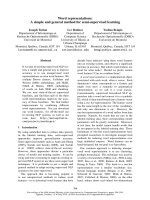
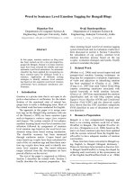
Figure 2: Classification result of LP on two-moon pattern
dataset. (a) Minimum spanning tree of this dataset. The conver-
gence process of LP algorithm with t varying from 1 to 100 is
shown from (b) to (f).
labeled. The distance metric is Euclidian distance.
We can see that the points in one moon should be
more similar to each other than the points across the
moons.
Figure 1(b) shows the classification result of
SVM. Vertical line denotes classification hyper-
plane, which has the maximum separating margin
with respect to the labeled points in two classes. We

can see that SVM does not work well when labeled
data can not reveal the structure (two moon pattern)
in each class. The reason is that the classification
hyperplane was learned only from labeled data. In
other words, the coherent structure (two-moon pat-
tern) in unlabeled data was not explored when infer-
ring class boundary.
Figure 1(c) shows bootstrapping procedure using
kNN (k=1) as base classifier with user-specified pa-
rameter b = 1 (the number of added examples from
unlabeled data into classified data for each class in
each iteration). Termination condition is that the dis-
tance between labeled and unlabeled points is more
than inter-class distance (the distance between A
0
and B
0
). Each arrow in Figure 1(c) represents
one classification operation in each iteration for each
class. After eight iterations, A
1
∼ A
8
were tagged
397
as +1, and B
1
∼ B
8
were tagged as −1, while

A
9
∼ A
10
and B
9
∼ B
10
were still untagged. Then
at the ninth iteration, A
9
was tagged as +1 since the
label of A
9
was determined only by labeled points in
kNN model: A
9
is closer to any point in {A
0
∼ A
8
}
than to any point in {B
0
∼ B
8
}, regardless of the
intrinsic structure in data: A
9
∼ A

10
and B
9
∼ B
10
are closer to points in lower moon than to points in
upper moon. In other words, bootstrapping method
uses the unlabeled data under a local consistency
based strategy. This is the reason that two points A
9
and A
10
are misclassified (shown in Figure 1(c)).
From above analysis we see that both SVM and
bootstrapping are based on a local consistency as-
sumption.
Finally we ran LP on a connected graph-minimum
spanning tree generated for this dataset, shown in
Figure 2(a). A, B, C represent three points, and
the edge A − B connects the two moons. Figure
2(b)- 2(f) shows the convergence process of LP with
t increasing from 1 to 100. When t = 1, label in-
formation of labeled data was pushed to only nearby
points. After seven iteration steps (t = 7), point B
in upper moon was misclassified as −1 since it first
received label information from point A through the
edge connecting two moons. After another three it-
eration steps (t=10), this misclassified point was re-
tagged as +1. The reason of this self-correcting be-
havior is that with the push of label information from

nearby points, the value of Y
B,+1
became higher
than Y
B,−1
. In other words, the weight of edge
B − C is larger than that of edge B − A, which
makes it easier for +1 label of point C to travel to
point B. Finally, when t ≥ 12 LP converged to a
fixed point, which achieved the ideal classification
result.
4 Experiments and Results
4.1 Experiment Design
For empirical comparison with SVM and bootstrap-
ping, we evaluated LP on widely used benchmark
corpora - “interest”, “line”
1
and the data in English
lexical sample task of SENSEVAL-3 (including all
57 English words )
2
.
1
Available at />2
Available at />Table 1: The upper two tables summarize accuracies (aver-
aged over 20 trials) and paired t-test results of SVM and LP on
SENSEVAL-3 corpus with percentage of training set increasing
from 1% to 100%. The lower table lists the official result of
baseline (using most frequent sense heuristics) and top 3 sys-
tems in ELS task of SENSEVAL-3.

Percentage SVM LP
cosine
LP
JS
1% 24.9±2.7% 27.5±1.1% 28.1±1.1%
10% 53.4±1.1% 54.4±1.2% 54.9±1.1%
25% 62.3±0.7% 62.3±0.7% 63.3±0.9%
50% 66.6±0.5% 65.7±0.5% 66.9±0.6%
75% 68.7±0.4% 67.3±0.4% 68.7±0.3%
100% 69.7% 68.4% 70.3%
Percentage SVM vs. LP
cosine
SVM vs. LP
JS
p-value Sign. p-value Sign.
1% 8.7e-004 ≪ 8.5e-005 ≪
10% 1.9e-006 ≪ 1.0e-008 ≪
25% 9.2e-001 ∼ 3.0e-006 ≪
50% 1.9e-006 ≫ 6.2e-002 ∼
75% 7.4e-013 ≫ 7.1e-001 ∼
100% - - - -
Systems Baseline htsa3 IRST-Kernels nusels
Accuracy 55.2% 72.9% 72.6% 72.4%
We used three types of features to capture con-
textual information: part-of-speech of neighboring
words with position information, unordered sin-
gle words in topical context, and local collocations
(as same as the feature set used in (Lee and Ng,
2002) except that we did not use syntactic relations).
For SVM, we did not perform feature selection on

SENSEVAL-3 data since feature selection deterio-
rates its performance (Lee and Ng, 2002). When
running LP on the three datasets, we removed the
features with occurrence frequency (counted in both
training set and test set) less than 3 times.
We investigated two distance measures for LP: co-
sine similarity and Jensen-Shannon (JS) divergence
(Lin, 1991).
For the three datasets, we constructed connected
graphs following (Zhu et al., 2003): two instances
u, v will be connected by an edge if u is among v’s
k nearest neighbors, or if v is among u’s k nearest
neighbors as measured by cosine or JS distance mea-
sure. For “interest” and “line” corpora, k is 10 (fol-
lowing (Zhu et al., 2003)), while for SENSEVAL-3
data, k is 5 since the size of dataset for each word
in SENSEVAL-3 is much less than that of “interest”
and “line” datasets.
398
4.2 Experiment 1: LP vs. SVM
In this experiment, we evaluated LP and SVM
3
on the data of English lexical sample task in
SENSEVAL-3. We used l examples from training
set as labeled data, and the remaining training ex-
amples and all the test examples as unlabeled data.
For each labeled set size l, we performed 20 trials.
In each trial, we randomly sampled l labeled exam-
ples for each word from training set. If any sense
was absent from the sampled labeled set, we redid

the sampling. We conducted experiments with dif-
ferent values of l, including 1% × N
w,train
, 10% ×
N
w,train
, 25% × N
w,train
, 50% × N
w,train
, 75% ×
N
w,train
, 100% × N
w,train
(N
w,train
is the number
of examples in training set of word w). SVM and LP
were evaluated using accuracy
4
(fine-grained score)
on test set of SENSEVAL-3.
We conducted paired t-test on the accuracy fig-
ures for each value of l. Paired t-test is not run when
percentage= 100%, since there is only one paired
accuracy figure. Paired t-test is usually used to esti-
mate the difference in means between normal pop-
ulations based on a set of random paired observa-
tions. {≪, ≫}, {<, >}, and ∼ correspond to p-

value ≤ 0.01, (0.01, 0.05], and > 0.05 respectively.
≪ (or ≫) means that the performance of LP is sig-
nificantly better (or significantly worse) than SVM.
< (or >) means that the performance of LP is better
(or worse) than SVM. ∼ means that the performance
of LP is almost as same as SVM.
Table 1 reports the average accuracies and paired
t-test results of SVM and LP with different sizes
of labled data. It also lists the official results of
baseline method and top 3 systems in ELS task of
SENSEVAL-3.
From Table 1, we see that with small labeled
dataset (percentage of labeled data ≤ 10%), LP per-
forms significantly better than SVM. When the per-
centage of labeled data increases from 50% to 75%,
the performance of LP
JS
and SVM become almost
same, while LP
cosine
performs significantly worse
than SVM.
3
we used linear SV M
light
, available at
/>4
If there are multiple sense tags for an instance in training
set or test set, then only the first tag is considered as correct
answer. Furthermore, if the answer of the instance in test set is

“U”, then this instance will be removed from test set.
Table 2: Accuracies from (Li and Li, 2004) and average ac-
curacies of LP with c × b labeled examples on “interest” and
“line” corpora. Major is a baseline method in which they al-
ways choose the most frequent sense. MB-D denotes monolin-
gual bootstrapping with decision list as base classifier, MB-B
represents monolingual bootstrapping with ensemble of Naive
Bayes as base classifier, and BB is bilingual bootstrapping with
ensemble of Naive Bayes as base classifier.
Ambiguous Accuracies from (Li and Li, 2004)
words Major MB-D MB-B BB
interest 54.6% 54.7% 69.3% 75.5%
line 53.5% 55.6% 54.1% 62.7%
Ambiguous Our results
words #labeled examples LP
cosine
LP
JS
interest 4×15=60 80.2±2.0% 79.8±2.0%
line 6×15=90 60.3±4.5% 59.4±3.9%
4.3 Experiment 2: LP vs. Bootstrapping
Li and Li (2004) used “interest” and “line” corpora
as test data. For the word “interest”, they used its
four major senses. For comparison with their re-
sults, we took reduced “interest” corpus (constructed
by retaining four major senses) and complete “line”
corpus as evaluation data. In their algorithm, c is
the number of senses of ambiguous word, and b
(b = 15) is the number of examples added into clas-
sified data for each class in each iteration of boot-

strapping. c × b can be considered as the size of
initial labeled data in their bootstrapping algorithm.
We ran LP with 20 trials on reduced “interest” cor-
pus and complete “line” corpus. In each trial, we
randomly sampled b labeled examples for each sense
of “interest” or “line” as labeled data. The rest
served as both unlabeled data and test data.
Table 2 summarizes the average accuracies of LP
on the two corpora. It also lists the accuracies of
monolingual bootstrapping algorithm (MB), bilin-
gual bootstrapping algorithm (BB) on “interest” and
“line” corpora. We can see that LP performs much
better than MB-D and MB-B on both “interest” and
“line” corpora, while the performance of LP is com-
parable to BB on these two corpora.
4.4 An Example: Word “use”
For investigating the reason for LP to outperform
SVM and monolingual bootstrapping, we used the
data of word “use” in English lexical sample task of
SENSEVAL-3 as an example (totally 26 examples
in training set and 14 examples in test set). For data
399
−0.4 −0.2 0 0.2 0.4 0.6
−0.5
0
0.5
−0.4 −0.2 0 0.2 0.4 0.6
−0.5
0
0.5

−0.4 −0.2 0 0.2 0.4 0.6
−0.5
0
0.5
−0.4 −0.2 0 0.2 0.4 0.6
−0.5
0
0.5
−0.4 −0.2 0 0.2 0.4 0.6
−0.5
0
0.5
−0.4 −0.2 0 0.2 0.4 0.6
−0.5
0
0.5
(a) Initial Setting
(b) Ground−truth
(c) SVM
(d) Bootstrapping
(e) Bootstrapping
(f) LP
B
A
C
Figure 3: Comparison of sense disambiguation results be-
tween SVM, monolingual bootstrapping and LP on word “use”.
(a) only one labeled example for each sense of word “use”
as training data before sense disambiguation (◦ and ⊲ denote
the unlabeled examples in SENSEVAL-3 training set and test

set respectively, and other five symbols (+, ×, △, ⋄, and ∇)
represent the labeled examples with different sense tags sam-
pled from SENSEVAL-3 training set.), (b) ground-truth re-
sult, (c) classification result on SENSEVAL-3 test set by SVM
(accuracy=
3
14
= 21.4%), (d) classified data after bootstrap-
ping, (e) classification result on SENSEVAL-3 training set and
test set by 1NN (accuracy=
6
14
= 42.9% ), (f) classifica-
tion result on SENSEVAL-3 training set and test set by LP
(accuracy=
10
14
= 71.4% ).
visualization, we conducted unsupervised nonlinear
dimensionality reduction
5
on these 40 feature vec-
tors with 210 dimensions. Figure 3 (a) shows the
dimensionality reduced vectors in two-dimensional
space. We randomly sampled only one labeled ex-
ample for each sense of word “use” as labeled data.
The remaining data in training set and test set served
as unlabeled data for bootstrapping and LP. All of
these three algorithms are evaluated using accuracy
on test set.

From Figure 3(c) we can see that SVM misclassi-
5
We used Isomap to perform dimensionality reduction by
computing two-dimensional, 39-nearest-neighbor-preserving
embedding of 210-dimensional input. Isomap is available at
/>fied many examples from class + into class × since
using only features occurring in training set can not
reveal the intrinsic structure in full dataset.
For comparison, we implemented monolingual
bootstrapping with kNN (k=1) as base classifier.
The parameter b is set as 1. Only b unlabeled ex-
amples nearest to labeled examples and with the
distance less than d
inter−class
(the minimum dis-
tance between labeled examples with different sense
tags) will be added into classified data in each itera-
tion till no such unlabeled examples can be found.
Firstly we ran this monolingual bootstrapping on
this dataset to augment initial labeled data. The re-
sulting classified data is shown in Figure 3 (d). Then
a 1NN model was learned on this classified data and
we used this model to perform classification on the
remaining unlabeled data. Figure 3 (e) reports the
final classification result by this 1NN model. We can
see that bootstrapping does not perform well since it
is susceptible to small noise in dataset. For example,
in Figure 3 (d), the unlabeled example B
6
happened

to be closest to labeled example A, then 1NN model
tagged example B with label ⋄. But the correct label
of B should be + as shown in Figure 3 (b). This
error caused misclassification of other unlabeled ex-
amples that should have label +.
In LP, the label information of example C can
travel to B through unlabeled data. Then example A
will compete with C and other unlabeled examples
around B when determining the label of B. In other
words, the labels of unlabeled examples are deter-
mined not only by nearby labeled examples, but also
by nearby unlabeled examples. Using this classifi-
cation strategy achieves better performance than the
local consistency based strategy adopted by SVM
and bootstrapping.
4.5 Experiment 3: LP
cosine
vs. LP
JS
Table 3 summarizes the performance comparison
between LP
cosine
and LP
JS
on three datasets. We
can see that on SENSEVAL-3 corpus, LP
JS
per-
6
In the two-dimensional space, example B is not the closest

example to A. The reason is that: (1) A is not close to most
of nearby examples around B, and B is not close to most of
nearby examples around A; (2) we used Isomap to maximally
preserve the neighborhood information between any example
and all other examples, which caused the loss of neighborhood
information between a few example pairs for obtaining a glob-
ally optimal solution.
400
Table 3: Performance comparison between LP
cosine
and
LP
JS
and the results of three model selection criteria are re-
ported in following two tables. In the lower table, < (or >)
means that the average value of function H(Q
cosine
) is lower
(or higher) than H(Q
JS
), and it will result in selecting cosine
(or JS) as distance measure. Q
cosine
(or Q
JS
) represents a ma-
trix using cosine similarity (or JS divergence).
√
and × denote
correct and wrong prediction results respectively, while ◦ means

that any prediction is acceptable.
LP
cosine
vs. LP
JS
Data p-value Significance
SENSEVAL-3 (1%) 1.1e-003 ≪
SENSEVAL-3 (10%) 8.9e-005 ≪
SENSEVAL-3 (25%) 9.0e-009 ≪
SENSEVAL-3 (50%) 3.2e-010 ≪
SENSEVAL-3 (75%) 7.7e-013 ≪
SENSEVAL-3 (100%) - -
interest 3.3e-002 >
line 8.1e-002 ∼
H(D ) H(W ) H(Y
U
)
Data cos. vs. JS cos. vs. JS cos. vs. JS
SENSEVAL-3 (1%) > (
√
) > (
√
) < (×)
SENSEVAL-3 (10%) < (×) > (
√
) < (×)
SENSEVAL-3 (25%) < (×) > (
√
) < (×)
SENSEVAL-3 (50%) > (

√
) > (
√
) > (
√
)
SENSEVAL-3 (75%) > (
√
) > (
√
) > (
√
)
SENSEVAL-3 (100%) < (◦) > (◦) < (◦)
interest < (
√
) > (×) < (
√
)
line > (◦) > (◦) > (◦)
forms significantly better than LP
cosine
, but their
performance is almost comparable on “interest” and
“line” corpora. This observation motivates us to au-
tomatically select a distance measure that will boost
the performance of LP on a given dataset.
Cross-validation on labeled data is not feasi-
ble due to the setting of semi-supervised learning
(l ≪ u). In (Zhu and Ghahramani, 2002; Zhu et

al., 2003), they suggested a label entropy criterion
H(Y
U
) for model selection, where Y is the label
matrix learned by their semi-supervised algorithms.
The intuition behind their method is that good para-
meters should result in confident labeling. Entropy
on matrix W (H(W )) is a commonly used measure
for unsupervised feature selection (Dash and Liu,
2000), which can be considered here. Another pos-
sible criterion for model selection is to measure the
entropy of c × c inter-class distance matrix D cal-
culated on labeled data (denoted as H(D)), where
D
i,j
represents the average distance between the i-
th class and the j-th class. We will investigate three
criteria, H(D), H(W ) and H(Y
U
), for model se-
lection. The distance measure can be automatically
selected by minimizing the average value of function
H(D), H(W ) or H(Y
U
) over 20 trials.
Let Q be the M × N matrix. Function H(Q) can
measure the entropy of matrix Q, which is defined
as (Dash and Liu, 2000):
S
i,j

= exp (−α ∗Q
i,j
), (1)
H(Q) = −
M

i=1
N

j=1
(S
i,j
log S
i,j
+ (1 − S
i,j
) log (1 − S
i,j
)),
(2)
where α is positive constant. The possible value of α
is −
ln 0.5
¯
I
, where
¯
I =
1
MN


i,j
Q
i,j
. S is introduced
for normalization of matrix Q. For SENSEVAL-
3 data, we calculated an overall average score of
H(Q) by

w
N
w,test

w
N
w,test
H(Q
w
). N
w,test
is the
number of examples in test set of word w. H(D),
H(W ) and H(Y
U
) can be obtained by replacing Q
with D, W and Y
U
respectively.
Table 3 reports the automatic prediction results
of these three criteria.

From Table 3, we can see that using H(W )
can consistently select the optimal distance measure
when the performance gap between LP
cosine
and
LP
JS
is very large (denoted by ≪ or ≫). But H(D)
and H(Y
U
) fail to find the optimal distance measure
when only very few labeled examples are available
(percentage of labeled data ≤ 10%).
H(W ) measures the separability of matrix W .
Higher value of H(W ) means that distance mea-
sure decreases the separability of examples in full
dataset. Then the boundary between clusters is ob-
scured, which makes it difficult for LP to locate this
boundary. Therefore higher value of H(W ) results
in worse performance of LP.
When labeled dataset is small, the distances be-
tween classes can not be reliably estimated, which
results in unreliable indication of the separability
of examples in full dataset. This is the reason that
H(D) performs poorly on SENSEVAL-3 corpus
when the percentage of labeled data is less than 25%.
For H(Y
U
), small labeled dataset can not reveal
intrinsic structure in data, which may bias the esti-

mation of Y
U
. Then labeling confidence (H(Y
U
))
can not properly indicate the performance of LP.
This may interpret the poor performance of H(Y
U
)
on SENSEVAL-3 data when percentage ≤ 25%.
401
5 Conclusion
In this paper we have investigated a label propaga-
tion based semi-supervised learning algorithm for
WSD, which fully realizes a global consistency as-
sumption: similar examples should have similar la-
bels. In learning process, the labels of unlabeled ex-
amples are determined not only by nearby labeled
examples, but also by nearby unlabeled examples.
Compared with semi-supervised WSD methods in
the first and second categories, our corpus based
method does not need external resources, includ-
ing WordNet, bilingual lexicon, aligned parallel cor-
pora. Our analysis and experimental results demon-
strate the potential of this cluster assumption based
algorithm. It achieves better performance than SVM
when only very few labeled examples are avail-
able, and its performance is also better than mono-
lingual bootstrapping and comparable to bilingual
bootstrapping. Finally we suggest an entropy based

method to automatically identify a distance measure
that can boost the performance of LP algorithm on a
given dataset.
It has been shown that one sense per discourse
property can improve the performance of bootstrap-
ping algorithm (Li and Li, 2004; Yarowsky, 1995).
This heuristics can be integrated into LP algorithm
by setting weight W
i,j
= 1 if the i-th and j-th in-
stances are in the same discourse.
In the future we may extend the evaluation of LP
algorithm and related cluster assumption based al-
gorithms using more benchmark data for WSD. An-
other direction is to use feature clustering technique
to deal with data sparseness and noisy feature prob-
lem.
Acknowledgements We would like to thank
anonymous reviewers for their helpful comments.
Z.Y. Niu is supported by A*STAR Graduate Schol-
arship.
References
Belkin, M., & Niyogi, P 2002. Using Manifold Structure for Partially Labeled
Classification. NIPS 15.
Blum, A., Lafferty, J., Rwebangira, R., & Reddy, R 2004. Semi-Supervised
Learning Using Randomized Mincuts. ICML-2004.
Brown P., Stephen, D.P., Vincent, D.P., & Robert, Mercer 1991. Word Sense
Disambiguation Using Statistical Methods. ACL-1991.
Chapelle, O., Weston, J., & Sch¨olkopf, B. 2002. Cluster Kernels for Semi-
supervised Learning. NIPS 15.

Dagan, I. & Itai A 1994. Word Sense Disambiguation Using A Second Lan-
guage Monolingual Corpus. Computational Linguistics, Vol. 20(4), pp. 563-
596.
Dash, M., & Liu, H 2000. Feature Selection for Clustering. PAKDD(pp. 110–
121).
Diab, M., & Resnik. P 2002. An Unsupervised Method for Word Sense Tagging
Using Parallel Corpora. ACL-2002(pp. 255–262).
Hearst, M 1991. Noun Homograph Disambiguation using Local Context in
Large Text Corpora. Proceedings of the 7th Annual Conference of the UW
Centre for the New OED and Text Research: Using Corpora, 24:1, 1–41.
Karov, Y. & Edelman, S 1998. Similarity-Based Word Sense Disambiguation.
Computational Linguistics, 24(1): 41-59.
Leacock, C., Miller, G.A. & Chodorow, M 1998. Using Corpus Statistics and
WordNet Relations for Sense Identification. Computational Linguistics, 24:1,
147–165.
Lee, Y.K. & Ng, H.T 2002. An Empirical Evaluation of Knowledge Sources and
Learning Algorithms for Word Sense Disambiguation. EMNLP-2002, (pp.
41-48).
Lesk M 1986. Automated Word Sense Disambiguation Using Machine Read-
able Dictionaries: How to Tell a Pine Cone from an Ice Cream Cone. Pro-
ceedings of the ACM SIGDOC Conference.
Li, H. & Li, C 2004. Word Translation Disambiguation Using Bilingual Boot-
strapping. Computational Linguistics, 30(1), 1-22.
Lin, D.K 1997. Using Syntactic Dependency as Local Context to Resolve Word
Sense Ambiguity. ACL-1997.
Lin, J. 1991. Divergence Measures Based on the Shannon Entropy. IEEE Trans-
actions on Information Theory, 37:1, 145–150.
McCarthy, D., Koeling, R., Weeds, J., & Carroll, J 2004. Finding Predominant
Word Senses in Untagged Text. ACL-2004.
Mihalcea R 2004. Co-training and Self-training for Word Sense Disambigua-

tion. CoNLL-2004.
Mihalcea R., Chklovski, T., & Kilgariff, A 2004. The SENSEVAL-3 English
Lexical Sample Task. SENSEVAL-2004.
Ng, H.T., Wang, B., & Chan, Y.S 2003. Exploiting Parallel Texts for Word
Sense Disambiguation: An Empirical Study. ACL-2003, pp. 455-462.
Park, S.B., Zhang, B.T., & Kim, Y.T 2000. Word Sense Disambiguation by
Learning from Unlabeled Data. ACL-2000.
Sch¨utze, H 1998. Automatic Word Sense Discrimination. Computational Lin-
guistics, 24:1, 97–123.
Seo, H.C., Chung, H.J., Rim, H.C., Myaeng. S.H., & Kim, S.H 2004. Unsu-
pervised Word Sense Disambiguation Using WordNet Relatives. Computer,
Speech and Language, 18:3, 253–273.
Szummer, M., & Jaakkola, T 2001. Partially Labeled Classification with Markov
Random Walks. NIPS 14.
Yarowsky, D 1995. Unsupervised Word Sense Disambiguation Rivaling Super-
vised Methods. ACL-1995, pp. 189-196.
Yarowsky, D 1992. Word Sense Disambiguation Using Statistical Models of
Roget’s Categories Trained on Large Corpora. COLING-1992, pp. 454-460.
Zhu, X. & Ghahramani, Z 2002. Learning from Labeled and Unlabeled Data
with Label Propagation. CMU CALD tech report CMU-CALD-02-107.
Zhu, X., Ghahramani, Z., & Lafferty, J 2003. Semi-Supervised Learning Using
Gaussian Fields and Harmonic Functions. ICML-2003.
402