Báo cáo khoa học: "Centrality Measures in Text Mining: Prediction of Noun " docx
Bạn đang xem bản rút gọn của tài liệu. Xem và tải ngay bản đầy đủ của tài liệu tại đây (93.77 KB, 6 trang )
Proceedings of the ACL Student Research Workshop, pages 103–108,
Ann Arbor, Michigan, June 2005.
c
2005 Association for Computational Linguistics
Centrality Measures in Text Mining:
Prediction of Noun Phrases that Appear in Abstracts
Zhuli Xie
Department of Computer Science
University of Illinois at Chicago
Chicago, IL 60607, U. S. A
Abstract
In this paper, we study different centrality
measures being used in predicting noun
phrases appearing in the abstracts of sci-
entific articles. Our experimental results
show that centrality measures improve the
accuracy of the prediction in terms of
both precision and recall. We also found
that the method of constructing Noun
Phrase Network significantly influences
the accuracy when using the centrality
heuristics itself, but is negligible when it
is used together with other text features in
decision trees.
1 Introduction
Research on text summarization, information re-
trieval, and information extraction often faces the
question of how to determine which words are
more significant than others in text. Normally we
only consider content words, i.e., the open class
words. Non-content words or stop words, which
are called function words in natural language proc-
essing, do not convey semantics so that they are
excluded although they sometimes appear more
frequently than content words. A content word is
usually defined as a term, although a term can also
be a phrase. Its significance is often indicated by
Term Frequency (TF) and Inverse Document Fre-
quency (IDF). The usage of TF comes from “the
simple notion that terms which occur frequently in
a document may reflect its meaning more strongly
than terms that occur less frequently” (Jurafsky
and Martin, 2000). On the contrary, IDF assigns
smaller weights to terms which are contained in
more documents. That is simply because “the more
documents having the term, the less useful the term
is in discriminating those documents having it
from those not having it” (Yu and Meng, 1998).
TF and IDF also find their usage in automatic
text summarization. In this circumstance, TF is
used individually more often than together with
IDF, since the term is not used to distinguish a
document from another. Automatic text summari-
zation seeks a way of producing a text which is
much shorter than the document(s) to be summa-
rized, and can serve as a surrogate for full-text.
Thus, for extractive summaries, i.e., summaries
composed of original sentences from the text to be
summarized, we try to find those terms which are
more likely to be included in the summary.
The overall goal of our research is to build a
machine learning framework for automatic text
summarization. This framework will learn the rela-
tionship between text documents and their corre-
sponding abstracts written by human. At the
current stage the framework tries to generate a sen-
tence ranking function and use it to produce extrac-
tive summaries. It is important to find a set of
features which represent most information in a sen-
tence and hence the machine learning mechanism
can work on it to produce a ranking function. The
next stage in our research will be to use the frame-
work to generate abstractive summaries, i.e. sum-
maries which do not use sentences from the input
text verbatim. Therefore, it is important to know
what terms should be included in the summary.
In this paper we present the approach of using
social network analysis technique to find terms,
specifically noun phrases (NPs) in our experi-
ments, which occur in the human-written abstracts.
We show that centrality measures increase the pre-
diction accuracy. Two ways of constructing noun
103
phrase network are compared. Conclusions and
future work are discussed at the end.
2 Centrality Measures
Social network analysis studies linkages among
social entities and the implications of these link-
ages. The social entities are called actors. A social
network is composed of a set of actors and the rela-
tion or relations defined on them (Wasserman and
Faust, 1994). Graph theory has been used in social
network analysis to identify those actors who im-
pose more influence upon a social network. A so-
cial network can be represented by a graph with
the actors denoted by the nodes and the relations
by the edges or links. To determine which actors
are prominent, a measure called centrality is intro-
duced. In practice, four types of centrality are often
used.
Degree centrality measures how many direct
connections a node has to other nodes in a net-
work. Since this measure depends on the size of
the network, a standardized version is used when it
is necessary to compare the centrality across net-
works of different sizes.
DegreeCentrality(n
i
) = d(n
i
)/(u-1),
where d(n
i
) is the degree of node i in a network
and u is the number of nodes in that network.
Closeness centrality focuses on the distances an
actor is from all other nodes in the network.
∑
u
iij
j=1
ClosenessCentrality(n )= (u- 1) d(n ,n ),
where d(n
i
, n
j
) is the shortest distance between
node
i and j.
Betweenness centrality emphasizes that for an
actor to be central, it must reside on many ge-
odesics of other nodes so that it can control the
interactions between them.
∑
j
ki jk
j<k
i
g(n)/g
BetweennessCentrality(n )=
(u- 1)(u- 2)/ 2
,
where
g
jk
is the number of geodesics linking node j
and
k, g
jk
(n
i
) is the number of geodesics linking the
two nodes that contain node
i.
Betweenness centrality is widely used because
of its generality. This measure assumes that infor-
mation flow between two nodes will be on the ge-
odesics between them. Nevertheless, “It is quite
possible that information will take a more circui-
tous route either by random communication or [by
being] channeled through many intermediaries in
order to 'hide' or 'shield' information”. (Stephenson
and Zelen, 1989).
Stephenson and Zelen (1989) developed infor-
mation centrality which generalizes betweenness
centrality. It focuses on the information contained
in all paths originating with a specific actor. The
calculation for information centrality of a node is
in the Appendix.
Recently centrality measures have started to
gain attention from researchers in text processing.
Corman et al. (2002) use vectors, which consist of
NPs, to represent texts and hence analyze mutual
relevance of two texts. The values of the elements
in a vector are determined by the betweenness cen-
trality of the NPs in a text being analyzed. Erkan
and Radev (2004) use the PageRank method,
which is the application of centrality concept to the
Web, to determine central sentences in a cluster for
summarization. Vanderwende et al. (2004) also use
the PageRank method to pick prominent triples, i.e.
(node i, relation, node j), and then use the triples to
generate event-centric summaries.
3 NP Networks
To construct a network for NPs in a text, we try
two ways of modeling the relation between them.
One is at the sentence level: if two noun phrases
can be sequentially parsed out from a sentence, a
link is added between them. The other way is at the
document level: we simply add a link to every pair
of noun phrases which are parsed out in succes-
sion. The difference between the two ways is that
the network constructed at the sentence level ig-
nores the existence of certain connections between
sentences.
We process a text document in four steps.
First, the text is tokenized and stored into an in-
ternal representation with structural information.
Second, the tokenized text is tagged by the Brill
tagging algorithm POS tagger.
1
Third, the NPs in a text document are parsed ac-
cording to 35 parsing rules as shown in Figure 1. If
a new noun phrase is found, a new node is formed
and added to the network. If the noun phrase al-
ready exists in the network, the node containing it
will be identified. A link will be added between
two nodes if they are parsed out sequentially for
1
The POS tagger we used can be obtained from
/>
104
the network formed at the document level, or se-
quentially in the same sentence for the network
formed at the sentence level.
Finally, after the text document has been proc-
essed, the centrality of each node in the network is
updated.
4 Predicting NPs Occurring in Abstracts
In this paper, we refer the NPs occur both in a text
document and its corresponding abstract as Co-
occurring NPs (CNPs).
4.1 CMP-LG Corpus
In our experiment, a corpus of 183 documents was
used. The documents are from the Computation
and Language collection and have been marked in
XML with tags providing basic information about
the document such as title, author, abstract, body,
sections, etc. This corpus is a part of the TIPSTER
Text Summarization Evaluation Conference
(SUMMAC) effort acting as a general resource to
the information retrieval, extraction and summari-
zation communities. We excluded five documents
from this corpus which do not have abstracts.
4.2 Using Noun Phrase Centrality Heuristics
We assume that a noun phrase with high centrality
is more likely to be a central topic being addressed
in a document than one with low centrality. Given
this assumption, we performed an experiment, in
which the NPs with highest centralities are re-
trieved and compared with the actual NPs in the
abstracts. To evaluate this method, we use Preci-
sion, which measures the fraction of true CNPs in
all predicted CNPs, and Recall, which measures
the fraction of correctly predicted CNPs in all
CNPs.
After establishing the NP network for a docu-
ment and ranking the nodes according to their cen-
tralities, we must decide how many NPs should be
retrieved. This number should not be too big; oth-
erwise the Precision value will be very low, al-
though the Recall will be higher. If this number is
very small, the Recall will decrease correspond-
ingly. We adopted a compound metric - F-
measure, to balance the selection:
Based on our study of 178 documents in the
CMP-LG corpus, we find that the number of CNPs
is roughly proportional to the number of NPs in the
abstract. We obtain a linear regression model for
the data shown in Figure 2 and use this model to
calculate the number of nodes we should retrieve
from the NP network, given the number of NPs in
the abstract known a priori:
One could argue that the number of abstract NPs is
unknown a priori and thus the proposed method is
of limited use. However, the user can provide an
estimate based on the desired number of words in
the summary. Here we can adopt the same way of
asking the user to provide a limit for the NPs in the
summary. We used the actual number of NPs the
author used in his/her abstract in our experiment.
Figure 2. Scatter Plot of CNPs
0
5
10
15
20
25
30
35
40
0 10203040506070
Number of NPs in Abstract
Number of CNPs
Our experiment results are shown in Figure 3(a)
and 3(b). In 3(a) the NP network is formed at sen-
NX > CD
NX > CD NNS
NX > NN
NX > NN NN
NX > NN NNS
NX > NN NNS NN
NX > NNP
NX > NNP CD
NX > NNP NNP
NX > NNP NNPS
NX > NNP NN
NX > NNP NNP NNP
NX > JJ NN
NX > JJ NNS
NX > JJ NN NNS
NX > PRP$ NNS
NX > PRP$ NN
NX > PRP$ NN NN
NX > NNS
NX > PRP
NX > WP$ NNS
NX > WDT
NX > EX
NX > WP
NX > DT JJ NN
NX > DT CD NNS
NX > DT VBG NN
NX > DT NNS
NX > DT NN
NX > DT NN NN
NX > DT NNP
NX > DT NNP NN
NX > DT NNP NNP
NX > DT NNP NNP NNP
NX >DT NNP NNP NN NN
Figure 1. NP Parsing Rules
F-measure=2*Precision*Recall/(Precision+Recall)
N
umbe
r
of Common NPs =
0.555 * Number of NPs in Abstrac
t
+ 2.435
105
tence level. In this way, it is possible the graph will
be composed of disconnected subgraphs. In such
case, we calculate the closeness centrality (cc),
betweenness centrality (bc), and the information
centrality (ic) within the subgraphs while the de-
gree centrality (dc) is still computed for the overall
graph. In 3(b), the network is constructed at the
document level. Therefore, it is guaranteed that
every node is reachable from all other node.
Figure 3(a) shows the simplest centrality meas-
ure dc performs best, with Precision, Recall, and F-
measure all greater than 0.2, which are twice of bc
and almost ten times of cc and ic.
In Figure 3(b), however, all four measures are
around 0.25 in all three evaluation metrics. This
result suggests to us that when we choose a cen-
trality to represent the prominence of a NP in the
text, not only does the kind of the centrality matter,
but also the way of forming the NP network.
Overall, the heuristic of using centrality itself
does not achieve impressive scores. We will see in
the next section that using decision trees is a much
better way to perform the predictions, when using
centrality together with other text features.
4.3 Using Decision Trees
We obtain the following features for all NPs in a
document from the CMP-LG corpus:
Position: the order of a NP appearing in the text,
normalized by the total number of NPs.
Article: three classes are defined for this attribute:
INDEfinite (contains a or an), DEFInite (contains
the), and NONE (all others).
Degree centrality: obtained from the NP network
Closeness centrality: obtained from the NP net-
work
Betweenness centrality: obtained from the NP
network
Information centrality: obtained from the NP
network
Head noun POS tag: a head noun is the last word
in the NP. Its POS tag is used here.
Proper name: whether the NP is a proper name,
by looking at the POS tags of all words in the NP.
Number: whether the NP is just one number.
Frequency: how many times a NP occurs in a text,
normalized by its maximum.
In abstract: whether the NP appears in the author-
provided abstract. This attribute is the target for the
decision trees to classify.
Figure 3(a). Centrality Heuristics
(Network at Sentence Level)
0
0.05
0.1
0.15
0.2
0.25
0.3
Precision Recall F-measure
dc
cc
bc
ic
Figure 3(b). Centrality Heuristics
(Network at Document Level)
0
0.05
0.1
0.15
0.2
0.25
0.3
Precision Recall F-measure
dc
cc
bc
ic
In order to learn which type of centrality meas-
ures helps to improve the accuracy of the predic-
tions, and to see whether centrality measures are
better than term frequency, we experiment with six
groups of feature sets and compare their perform-
ances. The six groups are:
All: including all features above.
DC: including only the degree centrality measure,
and other non-centrality measures except for Fre-
quency.
CC: same as DC except for using closeness cen-
trality instead of degree centrality.
BC: same as DC except for using betweenness
centrality instead of degree centrality.
IC: same as DC except for using information cen-
trality instead of degree centrality.
FQ: including Frequency and all other non-
centrality features.
The 178 documents have generated more than
100,000 training records. Among them only a very
small portion (2.6%) belongs to the positive class.
When using decision tree algorithm on such imbal-
anced attribute, it is very common that the class
with absolute advantages will be favored (Japko-
wicz, 2000; Kubat and Matwin, 1997). To reduce
106
Precision
0.817 0.816 0.795
0.809
0.767 0.787 0.732
0.762
0.774 0.795 0.769
0.779
Recall
0.971 0.984 0.96
0.972
0.791 0.866 0.8
0.819
0.651 0.696 0.639
0.662
F-measure
0.887 0.892 0.869
0.883
0.779 0.825 0.764
0.789
0.706 0.742 0.696
0.715
Precision
0.795 0.82 0.795
0.803
0.772 0.806 0.768
0.782
0.767 0.806 0.766
0.78
Recall
0.944 0.976 0.946
0.955
0.79 0.892 0.755
0.812
0.72 0.892 0.644
0.752
F-measure
0.863 0.891 0.864
0.873
0.781 0.846 0.761
0.796
0.743 0.846 0.698
0.763
Set 1Set 2Set 3
Mean
Set 1 Set 2 Set 3
Mean
Set 1Set 2Set 3
Mean
Precision
0.738 0.799 0.745
0.761
0.722 0.759 0.743
0.742
0.774 0.79 0.712
0.759
Recall
0.698 0.874 0.733
0.768
0.666 0.799 0.667
0.711
0.763 0.878 0.78
0.807
F-measure
0.716 0.835 0.737
0.763
0.693 0.779 0.702
0.724
0.768 0.831 0.744
0.781
Precision
0.767 0.799 0.75
0.772
0.756 0.798 0.759
0.771
0.734 0.794 0.74
0.756
Recall
0.672 0.814 0.666
0.717
0.769 0.916 0.72
0.802
0.728 0.886 0.707
0.774
F-measure
0.716 0.806 0.705
0.742
0.762 0.853 0.738
0.784
0.73 0.837 0.722
0.763
Set 1Set 2Set 3
Mean
Set 1 Set 2 Set 3
Mean
Set 1Set 2Set 3
Mean
CC
BC
Sentence
Level
Document
Level
All DC
Sentence
Level
Document
Level
IC F
Q
Table 1. Results for Using 6 Feature Sets with YaDT
the unfair preference, one way is to boost the weak
class, e.g., by replicating instances in the minority
class (Kubat and Matwin, 1997; Chawla et al.,
2000). In our experiments, the 178 documents
were arbitrarily divided into three roughly equal
groups, generating 36,157, 37,600, and 34,691 re-
cords, respectively. After class balancing, the re-
cords are increased to 40,109, 42,210, and 38,499.
The three data sets were then run through the deci-
sion tree algorithm YaDT (Yet another Decision
Tree builder), which is much more efficient than
C4.5 (Ruggieri, 2004),
2
with 10-fold cross valida-
tion.
The experiment results of using YaDT with
three data sets and six feature groups to predict the
CNPs are shown in Table 1. The mean values of
three metrics are also shown in Figure 4(a) and
4(b). Decision trees achieve much higher scores
compared with the scores obtained by using cen-
trality heuristics. Together with other text features,
DC, CC, BC, and IC obtain scores over 0.7 in all
three metric, which are comparable to the scores
obtained by using FQ. Moreover, when using all
the features, decision trees achieve over 0.8 in pre-
cision and over 0.95 in recall. F-measure is as high
as 0.88. To see whether F-measure of All is statis-
tically better than that of other settings, we run t-
tests to compare them using values of F-measure
obtained in the 10-fold cross-validation from the
three data sets. The results show the mean value of
F-measure of All is significantly higher (p-value
=0.000) than that of other settings.
Differently from the experiments that use centrality
heuristics by itself, almost no obvious distinctions
2
The YaDT software can be obtained from
/>
can be observed when comparing the performances
of YaDT with NP network formed in two ways.
5 Conclusions and Future work
We have studied four kinds of centrality measures
in order to identify prominent noun phrases in text
documents. Overall, the centrality heuristic itself
does not demonstrate its superiority. Among four
centrality measures, degree centrality performs the
best in the heuristic when the NP network is con-
structed at the sentence level, which indicates other
centrality measures obtained from the subgraphs
can not represent very well the prominence of the
NPs in the global NP network. When the NP net-
work is constructed at the document level, the dif-
ferences between the centrality measures become
negligible. However, networks formed at the
document level overlook the connections between
sentences as there is only one kind of link; on the
other hand, NP networks formed at the sentence
level ignore connections between sentences. We
plan to extend our study to construct NP networks
with weighted links. The key problem will be how
to determine the weights for links between two
NPs in the same sentence, in the same paragraph
but different sentences, and in different paragraphs.
We consider introducing the concept of entropy
from Information Theory to solve this problem.
In our experiments with YaDT, it seems the ways
of forming NP network are not critical. We learn
that, at least in this circumstance, the decision trees
algorithm is more robust than the centrality heuris-
tic. When using all features in YaDT, recall
reaches 0.95, which means the decision trees find
out 95% of CNPs in the abstracts from the text
documents, without increasing mistakes as the
107
Figure 4(a). Results with NP Network
Formed in Sentence Level
0.6
0.7
0.8
0.9
1
Precision Recall F-measure
All
DC
CC
BC
IC
FQ
Figure 4(b). Results with NP Network
Formed in Document Level
0.6
0.7
0.8
0.9
1
Precision Recall F-measure
All
DC
CC
BC
IC
FQ
precision is improved at the same time. Using all
features in YaDT achieves better results than using
centrality feature or frequency individually with
other features implies centrality features may cap-
ture somewhat different information from the text.
To make this research more robust, we will in-
clude reference resolution into our study. We will
also include centrality measures as sentence
features in producing extractive summaries.
References
N. Chawla, K. Bowyer, L. Hall, and W. P. Kegelmeyer.
2000. SMOTE: synthetic minority over-sampling
technique. In Proc. of the International Conference
on Knowledge Based Computer Systems, India.
S. Corman, T. Kuhn, R. McPhee, and K. Dooley. 2002.
Studying complex discursive systems: Centering
resonance analysis of organizational communication.
Human Communication Research, 28(2):157-206.
G. Erkan and D. R. Radev. 2004. The University of
Michigan at DUC 2004. In Document Understanding
Conference 2004, Boston, MA.
N. Japkowicz. 2000. The class imbalance problem: sig-
nificance and strategies. In Proc. of the 2000 Interna-
tional Conference on Artificial Intelligence.
D. Jurafsky and J. H. Martin. 2000. Speech and Lan-
guage Processing: An Introduction to Natural Lan-
guage Processing, Computational Linguistics, and
Speech Recognition. Prentice Hall, Upper Saddle
River, NJ.
M. Kubat and S. Matwin. 1997. Addressing the curse of
imbalanced data sets: one-sided sampling. In Proc. of
the Fourteenth International Conference on Machine
Learning, Morgan Kauffman, 179–186.
S. Ruggieri. 2004. YaDT: Yet another Decision Tree
builder. In Proc. of the 16th International Conference
on Tools with Artificial Intelligence (ICTAI 2004),
260-265. Boca Raton, FL
K. Stephenson and M. Zelen. 1989. Rethinking central-
ity: Methods and applications. Social Networks. 11:1-
37.
L. Vanderwende, M. Banko and A. Menezes. 2004.
Event-Centric Summary Generation. In Document
Understanding Conference 2004. Boston, MA.
S. Wasserman and K. Faust. 1994. Social Network
Analysis: Methods and applications. Cambridge
University Press.
C. T. Yu and W. Meng. 1998. Principles of Database
Query Processing for Advanced Applications. Mor-
gan Kaufmann Publishers, San Francisco, CA.
Appendix: Calculation of Information Cen-
trality
Consider a network with n points where every pair
of points is reachable. Define the
nn× matrix
()
ij
B
b
=
by:
0 if points and are incident
1 otherwise;
1 + degree of point
ij
ii
ij
b
bi
⎧
=
⎨
⎩
=
Define the matrix
1
()
ij
Cc B
−
==
. The value of I
ij
(the information in the combined path P
ij
) is given
explicitly by
1
(2)
ij ii jj ij
Iccc
−
=+−
.
We can write
11
1( 2) 2
nn
ij ii jj ij ii
jj
I
cc c ncT R
==
=+−=+−
∑∑
,
where
11
and
nn
j
jij
jj
Tc Rc
==
==
∑
∑
.
Therefore the centrality for point i can be explicitly
written as
1
2(2)/
i
ii ii
n
I
nc T R c T R n
==
+− + −
.
(Stephenson and Zelen 1989).
108