Báo cáo khoa học: "Discriminative Language Modeling with Conditional Random Fields and the Perceptron Algorithm" pptx

Discriminative Language Modeling with
Conditional Random Fields and the Perceptron Algorithm
Brian Roark Murat Saraclar
AT&T Labs - Research
{roark,murat}@research.att.com
Michael Collins Mark Johnson
MIT CSAIL Brown University
Mark
Abstract
This paper describes discriminative language modeling
for a large vocabulary speech recognition task. We con-
trast two parameter estimation methods: the perceptron
algorithm, and a method based on conditional random
fields (CRFs). The models are encoded as determin-
istic weighted finite state automata, and are applied by
intersecting the automata with word-lattices that are the
output from a baseline recognizer. The perceptron algo-
rithm has the benefit of automatically selecting a rela-
tively small feature set in just a couple of passes over the
training data. However, using the feature set output from
the perceptron algorithm (initialized with their weights),
CRF training provides an additional 0.5% reduction in
word error rate, for a total 1.8% absolute reduction from
the baseline of 39.2%.
1 Introduction
A crucial component of any speech recognizer is the lan-
guage model (LM), which assigns scores or probabilities
to candidate output strings in a speech recognizer. The
language model is used in combination with an acous-
tic model, to give an overall score to candidate word se-
quences that ranks them in order of probability or plau-

sibility.
A dominant approach in speech recognition has been
to use a “source-channel”, or “noisy-channel” model. In
this approach, language modeling is effectively framed
as density estimation: the language model’s task is to
define a distribution over the source – i.e., the possible
strings in the language. Markov (n-gram) models are of-
ten used for this task, whose parameters are optimized
to maximize the likelihood of a large amount of training
text. Recognition performance is a direct measure of the
effectiveness of a language model; an indirect measure
which is frequently proposed within these approaches is
the perplexity of the LM (i.e., the log probability it as-
signs to some held-out data set).
This paper explores alternative methods for language
modeling, which complement the source-channel ap-
proach through discriminatively trained models. Thelan-
guage models we describe do not attempt to estimate a
generative model P (w) over strings. Instead, they are
trained on acoustic sequences with their transcriptions,
in an attempt to directly optimize error-rate. Our work
builds on previous work on language modeling using the
perceptron algorithm, described in Roark et al. (2004).
In particular, we explore conditional random field meth-
ods, as an alternative training method to the perceptron.
We describe how these models can be trained over lat-
tices that are the output from a baseline recognizer. We
also give a number of experiments comparing the two ap-
proaches. The perceptron method gave a 1.3% absolute
improvement in recognition error on the Switchboard do-

main; the CRF methods we describe give a further gain,
the final absolute improvement being 1.8%.
A central issue we focus on concerns feature selection.
The number of distinct n-grams in our training data is
close to 45 million, and we show that CRF training con-
verges very slowly even when trained with a subset (of
size 12 million) of these features. Because of this, we ex-
plore methods for picking a small subset of the available
features.
1
The perceptron algorithm can be used as one
method for feature selection, selecting around 1.5 million
features in total. The CRF trained with this feature set,
and initialized with parameters from perceptron training,
converges much more quickly than other approaches, and
also gives the optimal performance on the held-out set.
We explore other approaches to feature selection, but find
that the perceptron-based approach gives the best results
in our experiments.
While we focus on n-gram models, we stress that our
methods are applicable to more general language mod-
eling features – for example, syntactic features, as ex-
plored in, e.g., Khudanpur and Wu (2000). We intend
to explore methods with new features in the future. Ex-
perimental results with n-gram models on 1000-best lists
show a very small drop in accuracy compared to the use
of lattices. This is encouraging, in that it suggests that
models with more flexible features than n-gram models,
which therefore cannot be efficiently used with lattices,
may not be unduly harmed by their restriction to n-best

lists.
1.1 Related Work
Large vocabulary ASR has benefitted from discrimina-
tive estimation of Hidden Markov Model (HMM) param-
eters in the form of Maximum Mutual Information Es-
timation (MMIE) or Conditional Maximum Likelihood
Estimation (CMLE). Woodland and Povey (2000) have
shown the effectiveness of lattice-based MMIE/CMLE in
challenging large scale ASR tasks such as Switchboard.
In fact, state-of-the-art acoustic modeling, as seen, for
example, at annual Switchboard evaluations, invariably
includes some kind of discriminative training.
Discriminative estimation of language models has also
been proposed in recent years. Jelinek (1995) suggested
an acoustic sensitive language model whose parameters
1
Note also that in addition to concerns about training time, a lan-
guage model with fewer features is likely to be considerably more effi-
cient when decoding new utterances.
are estimated by minimizing H(W |A), the expected un-
certainty of the spoken text W, given the acoustic se-
quence A. Stolcke and Weintraub (1998) experimented
with various discriminative approaches including MMIE
with mixed results. This work was followed up with
some success by Stolcke et al. (2000) where an “anti-
LM”, estimated from weighted N-best hypotheses of a
baseline ASR system, was used with a negative weight
in combination with the baseline LM. Chen et al. (2000)
presented a method based on changing the trigram counts
discriminatively, together with changing the lexicon to

add new words. Kuo et al. (2002) used the generalized
probabilistic descent algorithm to train relatively small
language models which attempt to minimize string error
rate on the DARPA Communicator task. Banerjee et al.
(2003) used a language model modification algorithm in
the context of a reading tutor that listens. Their algorithm
first uses a classifier to predict what effect each parame-
ter has on the error rate, and then modifies the parameters
to reduce the error rate based on this prediction.
2 Linear Models, the Perceptron
Algorithm, and Conditional Random
Fields
This section describes a general framework, global linear
models, and two parameter estimation methods within
the framework, the perceptron algorithm and a method
based on conditional random fields. The linear models
we describe are general enough to be applicable to a di-
verse range of NLP and speech tasks – this section gives
a general description of the approach. In the next section
of the paper we describe how global linear models can
be applied to speech recognition. In particular, we focus
on how the decoding and parameter estimation problems
can be implemented over lattices using finite-state tech-
niques.
2.1 Global linear models
We follow the framework outlined in Collins (2002;
2004). The task is to learn a mapping from inputs x ∈ X
to outputs y ∈ Y. We assume the following compo-
nents: (1) Training examples (x
i

, y
i
) for i = 1 . . . N.
(2) A function GEN which enumerates a set of candi-
dates GEN(x) for an input x. (3) A representation
Φ mapping each (x, y) ∈ X × Y to a feature vector
Φ(x, y) ∈ R
d
. (4) A parameter vector ¯α ∈ R
d
.
The components GEN, Φ and ¯α define a mapping
from an input x to an output F (x) through
F (x) = argmax
y∈GEN(x)
Φ(x, y) · ¯α (1)
where Φ(x, y) · ¯α is the inner product

s
α
s
Φ
s
(x, y).
The learning task is to set the parameter values ¯α using
the training examples as evidence. The decoding algo-
rithm is a method for searching for the y that maximizes
Eq. 1.
2.2 The Perceptron algorithm
We now turn to methods for training the parameters

¯α of the model, given a set of training examples
Inputs: Training examples (x
i
, y
i
)
Initialization: Set ¯α = 0
Algorithm:
For t = 1 . . . T, i = 1 . . . N
Calculate z
i
= argmax
z∈GEN(x
i
)
Φ(x
i
, z) · ¯α
If(z
i
= y
i
) then ¯α = ¯α + Φ(x
i
, y
i
) − Φ(x
i
, z
i

)
Output: Parameters ¯α
Figure 1: A variant of the perceptron algorithm.
(x
1
, y
1
) . . . (x
N
, y
N
). This section describes the per-
ceptron algorithm, which was previously applied to lan-
guage modeling in Roark et al. (2004). The next section
describes an alternative method, based on conditional
random fields.
The perceptron algorithm is shown in figure 1. At
each training example (x
i
, y
i
), the current best-scoring
hypothesis z
i
is found, and if it differs from the refer-
ence y
i
, then the cost of each feature
2
is increased by

the count of that feature in z
i
and decreased by the count
of that feature in y
i
. The features in the model are up-
dated, and the algorithm moves to the next utterance.
After each pass over the training data, performance on
a held-out data set is evaluated, and the parameterization
with the best performance on the held out set is what is
ultimately produced by the algorithm.
Following Collins (2002), we used the averaged pa-
rameters from the training algorithm in decoding held-
out and test examples in our experiments. Say ¯α
t
i
is the
parameter vector after the i’th example is processed on
the t’th pass through the data in the algorithm in fig-
ure 1. Then the averaged parameters ¯α
AV G
are defined
as ¯α
AV G
=

i,t
¯α
t
i

/N T. Freund and Schapire (1999)
originally proposed the averaged parameter method; it
was shown to give substantial improvements in accuracy
for tagging tasks in Collins (2002).
2.3 Conditional Random Fields
Conditional Random Fields have been applied to NLP
tasks such as parsing (Ratnaparkhi et al., 1994; Johnson
et al., 1999), and tagging or segmentation tasks (Lafferty
et al., 2001; Sha and Pereira, 2003; McCallum and Li,
2003; Pinto et al., 2003). CRFs use the parameters ¯α
to define a conditional distribution over the members of
GEN(x) for a given input x:
p
¯α
(y|x) =
1
Z(x, ¯α)
exp (Φ(x, y) · ¯α)
where Z(x, ¯α) =

y∈GEN(x)
exp (Φ(x, y) · ¯α) is a
normalization constant that depends on x and ¯α.
Given these definitions, the log-likelihood of the train-
ing data under parameters ¯α is
LL(¯α) =
N

i=1
log p

¯α
(y
i
|x
i
)
=
N

i=1
[Φ(x
i
, y
i
) · ¯α − log Z(x
i
, ¯α)] (2)
2
Note that here lattice weights are interpreted as costs, which
changes the sign in the algorithm presented in figure 1.
Following Johnson et al. (1999) and Lafferty et al.
(2001), we use a zero-mean Gaussian prior on the pa-
rameters resulting in the regularized objective function:
LL
R
(¯α) =
N

i=1
[Φ(x

i
, y
i
) · ¯α − log Z(x
i
, ¯α)] −
||¯α||
2
2σ
2
(3)
The value σ dictates the relative influence of the log-
likelihood term vs. the prior, and is typically estimated
using held-out data. The optimal parameters under this
criterion are ¯α
∗
= argmax
¯α
LL
R
(¯α).
We use a limited memory variable metric method
(Benson and Mor
´
e, 2002) to optimize LL
R
. There is a
general implementation of this method in the Tao/PETSc
software libraries (Balay et al., 2002; Benson et al.,
2002). This technique has been shown to be very effec-

tive in a variety of NLP tasks (Malouf, 2002; Wallach,
2002). The main interface between the optimizer and the
training data is a procedure which takes a parameter vec-
tor ¯α as input, and in turn returns LL
R
(¯α) as well as
the gradient of LL
R
at ¯α. The derivative of the objec-
tive function with respect to a parameter α
s
at parameter
values ¯α is
∂LL
R
∂α
s
=
N

i=1


Φ
s
(x
i
, y
i
) −


y∈GEN(x
i
)
p
¯α
(y|x
i
)Φ
s
(x
i
, y)


−
α
s
σ
2
(4)
Note that LL
R
(¯α) is a convex function, so that there is
a globally optimal solution and the optimization method
will findit. The use of the Gaussian prior term ||¯α||
2
/2σ
2
in the objective function has been found to be useful in

several NLP settings. It effectively ensures that there is a
large penalty for parameter values in the model becoming
too large – as such, it tends to control over-training. The
choice of LL
R
as an objective function can be justified as
maximum a-posteriori (MAP) training within a Bayesian
approach. An alternative justification comes through a
connection to support vector machines and other large
margin approaches. SVM-based approaches use an op-
timization criterion that is closely related to LL
R
– see
Collins (2004) for more discussion.
3 Linear models for speech recognition
We now describe how the formalism and algorithms in
section 2 can be applied to language modeling for speech
recognition.
3.1 The basic approach
As described in the previous section, linear models re-
quire definitions of X , Y, x
i
, y
i
, GEN, Φ and a param-
eter estimation method. In the language modeling setting
we take X to be the set of all possible acoustic inputs; Y
is the set of all possible strings, Σ
∗
, for some vocabu-

lary Σ. Each x
i
is an utterance (a sequence of acous-
tic feature-vectors), and GEN(x
i
) is the set of possible
transcriptions under a first pass recognizer. (GEN(x
i
)
is a huge set, but will be represented compactly using a
lattice – we will discuss this in detail shortly). We take
y
i
to be the member of GEN(x
i
) with lowest error rate
with respect to the reference transcription of x
i
.
All that remains is to define the feature-vector repre-
sentation, Φ(x, y). In the general case, each component
Φ
i
(x, y) could be essentially any function of the acous-
tic input x and the candidate transcription y. The first
feature we define is Φ
0
(x, y) as the log-probability of y
given x under the lattice produced by the baseline recog-
nizer. Thus this feature will include contributions from

the acoustic model and the original language model. The
remaining features are restricted to be functions over the
transcription y alone and they track all n-grams up to
some length (say n = 3), for example:
Φ
1
(x, y) = Number of times “the the of” is seen in y
At an abstract level, features of this form are introduced
for all n-grams up to length 3 seen in some training data
lattice, i.e., n-grams seen in any word sequence within
the lattices. In practice, we consider methods that search
for sparse parameter vectors ¯α, thus assigning many n-
grams 0 weight. This will lead to more efficient algo-
rithms that avoid dealing explicitly with the entire set of
n-grams seen in training data.
3.2 Implementation using WFA
We now give a brief sketch of how weighted finite-state
automata (WFA) can be used to implement linear mod-
els for speech recognition. There are several papers de-
scribing the use of weighted automata and transducers
for speech in detail, e.g., Mohri et al. (2002), but for clar-
ity and completeness this section gives a brief description
of the operations which we use.
For our purpose, a WFA A = (Σ, Q, q
s
, F, E, ρ),
where Σ is the vocabulary, Q is a (finite) set of states,
q
s
∈ Q is a unique start state, F ⊆ Q is a set of final

states, E is a (finite) set of transitions, and ρ : F → R
is a function from final states to final weights. Each tran-
sition e ∈ E is a tuple e = (l[e], p[e], n[e], w[e]), where
l[e] ∈ Σ is a label (in our case, words), p[e] ∈ Q is the
origin state of e, n[e] ∈ Q is the destination state of e,
and w[e] ∈ R is the weight of the transition. A suc-
cessful path π = e
1
. . . e
j
is a sequence of transitions,
such that p[e
1
] = q
s
, n[e
j
] ∈ F , and for 1 < k ≤ j,
n[e
k−1
] = p[e
k
]. Let Π
A
be the set of successful paths π
in a WFA A. For any π = e
1
. . . e
j
, l[π] = l[e

1
] . . . l[e
j
].
The weights of the WFA in our case are always in the
log semiring, which means that the weight of a path π =
e
1
. . . e
j
∈ Π
A
is defined as:
w
A
[π] =

j

k=1
w[e
k
]

+ ρ(e
j
)
(5)
By convention, we use negative log probabilities as
weights, so lower weights are better. All WFA that we

will discuss in this paper are deterministic, i.e. there are
no  transitions, and for any two transitions e, e

∈ E,
if p[e] = p[e

], then l[e] = l[e

]. Thus, for any string
w = w
1
. . . w
j
, there is at most one successful path
π ∈ Π
A
, such that π = e
1
. . . e
j
and for 1 ≤ k ≤ j,
l[e
k
] = w
k
, i.e. l[π] = w. The set of strings w such that
there exists a π ∈ Π
A
with l[π] = w define a regular
language L

A
⊆ Σ.
We can now define some operations that will be used
in this paper.
• λA. For a set of transitions E and λ ∈ R, define
λE = {(l[e], p[e], n[e], λw[e]) : e ∈ E}. Then, for
any WFA A = (Σ, Q, q
s
, F, E, ρ), define λA for λ ∈ R
as follows: λA = (Σ, Q, q
s
, F, λE, λρ).
• A ◦ A

. The intersection of two deterministic WFAs
A ◦ A

in the log semiring is a deterministic WFA
such that L
A◦A

= L
A

L
A

. For any π ∈ Π
A◦A


,
w
A◦A

[π] = w
A
[π
1
] + w
A

[π
2
], where l[π] = l[π
1
] =
l[π
2
].
• BestPath(A). This operation takes a WFA A, and
returns the best scoring path ˆπ = argmin
π∈Π
A
w
A
[π].
• MinErr(A, y). Given a WFA A, a string y, and
an error-function E(y, w), this operation returns ˆπ =
argmin
π∈Π

A
E(y, l[π]). This operation will generally be
used with y as the reference transcription for a particular
training example, and E(y, w) as some measure of the
number of errors in w when compared to y. In this case,
the MinErr operation returns the path π ∈ Π
A
such
l[π] has the smallest number of errors when compared to
y.
• Norm(A). Given a WFA A, this operation yields
a WFA A

such that L
A
= L
A

and for every π ∈ Π
A
there is a π

∈ Π
A

such that l[π] = l[π

] and
w
A


[π

] = w
A
[π] + log


¯π∈Π
A
exp(−w
A
[¯π])

(6)
Note that

π∈Norm(A)
exp(−w
Norm(A)
[π]) = 1 (7)
In other words the weights define a probability distribu-
tion over the paths.
• ExpCount(A, w). Given a WFA A and an n-gram
w, we define the expected count of w in A as
ExpCount(A, w) =

π∈Π
A
w

Norm(A)
[π]C(w, l[π])
where C(w, l[π]) is defined to be the number of times
the n-gram w appears in a string l[π].
Given an acoustic input x, let L
x
be a deterministic
word-lattice produced by the baseline recognizer. The
lattice L
x
is an acyclic WFA, representing a weighted set
of possible transcriptions of x under the baseline recog-
nizer. The weights represent the combination of acoustic
and language model scores in the original recognizer.
The new, discriminative language model constructed
during training consists of a deterministic WFA which
we will denote D, together with a single parameter α
0
.
The parameter α
0
is the weight for the log probability
feature Φ
0
given by the baseline recognizer. The WFA
D is constructed so that L
D
= Σ
∗
and for all π ∈ Π

D
w
D
[π] =
d

j=1
Φ
j
(x, l[π])α
j
Recall that Φ
j
(x, w) for j > 0 is the count of the j’th n-
gram in w, and α
j
is the parameter associated with that
w w
i-2 i-1
w w
i-1 i
w
i
w
i-1
φ
w
i
φ
w

i
ε
φ
w
i
Figure 2: Representation of a trigram model with failure transitions.
n-gram. Then, by definition, α
0
L ◦ D accepts the same
set of strings as L, but
w
α
0
L◦D
[π] =
d

j=0
Φ
j
(x, l[π])α
j
and
argmin
π∈L
Φ(x, l[π]) · ¯α = BestPath(α
0
L ◦ D).
Thus decoding under our new model involves first pro-
ducing a lattice L from the baseline recognizer; second,

scaling L with α
0
and intersecting it with the discrimi-
native language model D; third, finding the best scoring
path in the new WFA.
We now turn to training a model, or more explicitly,
deriving a discriminative language model (D, α
0
) from a
set of training examples. Given a training set (x
i
, r
i
) for
i = 1 . . . N, where x
i
is an acoustic sequence, and r
i
is
a reference transcription, we can construct lattices L
i
for
i = 1 . . . N using the baseline recognizer. We can also
derive target transcriptions y
i
= MinErr(L
i
, r
i
). The

training algorithm is then a mapping from (L
i
, y
i
) for
i = 1 . . . N to a pair (D, α
0
). Note that the construction
of the language model requires two choices. The first
concerns the choice of the set of n-gram features Φ
i
for
i = 1 . . . d implemented by D. The second concerns
the choice of parameters α
i
for i = 0 . . . d which assign
weights to the n-gram features as well as the baseline
feature Φ
0
.
Before describing methods for training a discrimina-
tive language model using perceptron and CRF algo-
rithms, we give a little more detail about the structure
of D, focusing on how n-gram language models can be
implemented with finite-state techniques.
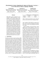
3.3 Representation of n-gram language models
An n-gram model can be efficiently represented in a de-
terministic WFA, through the use of failure transitions
(Allauzen et al., 2003). Every string accepted by such an
automaton has a single path through the automaton, and

the weight of the string is the sum of the weights of the
transitions in that path. In such a representation, every
state in the automaton represents an n-gram history h,
e.g. w
i−2
w
i−1
, and there are transitions leaving the state
for every word w
i
such that the feature hw
i
has a weight.
There is also a failure transition leaving the state, labeled
with some reserved symbol φ, which can only be tra-
versed if the next symbol in the input does not match any
transition leaving the state. This failure transition points
to the backoff state h

, i.e. the n-gram history h minus
its initial word. Figure 2 shows how a trigram model can
be represented in such an automaton. See Allauzen et al.
(2003) for more details.
Note that in such a deterministic representation, the
entire weight of all features associated with the word
w
i
following history h must be assigned to the transi-
tion labeled with w
i

leaving the state h in the automa-
ton. For example, if h = w
i−2
w
i−1
, then the trigram
w
i−2
w
i−1
w
i
is a feature, as is the bigram w
i−1
w
i
and
the unigram w
i
. In this case, the weight on the transi-
tion w
i
leaving state h must be the sum of the trigram,
bigram and unigram feature weights. If only the trigram
feature weight were assigned to the transition, neither the
unigram nor the bigram feature contribution would be in-
cluded in the path weight. In order to ensure that the cor-
rect weights are assigned to each string, every transition
encoding an order k n-gram must carry the sum of the
weights for all n-gram features of orders ≤ k. To ensure

that every string in Σ
∗
receives the correct weight, for
any n-gram hw represented explicitly in the automaton,
h

w must also be represented explicitly in the automaton,
even if its weight is 0.
3.4 The perceptron algorithm
The perceptron algorithm is incremental, meaning that
the language model D is built one training example at
a time, during several passes over the training set. Ini-
tially, we build D to accept all strings in Σ
∗
with weight
0. For the perceptron experiments, we chose the param-
eter α
0
to be a fixed constant, chosen by optimization on
the held-out set. The loop in the algorithm in figure 1 is
implemented as:
For t = 1 . . . T, i = 1 . . . N :
• Calculate z
i
= argmax
y∈GEN(x)
Φ(x, y) · ¯α
= BestPath(α
0
L

i
◦ D)
• If z
i
= MinErr(L
i
, r
i
), then update the feature
weights as in figure 1 (modulo the sign, because of
the use of costs), and modify D so as to assign the
correct weight to all strings.
In addition, averaged parameters need to be stored
(see section 2.2). These parameters will replace the un-
averaged parameters in D once training is completed.
Note that the only n-gram features to be included in
D at the end of the training process are those that oc-
cur in either a best scoring path z
i
or a minimum error
path y
i
at some point during training. Thus the percep-
tron algorithm is in effect doing feature selection as a
by-product of training. Given N training examples, and
T passes over the training set, O(NT ) n-grams will have
non-zero weight after training. Experiments in Roark et
al. (2004) suggest that the perceptron reaches optimal
performance after a small number of training iterations,
for example T = 1 or T = 2. Thus O(NT) can be very

small compared to the full number of n-grams seen in
all training lattices. In our experiments, the perceptron
method chose around 1.4 million n-grams with non-zero
weight. This compares to 43.65 million possible n-grams
seen in the training data.
This is a key contrast with conditional random fields,
which optimize the parameters of a fixed feature set. Fea-
ture selection can be critical in our domain, as training
and applying a discriminative language model over all
n-grams seen in the training data (in either correct or in-
correct transcriptions) may be computationally very de-
manding. One training scenario that we will consider
will be using the output of the perceptron algorithm (the
averaged parameters) to provide the feature set and the
initial feature weights for use in the CRF algorithm. This
leads to a model which is reasonably sparse, but has the
benefit of CRF training, which as we will see gives gains
in performance.
3.5 Conditional Random Fields
The CRF methods that we use assume a fixed definition
of the n-gram features Φ
i
for i = 1 . . . d in the model.
In the experimental section we will describe a number of
ways of defining the feature set. The optimization meth-
ods we use begin at some initial setting for ¯α, and then
search for the parameters ¯α
∗
which maximize LL
R

(¯α)
as defined in Eq. 3.
The optimization method requires calculation of
LL
R
(¯α) and the gradient of LL
R
(¯α) for a series of val-
ues for ¯α. The first step in calculating these quantities is
to take the parameter values ¯α, and to construct an ac-
ceptor D which accepts all strings in Σ
∗
, such that
w
D
[π] =
d

j=1
Φ
j
(x, l[π])α
j
For each training lattice L
i
, we then construct a new lat-
tice L

i
= Norm(α

0
L
i
◦ D). The lattice L

i
represents
(in the log domain) the distribution p
¯α
(y|x
i
) over strings
y ∈ GEN(x
i
). The value of log p
¯α
(y
i
|x
i
) for any i can
be computed by simply taking the path weight of π such
that l[π] = y
i
in the new lattice L

i
. Hence computation
of LL
R

(¯α) in Eq. 3 is straightforward.
Calculating the n-gram feature gradients for the CRF
optimization is also relatively simple, once L

i
has been
constructed. From the derivative in Eq. 4, for each i =
1 . . . N, j = 1 . . . d the quantity
Φ
j
(x
i
, y
i
) −

y∈GEN(x
i
)
p
¯α
(y|x
i
)Φ
j
(x
i
, y) (8)
must be computed. The first term is simply the num-
ber of times the j’th n-gram feature is seen in y

i
. The
second term is the expected number of times that the
j’th n-gram is seen in the acceptor L

i
. If the j’th
n-gram is w
1
. . . w
n
, then this can be computed as
ExpCount(L

i
, w
1
. . . w
n
). The GRM library, which
was presented in Allauzen et al. (2003), has a direct im-
plementation of the function ExpCount, which simul-
taneously calculates the expected value of all n-grams of
order less than or equal to a given n in a lattice L.
The one non-ngram feature weight that is being esti-
mated is the weight α
0
given to the baseline ASR nega-
tive log probability. Calculation of the gradient of LL
R

with respect to this parameter again requires calculation
of the term in Eq. 8 for j = 0 and i = 1 . . . N. Com-
putation of

y∈GEN(x
i
)
p
¯α
(y|x
i
)Φ
0
(x
i
, y) turns out to
be not as straightforward as calculating n-gram expec-
tations. To do so, we rely upon the fact that Φ
0
(x
i
, y),
the negative log probability of the path, decomposes to
the sum of negative log probabilities of each transition
in the path. We index each transition in the lattice L
i
,
and store its negative log probability under the baseline
model. We can then calculate the required gradient from
L


i
, by calculating the expected value in L

i
of each in-
dexed transition in L
i
.
We found that an approximation to the gradient of
α
0
, however, performed nearly identically to this exact
gradient, while requiring substantially less computation.
Let w
n
1
be a string of n words, labeling a path in word-
lattice L

i
. For brevity, let P
i
(w
n
1
) = p
¯α
(w
n

1
|x
i
) be the
conditional probability under the current model, and let
Q
i
(w
n
1
) be the probability of w
n
1
in the normalized base-
line ASR lattice Norm(L
i
). Let L
i
be the set of strings
in the language defined by L
i
. Then we wish to compute
E
i
for i = 1 . . . N , where
E
i
=

w

n
1
∈L
i
P
i
(w
n
1
) log Q
i
(w
n
1
)
=

w
n
1
∈L
i

k=1 n
P
i
(w
n
1
) log Q

i
(w
k
|w
k−1
1
) (9)
The approximation is to make the following Markov
assumption:
E
i
≈

w
n
1
∈L
i

k=1 n
P
i
(w
n
1
) log Q
i
(w
k
|w

k−1
k−2
)
=

xyz∈S
i
ExpCount(L

i
, xyz) log Q
i
(z|xy)(10)
where S
i
is the set of all trigrams seen in L
i
. The term
log Q
i
(z|xy) can be calculated once before training for
every lattice in the training set; the ExpCount term is
calculated as before using the GRM library. We have
found this approximation to be effective in practice, and
it was used for the trials reported below.
When the gradients and conditional likelihoods are
collected from all of the utterances in the training set, the
contributions from the regularizer are combined to give
an overall gradient and objective function value. These
values are provided to the parameter estimation routine,

which then returns the parameters for use in the next it-
eration. The accumulation of gradients for the feature set
is the most time consuming part of the approach, but this
is parallelizable, so that the computation can be divided
among many processors.
4 Empirical Results
We present empirical results on the Rich Transcription
2002 evaluation test set (rt02), which we used as our de-
velopment set, as well as on the Rich Transcription 2003
Spring evaluation CTS test set (rt03). The rt02 set con-
sists of 6081 sentences (63804 words) and has three sub-
sets: Switchboard 1, Switchboard 2, Switchboard Cel-
lular. The rt03 set consists of 9050 sentences (76083
words) and has two subsets: Switchboard and Fisher.
We used the same training set as that used in Roark
et al. (2004). The training set consists of 276726 tran-
scribed utterances (3047805 words), with an additional
20854 utterances (249774 words) as held out data. For
0 500 1000
37
37.5
38
38.5
39
39.5
40
Iterations over training
Word error rate
Baseline recognizer
Perceptron, Feat=PL, Lattice

Perceptron, Feat=PN, N=1000
CRF, σ = ∞, Feat=PL, Lattice
CRF, σ = 0.5, Feat=PL, Lattice
CRF, σ = 0.5, Feat=PN, N=1000
Figure 3: Word error rate on the rt02 eval set versus training
iterations for CRF trials, contrasted with baseline recognizer
performance and perceptron performance. Points are at every
20 iterations. Each point (x,y) is the WER at the iteration with
the best objective function value in the interval (x-20,x].
each utterance, a weighted word-lattice was produced,
representing alternative transcriptions, from the ASR
system. From each word-lattice, the oracle best path
was extracted, which gives the best word-error rate from
among all of the hypotheses in the lattice. The oracle
word-error rate for the training set lattices was 12.2%.
We alsoperformed trials with 1000-best lists for the same
training set, rather than lattices. The oracle score for the
1000-best lists was 16.7%.
To produce the word-lattices, each training utterance
was processed by the baseline ASR system. However,
these same utterances are what the acoustic and language
models are built from, which leads to better performance
on the training utterances than can be expected when the
ASR system processes unseen utterances. To somewhat
control for this, the training set was partitioned into 28
sets, and baseline Katz backoff trigram models were built
for each set by including only transcripts from the other
27 sets. Since language models are generally far more
prone to overtrain than standard acoustic models, this
goes a long way toward making the training conditions

similar to testing conditions.
There are three baselines against which we are com-
paring. The first is the ASR baseline, with no reweight-
ing from a discriminatively trained n-gram model. The
other two baselines are with perceptron-trained n-gram
model re-weighting, and were reported in Roark et al.
(2004). The first of these is for a pruned-lattice trained
trigram model, which showed a reduction in word er-
ror rate (WER) of 1.3%, from 39.2% to 37.9% on rt02.
The second is for a 1000-best list trained trigram model,
which performed only marginally worse than the lattice-
trained perceptron, at 38.0% on rt02.
4.1 Perceptron feature set
We use the perceptron-trained models as the starting
point for our CRF algorithm: the feature set given to
the CRF algorithm is the feature set selected by the per-
ceptron algorithm; the feature weights are initialized to
those of the averaged perceptron. Figure 3 shows the
performance of our three baselines versus three trials of
0 500 1000 1500 2000 2500
37
37.5
38
38.5
39
39.5
40
Iterations over training
Word error rate
Baseline recognizer

Perceptron, Feat=PL, Lattice
CRF, σ = 0.5, Feat=PL, Lattice
CRF, σ = 0.5, Feat=E, θ=0.01
CRF, σ = 0.5, Feat=E, θ=0.9
Figure 4: Word error rate on the rt02 eval set versus training
iterations for CRF trials, contrasted with baseline recognizer
performance and perceptron performance. Points are at every
20 iterations. Each point (x,y) is the WER at the iteration with
the best objective function value in the interval (x-20,x].
the CRF algorithm. In the first two trials, the training
set consists of the pruned lattices, and the feature set
is from the perceptron algorithm trained on pruned lat-
tices. There were 1.4 million features in this feature set.
The first trial set the regularizer constant σ = ∞, so that
the algorithm was optimizing raw conditional likelihood.
The second trial is with the regularizer constant σ = 0.5,
which we found empirically to be a good parameteriza-
tion on the held-out set. As can be seen from these re-
sults, regularization is critical.
The third trial in this set uses the feature set from the
perceptron algorithm trained on 1000-best lists, and uses
CRF optimization on these on these same 1000-best lists.
There were 0.9 million features in this feature set. For
this trial, we also used σ = 0.5. As with the percep-
tron baselines, the n-best trial performs nearly identically
with the pruned lattices, here also resulting in 37.4%
WER. This may be useful for techniques that would be
more expensive to extend to lattices versus n-best lists
(e.g. models with unbounded dependencies).
These trials demonstrate that the CRF algorithm can

do a better job of estimating feature weights than the per-
ceptron algorithm for the same feature set. As mentioned
in the earlier section, feature selection is a by-product of
the perceptron algorithm, but the CRF algorithm is given
a set of features. The next two trials looked at selecting
feature sets other than those provided by the perceptron
algorithm.
4.2 Other feature sets
In order for the feature weights to be non-zero in this ap-
proach, they must be observed in the training set. The
number of unigram, bigram and trigram features with
non-zero observations in the training set lattices is 43.65
million, or roughly 30 times the size of the perceptron
feature set. Many of these features occur only rarely
with very low conditional probabilities, and hence cannot
meaningfully impact system performance. We pruned
this feature set to include all unigrams and bigrams, but
only those trigrams with an expected count of greater
than 0.01 in the training set. That is, to be included, a
Trial Iter rt02 rt03
ASR Baseline - 39.2 38.2
Perceptron, Lattice - 37.9 36.9
Perceptron, N-best - 38.0 37.2
CRF, Lattice, Percep Feats (1.4M) 769 37.4 36.5
CRF, N-best, Percep Feats (0.9M) 946 37.4 36.6
CRF, Lattice, θ = 0.01 (12M) 2714 37.6 36.5
CRF, Lattice, θ = 0.9 (1.5M) 1679 37.5 36.6
Table 1: Word-error rate results at convergence iteration for
various trials, on both Switchboard 2002 test set (rt02), which
was used as the dev set, and Switchboard 2003 test set (rt03).

trigram must occur in a set of paths, the sum of the con-
ditional probabilities of which must be greater than our
threshold θ = 0.01. This threshold resulted in a feature
set of roughly 12 million features, nearly 10 times the
size of the perceptron feature set. For better comparabil-
ity with that feature set, we set our thresholds higher, so
that trigrams were pruned if their expected count fell be-
low θ = 0.9, and bigrams were pruned if their expected
count fell below θ = 0.1. We were concerned that this
may leave out some of the features on the oracle paths, so
we added back in all bigram and trigram features that oc-
curred on oracle paths, giving a feature set of 1.5 million
features, roughly the same size as the perceptron feature
set.
Figure 4 shows the results for three CRF trials versus
our ASR baseline and the perceptron algorithm baseline
trained on lattices. First, the result using the perceptron
feature set provides us with a WER of 37.4%, as pre-
viously shown. The WER at convergence for the big
feature set (12 million features) is 37.6%; the WER at
convergence for the smaller feature set (1.5 million fea-
tures) is 37.5%. While both of these other feature sets
converge to performance close to that using the percep-
tron features, the number of iterations over the training
data that are required to reach that level of performance
are many more than for the perceptron-initialized feature
set.
Table 1 shows the word-error rate at the convergence
iteration for the various trials, on both rt02 and rt03. All
of the CRF trials are significantly better than the percep-

tron performance, using the Matched Pair Sentence Seg-
ment test for WER included with SCTK (NIST, 2000).
On rt02, the N-best and perceptron initialized CRF trials
were were significantly better than the lattice perceptron
at p < 0.001; the other two CRF trials were significantly
better than the lattice perceptron at p < 0.01. On rt03,
the N-best CRF trial was significantly better than the lat-
tice perceptron at p < 0.002; the other three CRF tri-
als were significantly better than the lattice perceptron at
p < 0.001.
Finally, we measured the time of a single iteration over
the training data on a single machine for the perceptron
algorithm, the CRF algorithm using the approximation to
the gradient of α
0
, and the CRF algorithm using an exact
gradient of α
0
. Table 2 shows these times in hours. Be-
cause of the frequent update of the weights in the model,
the perceptron algorithm is more expensive than the CRF
algorithm for a single iteration. Further, the CRF algo-
rithm is parallelizable, so that most of the work of an
CRF
Features Percep approx exact
Lattice, Percep Feats (1.4M) 7.10 1.69 3.61
N-best, Percep Feats (0.9M) 3.40 0.96 1.40
Lattice, θ = 0.01 (12M) - 2.24 4.75
Table 2: Time (in hours) for one iteration on a single Intel
Xeon 2.4Ghz processor with 4GB RAM.

iteration can be shared among multiple processors. Our
most common training setup for the CRF algorithm was
parallelized between 20 processors, using the approxi-
mation to the gradient. In that setup, using the 1.4M fea-
ture set, one iteration of the perceptron algorithm took
the same amount of real time as approximately 80 itera-
tions of CRF.
5 Conclusion
We have contrasted two approaches to discriminative
language model estimation on a difficult large vocabu-
lary task, showing that they can indeed scale effectively
to handle this size of a problem. Both algorithms have
their benefits. The perceptron algorithm selects a rela-
tively small subset of the total feature set, and requires
just a couple of passes over the training data. The CRF
algorithm does a better job of parameter estimation for
the same feature set, and is parallelizable, so that each
pass over the training set can require just a fraction of
the real time of the perceptron algorithm.
The best scenario from among those that we investi-
gated was a combination of both approaches, with the
output of the perceptron algorithm taken as the starting
point for CRF estimation.
As a final point, note that the methods we describe do
not replace an existing language model, but rather com-
plement it. The existing language model has the benefit
that it can be trained on a large amount of text that does
not have speech transcriptions. It has the disadvantage
of not being a discriminative model. The new language
model is trained on the speech transcriptions, meaning

that it has less training data, but that it has the advan-
tage of discriminative training – and in particular, the ad-
vantage of being able to learn negative evidence in the
form of negative weights on n-grams which are rarely
or never seen in natural language text (e.g., “the of”),
but are produced too frequently by the recognizer. The
methods we describe combines the two language models,
allowing them to complement each other.
References
Cyril Allauzen, Mehryar Mohri, and Brian Roark. 2003. Generalized
algorithms for constructing language models. In Proceedings of the
41st Annual Meeting of the Association for Computational Linguis-
tics, pages 40–47.
Satish Balay, William D. Gropp, Lois Curfman McInnes, and Barry F.
Smith. 2002. Petsc users manual. Technical Report ANL-95/11-
Revision 2.1.2, Argonne National Laboratory.
Satanjeev Banerjee, Jack Mostow, Joseph Beck, and Wilson Tam.
2003. Improving language models by learning from speech recog-
nition errors in a reading tutor that listens. In Proceedings of the
Second International Conference on Applied Artificial Intelligence,
Fort Panhala, Kolhapur, India.
Steven J. Benson and Jorge J. Mor
´
e. 2002. A limited memory vari-
able metric method for bound constrained minimization. Preprint
ANL/ACSP909-0901, Argonne National Laboratory.
Steven J. Benson, Lois Curfman McInnes, Jorge J. Mor
´
e, and Jason
Sarich. 2002. Tao users manual. Technical Report ANL/MCS-TM-

242-Revision 1.4, Argonne National Laboratory.
Zheng Chen, Kai-Fu Lee, and Ming Jing Li. 2000. Discriminative
training on language model. In Proceedings of the Sixth Interna-
tional Conference on Spoken Language Processing (ICSLP), Bei-
jing, China.
Michael Collins. 2002. Discriminative training methods for hidden
markov models: Theory and experiments with perceptron algo-
rithms. In Proceedings of the Conference on Empirical Methods
in Natural Language Processing (EMNLP), pages 1–8.
Michael Collins. 2004. Parameter estimation for statistical parsing
models: Theory and practice of distribution-free methods. In Harry
Bunt, John Carroll, and Giorgio Satta, editors, New Developments
in Parsing Technology. Kluwer.
Yoav Freund and Robert Schapire. 1999. Large margin classification
using the perceptron algorithm. Machine Learning, 3(37):277–296.
Frederick Jelinek. 1995. Acoustic sensitive language modeling. Tech-
nical report, Center for Language and Speech Processing, Johns
Hopkins University, Baltimore, MD.
Mark Johnson, Stuart Geman, Steven Canon, Zhiyi Chi, and Stefan
Riezler. 1999. Estimators for stochastic “unification-based” gram-
mars. In Proceedings of the 37th Annual Meeting of the Association
for Computational Linguistics, pages 535–541.
Sanjeev Khudanpur and Jun Wu. 2000. Maximum entropy techniques
for exploiting syntactic, semantic and collocational dependencies in
language modeling. Computer Speech and Language, 14(4):355–
372.
Hong-Kwang Jeff Kuo, Eric Fosler-Lussier, Hui Jiang, and Chin-
Hui Lee. 2002. Discriminative training of language models for
speech recognition. In Proceedings of the International Conference
on Acoustics, Speech, and Signal Processing (ICASSP), Orlando,

Florida.
John Lafferty, Andrew McCallum, and Fernando Pereira. 2001. Con-
ditional random fields: Probabilistic models for segmenting and
labeling sequence data. In Proc. ICML, pages 282–289, Williams
College, Williamstown, MA, USA.
Robert Malouf. 2002. A comparison of algorithms for maximum en-
tropy parameter estimation. In Proc. CoNLL, pages 49–55.
Andrew McCallum and Wei Li. 2003. Early results for named entity
recognition with conditional random fields, feature induction and
web-enhanced lexicons. In Proc. CoNLL.
Mehryar Mohri, Fernando C. N. Pereira, and Michael Riley. 2002.
Weighted finite-state transducers in speech recognition. Computer
Speech and Language, 16(1):69–88.
NIST. 2000. Speech recognition scoring toolkit (sctk) version 1.2c.
Available at />David Pinto, Andrew McCallum, Xing Wei, and W. Bruce Croft. 2003.
Table extraction using conditional random fields. In Proc. ACM SI-
GIR.
Adwait Ratnaparkhi, Salim Roukos, and R. Todd Ward. 1994. A max-
imum entropy model for parsing. In Proceedings of the Interna-
tional Conference on Spoken Language Processing (ICSLP), pages
803–806.
Brian Roark, Murat Saraclar, and Michael Collins. 2004. Corrective
language modeling for large vocabulary ASR with the perceptron al-
gorithm. In Proceedings of the International Conference on Acous-
tics, Speech, and Signal Processing (ICASSP), pages 749–752.
Fei Sha and Fernando Pereira. 2003. Shallow parsing with conditional
random fields. In Proc. HLT-NAACL, Edmonton, Canada.
A. Stolcke and M. Weintraub. 1998. Discriminitive language model-
ing. In Proceedings of the 9th Hub-5 Conversational Speech Recog-
nition Workshop.

A. Stolcke, H. Bratt, J. Butzberger, H. Franco, V. R. Rao Gadde,
M. Plauche, C. Richey, E. Shriberg, K. Sonmez, F. Weng, and
J. Zheng. 2000. The SRI March 2000 Hub-5 conversational speech
transcription system. In Proceedings of the NIST Speech Transcrip-
tion Workshop.
Hanna Wallach. 2002. Efficient training of conditional random fields.
Master’s thesis, University of Edinburgh.
P.C. Woodland and D. Povey. 2000. Large scale discriminative training
for speech recognition. In Proc. ISCA ITRW ASR2000, pages 7–16.