Báo cáo khoa học: "Alternative Approaches for Generating Bodies of Grammar Rules" docx
Bạn đang xem bản rút gọn của tài liệu. Xem và tải ngay bản đầy đủ của tài liệu tại đây (96.74 KB, 8 trang )
Alternative Approaches for Generating Bodies of Grammar Rules
Gabriel Infante-Lopez and Maarten de Rijke
Informatics Institute, University of Amsterdam
{infante,mdr}@science.uva.nl
Abstract
We compare two approaches for describing and gen-
erating bodies of rules used for natural language
parsing. In today’s parsers rule bodies do not ex-
ist a priori but are generated on the fly, usually with
methods based on n-grams, which are one particu-
lar way of inducing probabilistic regular languages.
We compare two approaches for inducing such lan-
guages. One is based on n-grams, the other on min-
imization of the Kullback-Leibler divergence. The
inferred regular languages are used for generating
bodies of rules inside a parsing procedure. We com-
pare the two approaches along two dimensions: the
quality of the probabilistic regular language they
produce, and the performance of the parser they
were used to build. The second approach outper-
forms the first one along both dimensions.
1 Introduction
N-grams have had a big impact on the state of the
art in natural language parsing. They are central
to many parsing models (Charniak, 1997; Collins,
1997, 2000; Eisner, 1996), and despite their sim-
plicity n-gram models have been very successful.
Modeling with n-grams is an induction task (Gold,
1967). Given a sample set of strings, the task is to
guess the grammar that produced that sample. Usu-
ally, the grammar is not be chosen from an arbitrary
set of possible grammars, but from a given class.
Hence, grammar induction consists of two parts:
choosing the class of languages amongst which to
search and designing the procedure for performing
the search. By using n-grams for grammar induc-
tion one addresses the two parts in one go. In par-
ticular, the use of n-grams implies that the solu-
tion will be searched for in the class of probabilis-
tic regular languages, since n-grams induce prob-
abilistic automata and, consequently, probabilistic
regular languages. However, the class of probabilis-
tic regular languages induced using n-grams is a
proper subclass of the class of all probabilistic reg-
ular languages; n-grams are incapable of capturing
long-distance relations between words. At the tech-
nical level the restricted nature of n-grams is wit-
nessed by the special structure of the automata in-
duced from them, as we will see in Section 4.2.
N-grams are not the only way to induce regular
languages, and not the most powerful way to do so.
There is a variety of general methods capable of in-
ducing all regular languages (Denis, 2001; Carrasco
and Oncina, 1994; Thollard et al., 2000). What is
their relevance for natural language parsing? Re-
call that regular languages are used for describing
the bodies of rules in a grammar. Consequently, the
quality and expressive power of the resulting gram-
mar is tied to the quality and expressive power of the
regular languages used to describe them. And the
quality and expressive power of the latter, in turn,
are influenced directly by the method used to induce
them. These observations give rise to a natural ques-
tion: can we gain anything in parsing from using
general methods for inducing regular languages in-
stead of methods based on n-grams? Specifically,
can we describe the bodies of grammatical rules
more accurately and more concisely by using gen-
eral methods for inducing regular languages?
In the context of natural language parsing we
present an empirical comparison between algo-
rithms for inducing regular languages using n-
grams on the one hand, and more general algorithms
for learning the general class of regular language on
the other hand. We proceed as follows. We gen-
erate our training data from the Wall Street Journal
Section of the Penn Tree Bank (PTB), by transform-
ing it to projective dependency structures, following
(Collins, 1996), and extracting rules from the result.
These rules are used as training material for the rule
induction algorithms we consider. The automata
produced this way are then used to build grammars
which, in turn, are used for parsing.
We are interested in two different aspects of the
use of probabilistic regular languages for natural
language parsing: the quality of the induced au-
tomata and the performance of the resulting parsers.
For evaluation purposes, we use two different met-
rics: perplexity for the first aspect and percentage
of correct attachments for the second. The main re-
sults of the paper are that, measured in terms of per-
plexity, the automata induced by algorithms other
than n-grams describe the rule bodies better than
automata induced using n-gram-based algorithms,
and that, moreover, the gain in automata quality
is reflected by an improvement in parsing perfor-
mance. We also find that the parsing performance
of both methods (n-grams vs. general automata) can
be substantially improved by splitting the training
material into POS categories. As a side product,
we find empirical evidence to suggest that the effec-
tiveness of rule lexicalization techniques (Collins,
1997; Sima’an, 2000) and parent annotation tech-
niques (Klein and Manning, 2003) is due to the fact
that both lead to a reduction in perplexity in the au-
tomata induced from training corpora.
Section 2 surveys our experiments, and later sec-
tions provide details of the various aspects. Sec-
tion 3 offers details on our grammatical frame-
work, PCW-grammars, on transforming automata
to PCW-grammars, and on parsing with PCW-
grammars. Section 4 explains the starting point of
this process: learning automata, and Section 5 re-
ports on parsing experiments. We discuss related
work in Section 6 and conclude in Section 7.
2 Overview
We want to build grammars using different algo-
rithms for inducing their rules. Our main question
is aimed at understanding how different algorithms
for inducing regular languages impact the parsing
performance with those grammars. A second issue
that we want to explore is how the grammars per-
form when the quality of the training material is im-
proved, that is, when the training material is sep-
arated into part of speech (POS) categories before
the regular language learning algorithms are run.
We first transform the PTB into projective depen-
dencies structures following (Collins, 1996). From
the resulting tree bank we delete all lexical informa-
tion except POS tags. Every POS in a tree belonging
to the tree-bank has associated to it two different,
possibly empty, sequences of right and left depen-
dents, respectively. We extract all these sequences
for all trees, producing two different sets containing
right and left sequences of dependents respectively.
These two sets form the training material used for
building four different grammars. The four gram-
mars differ along two dimensions: the number of
automata used for building them and the algorithm
used for inducing the automata. As to the latter di-
mension, in Section 4 we use two algorithms: the
Minimum Discriminative Information (MDI) algo-
rithm, and a bigram-based algorithm. As to the for-
mer dimension, two of the grammars are built us-
ing only two different automata, each of which is
built using the two sample set generated from the
PTB. The other two grammars were built using two
automata per POS, exploiting a split of the train-
ing samples into multiple samples, two samples per
POS, to be precise, each containing only those sam-
ples where the POS appeared as the head.
The grammars built from the induced automata
are so-called PCW-grammars (see Section 3), a for-
malism based on probabilistic context free gram-
mars (PCFGs); as we will see in Section 3, inferring
them from automata is almost immediate.
3 Grammatical Framework
We briefly detail the grammars we work with
(PCW-grammars), how automata give rise to these
grammars, and how we parse using them.
3.1 PCW-Grammars
We need a grammatical framework that models
rule bodies as instances of a regular language and
that allows us to transform automata to gram-
mars as directly as possible. We decided to em-
bed them in the general grammatical framework of
CW-grammars (Infante-Lopez and de Rijke, 2003):
based on PCFGs, they have a clear and well-
understood mathematical background and we do not
need to implement ad-hoc parsing algorithms.
A probabilistic constrained W-grammar (PCW-
grammar) consists of two different sets of PCF-like
rules called pseudo-rules and meta-rules respec-
tively and three pairwise disjoint sets of symbols:
variables, non-terminals and terminals. Pseudo-
rules and meta-rules provide mechanisms for build-
ing ‘real’ rewrite rules. We use α
w
=⇒ β to indicate
that α should be rewritten as β. In the case of PCW-
grammars, rewrite rules are built by first selecting a
pseudo-rule, and then using meta-rules for instanti-
ating all the variables in the body of the pseudo-rule.
To illustrate these concepts, we provide an exam-
ple. Let W = (V, N T, T, S,
m
−→,
s
−→) be a CW-
grammar such that the set of variable, non-terminals
meta-rules
pseudo-rules
Adj
m
−→
0.5
AdjAdj S
s
−→
1
Adj Noun
Adj
m
−→
0.5
Adj Adj
s
−→
0.1
big
Noun
s
−→
1
ball
.
.
.
and terminals are defined as follows: V = {
Adj },
NT = {S, Adj , Noun}, T = {ball , big, fat,
red, green, . . .}. As usual, the numbers attached
to the arrows indicate the probabilities of the rules.
The rules defined by W have the following shape:
S
w
=⇒ Adj
∗
Noun. Suppose now that we want to
build the rule S
w
=⇒ Adj Adj Noun. We take the
pseudo-rule S
s
−→
1
Adj Noun and instantiate the
variable Adj with Adj Adj to get the desired rule.
The probability for it is 1 × 0.5 × 0.5, that is, the
probability of the derivation for Adj Adj times the
probability of the pseudo-rule used. Trees for this
particular grammar are flat, with a main node S and
all the adjectives in it as daughters. An example
derivation is given in Figure 1(a).
3.2 From Automata to Grammars
Now that we have introduced PCW-grammars, we
describe how we build them from the automata
that we are going to induce in Section 4. Since
we will induce two families of automata (“Many-
Automata” where we use two automata per POS,
and “One-Automaton” where we use only two au-
tomata to fit every POS), we need to describe two
automata-to-grammar transformations.
Let’s start with the case where we build two au-
tomata per POS. Let w be a POS in the PTB; let A
w
L
and A
w
R
be the two automata associated to it. Let G
w
L
and G
w
R
be the PCFGs equivalent to A
w
L
and A
w
R
, re-
spectively, following (Abney et al., 1999), and let
S
w
L
and S
w
R
be the starting symbols of G
w
L
and G
w
R
,
respectively. We build our final grammar G with
starting symbol S, by defining its meta-rules as the
disjoint union of all rules in G
w
L
and G
w
R
(for all POS
w), its set of pseudo-rules as the union of the sets
{W
s
−→
1
S
w
L
wS
w
R
and S
s
−→
1
S
w
L
wS
w
R
}, where
W is a unique new variable symbol associated to w.
When we use two automata for all parts of
speech, the grammar is defined as follows. Let A
L
and A
R
be the two automata learned. Let G
L
and
G
R
be the PCFGs equivalent to A
L
and A
R
, and let
S
L
and S
R
be the starting symbols of G
L
and G
R
,
respectively. Fix a POS w in the PTB. Since the au-
tomata are deterministic, there exist states S
w
L
and
S
w
R
that are reachable from S
L
and S
R
, respectively,
by following the arc labeled with w. Define a gram-
mar as in the previous case. Its starting symbol is S,
its set of meta-rules is the disjoint union of all rules
in G
w
L
and G
w
R
(for all POS w), its set of pseudo-
rules is {W
s
−→
1
S
w
L
wS
w
R
, S
s
−→
1
S
w
L
wS
w
R
:
w is a POS in the PTB and W is a unique new vari-
able symbol associated to w}.
3.3 Parsing PCW-Grammars
Parsing PCW-grammars requires two steps: a
generation-rule step followed by a tree-building
step. We now explain how these two steps can be
carried out in one go. Parsing with PCW-grammars
can be viewed as parsing with PCF grammars. The
main difference is that in PCW-parsing derivations
for variables remain hidden in the final tree. To clar-
ify this, consider the trees depicted in Figure 1; the
tree in part (a) is the CW-tree corresponding to the
word red big green ball, and the tree in part (b) is
the same tree but now the instantiations of the meta-
rules that were used have been made visible.
S
Adj
red
Adj
big
Adj
green
Noun
ball
S
Adj
1
Adj
1
Adj
1
Adj
red
Adj
big
Adj
green
Noun
ball
(a) (b)
Figure 1: (a) A tree generated by W . (b) The same
tree with meta-rule derivations made visible.
To adapt a PCFG to parse CW-grammars, we
need to define a PCF grammar for a given PCW-
grammar by adding the two sets of rules while mak-
ing sure that all meta-rules have been marked some-
how. In Figure 1(b) the head symbols of meta-rules
have been marked with the superscript 1. After pars-
ing the sentence with the PCF parser, all marked
rules should be collapsed as shown in part (a).
4 Building Automata
The four grammars we intend to induce are com-
pletely defined once the underlying automata have
been built. We now explain how we build those au-
tomata from the training material. We start by de-
tailing how the material is generated.
4.1 Building the Sample Sets
We transform the PTB, sections 2–22, to depen-
dency structures, as suggested by (Collins, 1999).
All sentences containing CC tags are filtered out,
following (Eisner, 1996). We also eliminate all
word information, leaving only POS tags. For each
resulting dependency tree we extract a sample set of
right and left sequences of dependents as shown in
Figure 2. From the tree we generate a sample set
with all right sequences of dependents {, , }, and
another with all left sequences {, , red big green}.
The sample set used for automata induction is the
union of all individual tree sample sets.
4.2 Learning Probabilistic Automata
Probabilistic deterministic finite state automata
(PDFA) inference is the problem of inducing a
stochastic regular grammar from a sample set of
strings belonging to an unknown regular language.
The most direct approach for solving the task is by
S
JJ
jj
red
JJ
jj
big
JJ
jj
green
nn
ball
ballgreenbigr ed
(a) (b)
jj jj nn
left right left right left right
red big green
(c)
Figure 2: (a), (b) Dependency representations of
Figure 1. (c) Sample instances extracted from this
tree.
using n-grams. The n-gram induction algorithm
adds a state to the resulting automaton for each se-
quence of symbols of length n it has seen in the
training material; it also adds an arc between states
aβ and βb labeled b, if the sequence aβb appears
in the training set. The probability assigned to the
arc (aβ, βb) is proportional to the number of times
the sequence aβb appears in the training set. For the
remainder, we take n-grams to be bigrams.
There are other approaches to inducing regular
grammars besides ones based on n -grams. The first
algorithm to learn PDFAs was ALERGIA (Carrasco
and Oncina, 1994); it learns cyclic automata with
the so-called state-merging method. The Minimum
Discrimination Information (MDI) algorithm (Thol-
lard et al., 2000) improves over ALERGIA and uses
Kullback-Leibler divergence for deciding when to
merge states. We opted for the MDI algorithm as
an alternative to n-gram based induction algorithms,
mainly because their working principles are rad-
ically different from the n-gram-based algorithm.
The MDI algorithm first builds an automaton that
only accepts the strings in the sample set by merg-
ing common prefixes, thus producing a tree-shaped
automaton in which each transition has a probability
proportional to the number of times it is used while
generating the positive sample.
The MDI algorithm traverses the lattice of all
possible partitions for this general automaton, at-
tempting to merge states that satisfy a trade-off that
can be specified by the user. Specifically, assume
that A
1
is a temporary solution of the algorithm
and that A
2
is a tentative new solution derived from
A
1
. ∆(A
1
, A
2
) = D(A
0
||A
2
) − D(A
0
||A
1
) de-
notes the divergence increment while going from
A
1
to A
2
, where D(A
0
||A
i
) is the Kullback-Leibler
divergence or relative entropy between the two
distributions generated by the corresponding au-
tomata (Cover and Thomas, 1991). The new solu-
tion A
2
is compatible with the training data if the
divergence increment relative to the size reduction,
that is, the reduction of the number of states, is small
enough. Formally, let alpha denote a compatibil-
ity threshold; then the compatibility is satisfied if
∆(A
1
,A
2
)
|A
1
|−|A
2
|
< alph a. For this learning algorithm,
alpha is the unique parameter; we tuned it to get
better quality automata.
4.3 Optimizing Automata
We use three measures to evaluate the quality of
a probabilistic automaton (and set the value of
alpha optimally). The first, called test sample
perplexity (PP), is based on the per symbol log-
likelihood of strings x belonging to a test sam-
ple according to the distribution defined by the au-
tomaton. Formally, LL = −
1
|S|
x∈S
log (P (x)),
where P (x) is the probability assigned to the string
x by the automata. The perplexity PP is defined as
P P = 2
LL
. The minimal perplexity P P = 1 is
reached when the next symbol is always predicted
with probability 1 from the current state, while
P P = |Σ| corresponds to uniformly guessing from
an alphabet of size |Σ|.
The second measure we used to evaluate the qual-
ity of an automaton is the number of missed samples
(MS). A missed sample is a string in the test sam-
ple that the automaton failed to accept. One such
instance suffices to have PP undefined (LL infinite).
Since an undefined value of PP only witnesses the
presence of at least one MS we decided to count the
number of MS separately, and compute PP without
taking MS into account. This choice leads to a more
accurate value of PP, while, moreover, the value of
MS provides us with information about the general-
ization capacity of automata: the lower the value of
MS, the larger the generalization capacities of the
automaton. The usual way to circumvent undefined
perplexity is to smooth the resulting automaton with
unigrams, thus increasing the generalization capac-
ity of the automaton, which is usually paid for with
an increase in perplexity. We decided not to use
any smoothing techniques as we want to compare
bigram-based automata with MDI-based automata
in the cleanest possible way. The PP and MS mea-
sures are relative to a test sample; we transformed
section 00 of the PTB to obtain one.
1
1
If smoothing techniques are used for optimizing automata
based on n-grams, they should also be used for optimizing
MDI-based automata. A fair experiment for comparing the
two automata-learning algorithms using smoothing techniques
would consist of first building two pairs of automata. The first
pair would consist of the unigram-based automaton together
The third measure we used to evaluate the quality
of automata concerns the size of the automata. We
compute NumEdges and NumStates (the number of
edges and the number of states of the automaton).
We used PP, US, NumEdges, and NumStates to
compare automata. We say that one automaton is of
a better quality than another if the values of the 4
indicators are lower for the first than for the sec-
ond. Our aim is to find a value of alpha that
produces an automaton of better quality than the
bigram-based counterpart. By exhaustive search,
using all training data, we determined the optimal
value of alpha. We selected the value of alpha
for which the MDI-based automaton outperforms
the bigram-based one.
2
We exemplify our procedure by considering au-
tomata for the “One-Automaton” setting (where we
used the same automata for all parts of speech). In
Figure 3 we plot all values of PP and MS computed
for different values of alpha, for each training set
(i.e., left and right). From the plots we can identify
values of alpha that produce automata having bet-
ter values of PP and MS than the bigram-based ones.
All such alphas are the ones inside the marked
areas; automata induced using those alphas pos-
sess a lower value of PP as well as a smaller num-
ber of MS, as required. Based on these explorations
MDI Bigrams
Right Left Right Left
NumEdges 268 328 20519 16473
NumStates 12 15 844 755
Table 1: Automata sizes for the “One-Automaton”
case, with alpha = 0.0001.
we selected alpha = 0.0001 for building the au-
tomata used for grammar induction in the “One-
Automaton” case. Besides having lower values of
PP and MS, the resulting automata are smaller than
the bigram based automata (Table 1). MDI com-
presses information better; the values in the tables
with an MDI-based automaton outperforming the unigram-
based one. The second one, a bigram-based automata together
with an MDI-based automata outperforming the bigram-based
one. Second, the two n-gram based automata smoothed into a
single automaton have to be compared against the two MDI-
based automata smoothed into a single automaton. It would
be hard to determine whether the differences between the final
automata are due to smoothing procedure or to the algorithms
used for creating the initial automata. By leaving smoothing
out of the picture, we obtain a clearer understanding of the dif-
ferences between the two automata induction algorithms.
2
An equivalent value of alpha can be obtained indepen-
dently of the performance of the bigram-based automata by
defining a measure that combines PP and MS. This measure
should reach its maximum when PP and MS reach their mini-
mums.
suggest that MDI finds more regularities in the sam-
ple set than the bigram-based algorithm.
To determine optimal values for the “Many-
Automata” case (where we learned two automata
for each POS) we used the same procedure as
for the “One-Automaton” case, but now for ev-
ery individual POS. Because of space constraints
we are not able to reproduce analogues of Fig-
ure 3 and Table 1 for all parts of speech. Figure 4
contains representative plots; the remaining plots
are available online at ence.
uva.nl/˜infante/POS.
Besides allowing us to find the optimal alphas,
the plots provide us with a great deal of informa-
tion. For instance, there are two remarkable things
in the plots for VBP (Figure 4, second row). First,
it is one of the few examples where the bigram-
based algorithm performs better than the MDI al-
gorithm. Second, the values of PP in this plot are
relatively high and unstable compared to other POS
plots. Lower perplexity usually implies better qual-
ity automata, and as we will see in the next section,
better automata produce better parsers. How can we
obtain lower PP values for the VBP automata? The
class of words tagged with VBP harbors many dif-
ferent behaviors, which is not surprising, given that
verbs can differ widely in terms of, e.g., their sub-
categorization frames. One way to decrease the PP
values is to split the class of words tagged with VBP
into multiple, more homogeneous classes. Note
from Figures 3 and 4 that splitting the original sam-
ple sets into POS-dependent sets produces a huge
decrease on PP. One attempt to implement this idea
is lexicalization: increasing the information in the
POS tag by adding the lemma to it (Collins, 1997;
Sima’an, 2000). Lexicalization splits the class of
verbs into a family of singletons producing more ho-
mogeneous classes, as desired. A different approach
(Klein and Manning, 2003) consists in adding head
information to dependents; words tagged with VBP
are then split into classes according to the words that
dominate them in the training corpus.
Some POS present very high perplexities, but
tags such as DT present a PP close to 1 (and 0 MS)
for all values of alpha. Hence, there is no need
to introduce further distinctions in DT, doing so will
not increase the quality of the automata but will in-
crease their number; splitting techniques are bound
to add noise to the resulting grammars. The plots
also indicate that the bigram-based algorithm cap-
tures them as well as the MDI algorithm.
In Figure 4, third row, we see that the MDI-based
automata and the bigram-based automata achieve
the same value of PP (close to 5) for NN, but
0
5
10
15
20
25
5e-05 0.0001 0.00015 0.0002 0.00025 0.0003 0.00035 0.0004
Alpha
Unique Automaton - Left Side
MDI Perplex. (PP)
Bigram Perplex. (PP)
MDI Missed Samples (MS)
Bigram Missed Samples (MS)
0
5
10
15
20
25
30
5e-05 0.0001 0.00015 0.0002 0.00025 0.0003 0.00035 0.0004
Alpha
Unique Automaton - Right Side
MDI Perplex. (PP)
Bigram Perplex. (PP)
MDI Missed Samples (MS)
Bigram Missed Samples (MS)
Figure 3: Values of PP and MS for automata used in building One-Automaton grammars. (X-axis): alpha.
(Y-axis): missed samples (MS) and perplexity (PP). The two constant lines represent the values of PP and
MS for the bigram-based automata.
3
4
5
6
7
8
9
0.0e+00
2.0e-05
4.0e-05
6.0e-05
8.0e-05
1.0e-04
1.2e-04
1.4e-04
1.6e-04
1.8e-04
2.0e-04
Alpha
VBP - LeftSide
MDI Perplex. (PP)
Bigram Perplex. (PP)
MDI Missed Samples (MS)
Bigram Missed Samples (MS)
3
4
5
6
7
8
9
0.0e+00
2.0e-05
4.0e-05
6.0e-05
8.0e-05
1.0e-04
1.2e-04
1.4e-04
1.6e-04
1.8e-04
2.0e-04
Alpha
VBP - LeftSide
MDI Perplex. (PP)
Bigram Perplex. (PP)
MDI Missed Samples (MS)
Bigram Missed Samples (MS)
0
5
10
15
20
25
30
0.0e+00
2.0e-05
4.0e-05
6.0e-05
8.0e-05
1.0e-04
1.2e-04
1.4e-04
1.6e-04
1.8e-04
2.0e-04
Alpha
NN - LeftSide
MDI Perplex. (PP)
Bigram Perplex. (PP)
MDI Missed Samples (MS)
Bigram Missed Samples (MS)
0
5
10
15
20
25
30
0.0e+00
2.0e-05
4.0e-05
6.0e-05
8.0e-05
1.0e-04
1.2e-04
1.4e-04
1.6e-04
1.8e-04
2.0e-04
Alpha
NN - RightSide
MDI Perplex. (PP)
Bigram Perplex. (PP)
MDI Missed Samples (MS)
Bigram Missed Samples (MS)
Figure 4: Values of PP and MS for automata for ad-hoc automata
the MDI misses fewer examples for alphas big-
ger than 1.4e − 04. As pointed out, we built the
One-Automaton-MDI using alpha = 0.0001 and
even though the method allows us to fine-tune each
alpha in the Many-Automata-MDI grammar, we
used a fixed alp ha = 0.0002 for all parts of speech,
which, for most parts of speech, produces better au-
tomata than bigrams. Table 2 lists the sizes of the
automata. The differences between MDI-based and
bigram-based automata are not as dramatic as in
the “One-Automaton” case (Table 1), but the former
again have consistently lower NumEdges and Num-
States values, for all parts of speech, even where
bigram-based automata have a lower perplexity.
MDI Bigrams
POS Right Left Right Left
DT NumEdges 21 14 35 39
NumStates 4 3 25 17
VBP NumEdges 300 204 2596 1311
NumStates
50 45 250 149
NN NumEdges 104 111 3827 4709
NumStates 6 4 284 326
Table 2: Automata sizes for the three parts of speech
in the “Many-Automata” case, with alpha =
0.0002 for parts of speech.
5 Parsing the PTB
We have observed remarkable differences in quality
between MDI-based and bigram-based automata.
Next, we present the parsing scores, and discuss the
meaning of the measures observed for automata in
the context of the grammars they produce. The mea-
sure that translates directly from automata to gram-
mars is automaton size. Since each automaton is
transformed into a PCFG, the number of rules in
the resulting grammar is proportional to the number
of arcs in the automaton, and the number of non-
terminals is proportional to the number of states.
From Table 3 we see that MDI compresses informa-
tion better: the sizes of the grammars produced by
the MDI-based automata are an order of magnitude
smaller that those produced using bigram-based au-
tomata. Moreover, the “One-Automaton” versions
substantially reduce the size of the resulting gram-
mars; this is obviously due to the fact that all POS
share the same underlying automaton so that infor-
mation does not need to be duplicated across parts
of speech. To understand the meaning of PP and
One Automaton Many Automata
MDI Bigram MDI Bigram
702 38670 5316 68394
Table 3: Number of rules in the grammars built.
MS in the context of grammars it helps to think of
PCW-parsing as a two-phase procedure. The first
phase consists of creating the rules that will be used
in the second phase. And the second phase con-
sists in using the rules created in the first phase as a
PCFG and parsing the sentence using a PCF parser.
Since regular expressions are used to build rules, the
values of PP and MS quantify the quality of the set
of rules built for the second phase: MS gives us a
measure of the number rule bodies that should be
created but that will not be created, and, hence, it
gives us a measure of the number of “correct” trees
that will not be produced. PP tells us how uncertain
the first phase is about producing rules.
Finally, we report on the parsing accuracy. We
use two measures, the first one (%Words) was pro-
posed by Lin (1995) and was the one reported in
(Eisner, 1996). Lin’s measure computes the frac-
tion of words that have been attached to the right
word. The second one (%POS) marks as correct a
word attachment if, and only if, the POS tag of the
head is the same as that of the right head, i.e., the
word was attached to the correct word-class, even
though the word is not the correct one in the sen-
tence. Clearly, the second measure is always higher
than the first one. The two measures try to cap-
ture the performance of the PCW-parser in the two
phases described above: (%POS) tries to capture
the performance in the first phase, and (%Words) in
the second phase. The measures reported in Table 4
are the mean values of (%POS) and (%Words) com-
puted over all sentences in section 23 having length
at most 20. We parsed only those sentences because
the resulting grammars for bigrams are too big:
parsing all sentences without any serious pruning
techniques was simply not feasible. From Table 4
MDI Bigrams
%Words %POS %Words %POS
One-Aut. 0.69 0.73 0.59 0.63
Many-Aut. 0.85 0.88 0.73 0.76
Table 4: Parsing results for the PTB
we see that the grammars induced with MDI out-
perform the grammars created with bigrams. More-
over, the grammar using different automata per POS
outperforms the ones built using only a single au-
tomaton per side (left or right). The results suggest
that an increase in quality of the automata has a di-
rect impact on the parsing performance.
6 Related Work and Discussion
Modeling rule bodies is a key component of parsers.
N-grams have been used extensively for this pur-
pose (Collins 1996, 1997; Eisner, 1996). In these
formalisms the generative process is not considered
in terms of probabilistic regular languages. Con-
sidering them as such (like we do) has two ad-
vantages. First, a vast area of research for induc-
ing regular languages (Carrasco and Oncina, 1994;
Thollard et al., 2000; Dupont and Chase, 1998)
comes in sight. Second, the parsing device itself can
be viewed under a unifying grammatical paradigm
like PCW-grammars (Chastellier and Colmerauer,
1969; Infante-Lopez and de Rijke, 2003). As PCW-
grammars are PCFGs plus post tree transformations,
properties of PCFGs hold for them too (Booth and
Thompson, 1973).
In our comparison we optimized the value of
alpha, but we did not optimize the n-grams, as
doing so would mean two different things. First,
smoothing techniques would have to be used to
combine different order n-grams. To be fair, we
would also have to smooth different MDI-based au-
tomata, which would leave us in the same point.
Second, the degree of the n-gram. We opted for
n = 2 as it seems the right balance of informative-
ness and generalization. N-grams are used to model
sequences of arguments, and these hardly ever have
length > 3, making higher degrees useless. To make
a fair comparison for the Many-Automata grammars
we did not tune the MDI-based automata individu-
ally, but we picked a unique alpha.
MDI presents a way to compact rule informa-
tion on the PTB; of course, other approaches exists.
In particular, Krotov et al. (1998) try to induce a
CW-grammar from the PTB with the underlying as-
sumption that some derivations that were supposed
to be hidden were left visible. The attempt to use
algorithms other than n-grams-based for inducing
of regular languages in the context of grammar in-
duction is not new; for example, Kruijff (2003) uses
profile hidden models in an attempt to quantify free
order variations across languages; we are not aware
of evaluations of his grammars as parsing devices.
7 Conclusions and Future Work
Our experiments support two kinds of conclusions.
First, modeling rules with algorithms other than
n-grams not only produces smaller grammars but
also better performing ones. Second, the proce-
dure used for optimizing alpha reveals that some
POS behave almost deterministically for selecting
their arguments, while others do not. These find-
ings suggests that splitting classes that behave non-
deterministically into homogeneous ones could im-
prove the quality of the inferred automata. We saw
that lexicalization and head-annotation seem to at-
tack this problem. Obvious questions for future
work arise: Are these two techniques the best way to
split non-homogeneous classes into homogeneous
ones? Is there an optimal splitting?
Acknowledgments
We thank our referees for valuable comments. Both
authors were supported by the Netherlands Organi-
zation for Scientific Research (NWO) under project
number 220-80-001. De Rijke was also supported
by grants from NWO, under project numbers 365-
20-005, 612.069.006, 612.000.106, 612.000.207,
and 612.066.302.
References
S. Abney, D. McAllester, and F. Pereira. 1999. Relating
probabilistic grammars and automata. In Proc. 37th
Annual Meeting of the ACL, pages 542–549.
T. Booth and R. Thompson. 1973. Applying probability
measures to abstract languages. IEEE Transaction on
Computers, C-33(5):442–450.
R. Carrasco and J. Oncina. 1994. Learning stochastic
regular grammars by means of state merging method.
In Proc. ICGI-94, Springer, pages 139–150.
E. Charniak. 1997. Statistical parsing with a context-
free grammar and word statistics. In Proc. 14th Nat.
Conf. on Artificial Intelligence, pages 598–603.
G. Chastellier and A. Colmerauer. 1969. W-grammar.
In Proc. 1969 24th National Conf., pages 511–518.
M. Collins. 1996. A new statistical parser based on
bigram lexical dependencies. In Proc. 34th Annual
Meeting of the ACL, pages 184–191.
M. Collins. 1997. Three generative, lexicalized models
for statistical parsing. In Proc. 35th Annual Meeting
of the ACL and 8th Conf. of the EACL, pages 16–23.
M. Collins. 1999. Head-Driven Statistical Models for
Natural Language Parsing. Ph.D. thesis, University
of Pennsylvania, PA.
M. Collins. 2000. Discriminative reranking for natural
language parsing. In Proc. ICML-2000, Stanford, Ca.
T. Cover and J. Thomas. 1991. Elements of Information
Theory. Jonh Wiley and Sons, New York.
F. Denis. 2001. Learning regular languages from simple
positiveexamples. Machine Learning, 44(1/2):37–66.
P. Dupont and L. Chase. 1998. Using symbol cluster-
ing to improve probabilistic automaton inference. In
Proc. ICGI-98, pages 232–243.
J. Eisner. 1996. Three new probabilistic models for de-
pendencyparsing: An exploration. In Proc. COLING-
96, pages 340–245, Copenhagen, Denmark.
J. Eisner. 2000. Bilexical grammars and their cubic-time
parsing algorithms. In Advances in Probabilistic and
Other Parsing Technologies, pages 29–62. Kluwer.
E. M. Gold. 1967. Language identification in the limit.
Information and Control, 10:447–474.
G. Infante-Lopez and M. de Rijke. 2003. Natural lan-
guage parsing with W-grammars. In Proc. CLIN
2003.
D. Klein and C. Manning. 2003. Accurate unlexicalized
parsing. In Proc. 41st Annual Meeting of the ACL.
A. Krotov, M. Hepple, R.J. Gaizauskas, and Y. Wilks.
1998. Compacting the Penn Treebank grammar. In
Proc. COLING-ACL, pages 699–703.
G. Kruijff. 2003. 3-phase grammar learning. In Proc.
Workshop on Ideas and Strategies for Multilingual
Grammar Development.
D. Lin. 1995. A dependency-based method for evaluat-
ing broad-coverage parsers. In Proc. IJCAI-95.
K. Sima’an. 2000. Tree-gram Parsing: Lexical Depen-
dencies and Structual Relations. In Proc. 38th Annual
Meeting of the ACL, pages 53–60, Hong Kong, China.
F. Thollard, P. Dupont, and C. de la Higuera. 2000.
Probabilistic DFA inference using kullback-leibler di-
vergence and minimality. In Proc. ICML 2000.