Báo cáo khoa học: "A MARKOV LANGUAGE LEARNING MODEL FOR FINITE PARAMETER SPACES" pptx

A MARKOV LANGUAGE LEARNING MODEL
FOR FINITE PARAMETER SPACES
Partha Niyogi and Robert C. Berwick
Center for Biological and Computational Learning
Massachusetts Institute of Technology
E25-201
Cambridge, MA 02139, USA
Internet: ,
Abstract
This paper shows how to
formally
characterize lan-
guage learning in a finite parameter space as a
Markov
structure,
hnportant new language learning results fol-
low directly: explicitly calculated sample complexity
learning times under different input distribution as-
sumptions (including CHILDES database language in-
put) and learning regimes. We also briefly describe a
new way to formally model (rapid)
diachronic
syntax
change.
BACKGROUND MOTIVATION:
TRIGGERS AND LANGUAGE
ACQUISITION
Recently, several researchers, including Gibson and
Wexler (1994), henceforth GW, Dresher and Kaye
(1990); and Clark and Roberts (1993) have modeled
language learning in a (finite) space whose grammars

are characterized by a finite number of parameters or n-
length Boolean-valued vectors. Many current linguistic
theories now employ such parametric models explicitly
or in spirit, including Lexical-Functional Grammar and
versions of HPSG, besides GB variants.
With all such models, key questions about sample
complexity, convergence time, and alternative model-
ing assumptions are difficult to assess without a pre-
cise mathematical formalization. Previous research has
usually addressed only the question of convergence in
the limit without probing the equally important ques-
tion of sample complexity: it is of not much use that a
learner can acquire a language if sample complexity is
extraordinarily high, hence psychologically implausible.
This remains a relatively undeveloped area of language
learning theory. The current paper aims to fill that
gap. We choose as a starting point the GW Triggering
Learning Algorithm (TLA). Our central result is that
the performance of this algorithm and others like it is
completely
modeled by a Markov chain. We explore
the basic computational consequences of this, including
some surprising results about sample complexity and
convergence time, the dominance of random walk over
gradient ascent, and the applicability of these results to
actual child language acquisition and possibly language
change.
Background. Following Gold (1967) the basic frame-
work is that of identification in the limit. We assume
some familiarity with Gold's assumptions. The learner

receives an (infinite) sequence of (positive) example sen-
tences from some target language. After each, the
learner either (i) stays in the same state; or (ii) moves
to a new state (change its parameter settings). If after
some finite number of examples the learner converges to
the correct target language and never changes its guess,
then it has correctly identified the target language in
the limit; otherwise, it fails.
In the GW model (and others) the learner obeys two
additional fundamental constraints: (1) the
single.value
constraint the
learner can change only 1 parameter
value each step; and (2) the
greediness constraint if
the learner is given a positive example it cannot recog-
nize and changes one parameter value, finding that it
can accept the example, then the learner retains that
new value. The TLA essentially simulates this; see Gib-
son and Wexler (1994) for details.
THE MARKOV FORMULATION
Previous parameter models leave open key questions ad-
dressable by a more precise formalization as a Markov
chain. The correspondence is direct. Each point i in the
Markov space is a possible parameter setting. Transi-
tions between states stand for probabilities b that the
learner will move from hypothesis state i to state j.
As we show below, given a distribution over L(G), we
can calculate the actual b's themselves. Thus, we can
picture the TLA learning space as a directed, labeled

graph V with 2 n vertices. See figure 1 for an example in
a 3-parameter system. 1 We can now use Markov theory
to describe TLA parameter spaces, as in lsaacson and
1GW construct an identical transition diagram in the
description of their computer program for calculating lo-
cal maxima. However, this diagram is not explicitly pre-
sented as a Markov structure and does not include transition
probabilities.
171
Madsen (1976). By the single value hypothesis, the sys-
tem can only move 1 Hamming bit at a time, either
to-
ward
the target language or 1 bit away. Surface strings
can force the learner from one hypothesis state to an-
other. For instance, if state i corresponds to a gram-
mar that generates a language that is a proper subset
of another grammar hypothesis j, there can never be
a transition from j to i, and there must be one from i
to j. Once we reach the target grammar there is noth-
ing that can move the learner from this state, since all
remaining positive evidence will not cause the learner
to change its hypothesis: an Absorbing State (AS)
in the Markov literature. Clearly, one can conclude at
once the following important learnability result:
Theorem 1
Given a Markov chain C corresponding to
a GW TLA learner, 3
exactly
1 AS (corresponding to

the target grammar/language) iff C is learnable.
Proof.
¢::. By assumption, C is learnable. Now assume
for sake of contradiction that there is not exactly one
AS. Then there must be either 0 AS or > 1 AS. In the
first case, by the definition of an absorbing state, there
is no hypothesis in which the learner will remain for-
ever. Therefore C is not learnable, a contradiction. In
the second case, without loss of generality, assume there
are exactly two absorbing states, the first S correspond-
ing to the target parameter setting, and the second S ~
corresponding to some other setting. By the definition
of an absorbing state, in the limit C will with some
nonzero probability enter S I, and never exit S I. Then
C is not learnable, a contradiction. Hence our assump-
tion that there is not exactly 1 AS must be false.
=¢ Assume that there exists exactly 1 AS i in the
Markov chain M. Then, by the definition of an absorb-
ing state, after some number of steps n, no matter what
the starting state, M will end up in state i, correspond-
ing to the target grammar. |
Corollary 0.1
Given a Markov chain corresponding to
a (finite) family of grammars in a G W learning sys-
tem, if there exist 2 or more AS, then that family is not
learnable.
DERIVATION OF TRANSITION
PROBABILITIES FOR THE
MARKOV TLA STRUCTURE
We now derive the transition probabilities for the

Markov TLA structure, the key to establishing sam-
ple complexity results. Let the target language L~ be
L~ = {sl, s2, s3,
} and P a probability distribution on
these strings. Suppose the learner is in a state corre-
sponding to language Ls. With probability
P(sj),
it
receives a string sj. There are two cases given current
parameter settings.
Case I. The learner can syntactically analyze the re-
ceived string
sj.
Then parameter values are unchanged.
This is so only when
sj • L~.
The probability of re-
maining in the state s is
P(sj).
Case II. The learner cannot syntactically analyze
the string. Then sj ~ Ls; the learner is in state s,
and has n neighboring states (Hamming distance of 1).
The learner picks one of these uniformly at random. If
nj of these neighboring states correspond to languages
which contain
sj
and the learner picks any one of them
(with probability nj/n), it stays in that state. If the
learner picks any of the other states (with probability
( n - nj)/n)

then it remains in state s. Note that nj
could take values between 0 and n. Thus the probability
that the learner remains in state s is
P(sj)(( n -nj )/n).
The probability of moving to each of the other nj states
is
P(sj)(nj/n).
The probability that the learner will remain in its
original state s is the sum of the probabilities of these
two
cases:
~,jEL,
P(sj) +
E,jCL,(1
-
nj/n)P(sj).
To compute the transition probability from s to
k, note that this transition will occur with proba-
bility
1/n
for all the strings sj E Lk but not in
L~. These strings occur with probability
P(sj)
each
and so the transition probability is:P[s ~ k] =
~,jeL,,,j¢L,,,jeLk (1/n)P(si) •
Summing over all strings
sj E ( Lt N Lk ) \ L,
(set dif-
ference) it is easy to see that

sj • ( Lt N Lk ) \ Ls ¢~ sj •
(L, N nk) \ (L, n Ls). Rewriting, we have
P[s * k] =
~,je(L,nLk)\(L,nL.)(1/n)P(sj).
Now we can compute
the transition probabilities between any two states.
Thus the self-transition probability can be given as,
P[s
, s] = 1-~-'~ k is a neighboring state of,
P[s , k].
Example.
Consider the 3-parameter natural language system de-
scribed by Gibson and Wexler (1994), designed to cover
basic word orders (X-bar structures) plus the verb-
second phenomena of Germanic languages, lts binary
parameters are: (1) Spec(ifier) initial (0) or final (1);
(2) Compl(ement) initial (0) or final (1); and Verb Sec-
ond (V2) does not exist (0) or does exist (l). Possi-
ble "words" in this language include S(ubject), V(erb),
O(bject), D(irect) O(bject), Adv(erb) phrase, and so
forth. Given these alternatives, Gibson and Wexler
(1994) show that there are 12 possible surface strings
for each (-V2) grammar and 18 possible surface strings
for each (+V2) grammar, restricted to unembedded or
"degree-0" examples for reasons of psychological plau-
sibility (see Gibson and Wexler for discussion). For in-
stance, the parameter setting [0 1 0]= Specifier initial,
Complement final, and -V2, works out to the possi-
ble basic English surface phrase order of Subject-Verb-
Object (SVO).

As in figure 1 below, suppose the SVO ("English",
setting #5=[0 1 0]) is the target grammar. The figure's
shaded rings represent increasing Hamming distances
from the target. Each labeled circle is a Markov state.
Surrounding the bulls-eye target are the 3 other param-
eter arrays that differ from [0 1 0] by one binary digit:
e.g., [0, 0, 0], or Spec-first, Comp-first, -V2, basic order
SOV or "Japanese".
172
j:
i \
i
i
":':':!i
<::::::.:: .:::.~ ~-':~
Figure 1: The 8 parameter settings in the GW example, shown as a Markov structure, with transition probabilities
omitted. Directed arrows between circles (states) represent possible nonzero (possible learner) transitions. The target
grammar (in this case, number 5, setting [0 1 0]), lies at dead center. Around it are the three settings that differ
from the target by exactly one binary digit; surrounding those are the 3 hypotheses two binary digits away from the
target; the third ring out contains the single hypothesis that differs from the target by 3 binary digits.
173
Plainly there are exactly 2 absorbing states in this
Markov chain. One is the target grammar (by defini-
tion); the other is state 2. State 4 is also a
sink
that
leads only to state 4 or state 2. GW call these two
nontarget states
local maxima
because local gradient

ascent will converge to these without reaching the de-
sired target. Hence this system is
not
learnable. More
importantly though, in addition to these local maxima,
we show (see below) that there are
other
states (not
detected in GW or described by Clark) from which the
learner will never reach the target with (high) positive
probability. Example: we show that if the learner starts
at hypothesis VOS-V2, then with probability 0.33 in
the limit, the learner will never converge to the SVO
target. Crucially, we must use set differences to build
the Markov figure straightforwardly, as indicated in the
next section. In short, while it is possible to reach "En-
glish"from some source languages like "Japanese," this
is not possible for other starting points (exactly 4 other
initial states).
It is easy to imagine alternatives to the TLA that
avoid the local maxima problem. As it stands the
learner only changes a parameter setting
if
that change
allows the learner to analyze the sentence it could not
analyze before. If we relax this condition so that under
unanalyzability the learner picks a random parameter
to change, then the problem with local maxima disap-
pears, because there can be only 1 Absorbing State, the
target grammar. All other states have exit arcs. Thus,

by our main theorem, such a system
is
learnable. We
discuss other alternatives below.
CONVERGENCE TIMES FOR THE
MARKOV CHAIN MODEL
Perhaps the most significant advantage of the Markov
chain formulation is that one can calculate the number
of examples needed to acquire a language. Recall it
is not enough to demonstrate convergence in the limit;
learning must also be
feasible.
This is particularly true
in the case of finite parameter spaces where convergence
might not be as much of a problem as feasibility. Fortu-
nately, given the transition matrix of a Markov chain,
the problem of how long it takes to converge has been
well studied.
SOME TRANSITION MATRICES AND
THEIR CONVERGENCE CURVES
Consider the example in the previous section. The tar-
get grammar is SVO-V2 (grammar ~5 in GW). For
simplicity, assume a uniform distribution on L5. Then
the probability of a particular string sj in L5 is 1/12 be-
cause there are 12 (degree-0) strings in L~. We directly
compute the transition matrix (0 entries elsewhere):
L1
L2
L3
L4

L5
L6
L7
Ls
L1
J.
2
L2 L3 L4 L5 L6 L7 Ls
± £
6 3
3_ Z !
4 ~ 6
!
12 12
1
1_ 5
2_ 1__
12 36 9
States 2 and 5 are absorbing; thus this chain contains
local maxima. Also, state 4 exits only to either itself
or to state 2, hence is also a local maximum. If T is
the transition probability matrix of a chain, then the
corresponding i, j element of
T m
is the probability that
the learner moves from state i to state j in m steps.
For learnability to hold irrespective starting state, the
probability of reaching state 5 should approach 1 as m
goes to infinity, i.e., column 5 of T m should contain all
l's, and O's elsewhere. Direct computation shows this

to be false:
L1
L2
L3
L4
Ls
L6
L7
Ls
L1 L2 L3
L4 L5 L6 L7 Ls
!
3
1
1
3
1
We see that if the learner starts out in states 2 or 4,
it will
certainly
end up in state 2 in the limit. These
two states correspond to local maxima grammars in the
GW framework. We also see that if the learner starts
in states 5 through 8, it will
certainly
converge in the
limit to the target grammar.
States 1 and 3 are much more interesting, and con-
stitute new results about this parameterization. If the
learner starts in either of these states, it reaches the

target grammar with probability 2/3 and state 2 with
probability 1/3. Thus, local maxima are
not
the only
problem for parameter space learnability. To our knowl-
edge, GW and other researchers have focused exclu-
sively on local maxima. However, while it is true that
states 2 and 4 will, with probability l, not converge to
the target grammar, it is
also
true that states l and
3 will not converge to the target, with probability 1/3.
Thus, the number of "bad" initial hypotheses is signif-
icantly larger than realized generally (in fact, 12 out of
56 of the possible source-target grammar pairs in the 3-
parameter system). This difference is again due to the
new probabilistic framework introduced in the current
paper.
174
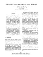
Figure 2 shows a plot of the quantity p(m) =
min{pi(rn)} as a function of m, the number of exam-
ples. Here Pi denotes the probability of being in state 1
at the end of m examples in the case where the learner
started in state i. Naturally we want
lim pi(m)=
1
and for this example this is indeed the case. The next
figure shows a plot of the following quantity as a func-
tion of m, the number of examples.
p(m) = min{pi(m)}

The quantity p(m) is easy to interpret. Thus p(m) =
0.95 rneans that for every initial state of the learner
the probability that it is in the target state after m
examples is at least 0.95. Further there is one initial
state (the worst initial state with respect to the target,
which in our example is Ls) for which this probability
is exactly 0.95. We find on looking at the curve that
the learner converges with high probability within 100
to 200 (degree-0) example sentences, a psychologically
plausible number.
We can now compare the convergence time of TLA to
other algorithms. Perhaps the simplest is random walk:
start the learner at a random point in the 3-parameter
space, and then, if an input sentence cannot be ana-
lyzed, move 1-bit randomly from state to state. Note
that this regime cannot suffer from the local maxima
problem, since there is always some finite probability of
exiting a non-target state.
Computing the convergence curves for a random walk
algorithm (RWA) on the 8 state space, we find that the
convergence times are actually faster than for the TLA;
see figure 2. Since the RWA is also superior in that it
does not suffer from the same local maxima problem
as TLA, the conceptual support for the TLA is by no
means clear. Of course, it may be that the TLA has
empirical support, in the sense of independent evidence
that children do use this procedure (given by the pat-
tern of their errors, etc.), but this evidence is lacking,
as far as we know.
DISTRIBUTIONAL ASSUMPTIONS:

PART I
In the earlier section we assumed that the data was uni-
formly distributed. We computed the transition matrix
for a particular target language and showed that con-
vergence times were of the order of 100-200 samples. In
this section we show that the convergence times depend
crucially upon the distribution. In particular we can
choose a distribution which will make the convergence
time as large as we want. Thus the distribution-free
convergence time for the 3-parameter system is infinite.
As before, we consider the situation where the target
language is L1. There are no local maxima problems
for this choice. We begin by letting the distribution be
parametrized by the variables a, b, c, d where
a = P(A = {Adv(erb)Phrase V S})
b = P(B = {Adv V O S, Adv Aux V S})
c = P(C={AdvV O1 O2S, AdvAuxVOS,
Adv Aux V O1 02 S})
d = P(D={VS})
Thus each of the sets A, B, C and D contain different
degree-O sentences of L1. Clearly the probability of the
set L, \{AUBUCUD} is 1-(a+b+c+d). The elements
of each defined subset of La are equally likely with re-
spect to each other. Setting positive values for a, b, c, d
such that a + b + c + d < 1 now defines a unique prob-
ability for each degree(O) sentence in L1. For example,
the probability of AdvVOS is b/2, the probability of
AdvAuxVOS is c/3, that of VOS is (1-(a+b+c+d))/6
and so on; see figure 3. We can now obtain the tran-
sition matrix corresponding to this distribution. If we

compare this matrix with that obtained with a uniform
distribution on the sentences of La in the earlier section.
This matrix has non-zero elements (transition proba-
bilities) exactly where the earlier matrix had non-zero
elements. However, the value of each transition prob-
ability now depends upon a,b, c, and d. In particular
if we choose a = 1/12, b = 2/12, c = 3/12, d = 1/12
(this is equivalent to assuming a uniform distribution)
we obtain the appropriate transition matrix as before.
Looking more closely at the general transition matrix,
we see that the transition probability from state 2 to
state 1 is (1- (a+b+c))/3. Clearly if we make a
arbitrarily close to 1, then this transition probability
is arbitrarily close to 0 so that the number of samples
needed to converge can be made arbitrarily large. Thus
choosing large values for a and small values for b will
result in large convergence times.
This means that the sample complexity cannot be
bounded in a distribution-free sense, because by choos-
ing a highly unfavorable distribution the sample com-
plexity can be made as high as possible. For example,
we now give the convergence curves calculated for dif-
ferent choices of a, b,c, d. We see that for a uniform
distribution the convergence occurs within 200 sam-
ples. By choosing a distribution with a = 0.9999 and
b = c = d = 0.000001, the convergence time can be
pushed up to as much as 50 million samples. (Of course,
this distribution is presumably not psychologically re-
alistic.) For a = 0.99, b = c = d = 0.0001, the sample
complexity is on the order of 100,000 positive examples.

Remark. The preceding calculation provides a worst-
case convergence time. We can also calculate average
convergence times using standard results from Markov
chain theory (see Isaacson and Madsen, 1976), as in
table 2. These support our previous results.
There are also well-known convergence theorems de-
rived from a consideration of the eigenvalues of the
transition matrix. We state without proof a conver-
gence result for transition matrices stated in terms of
its eigenvalues.
175
Table 1: Complete list of problem states, i.e., all combinations of starting grammar and target grammar which result
in non-learnability of the target. The items marked with an asterisk are those listed in the original paper by Gibson
and Wexler (1994).
Initial Grammar Target Grammar
(svo-v2)
(svo+v2)*
(soy-v2)
(SOV+V2)*
(VOS-V2)
(VOS+V2)*
(OVS-V2)
(ovs+v2)*
(vos-v2)
(VOS+V2)*
(OVS-V2)
(OVS+V2)*
(OVS-V2)
(ovs-v2)
(ovs-v2)

(ovs-v2)
(svo-v2)
(svo-v2)
(svo-v2)
(svo-v2)
(sov-v2)
(soy-v2)
(soy-v2)
(sov-v2)
State of Initial Grammar
(Markov Structure)
Not Sink
Probability of Not
Converging to Target
Not Sink
Sink
0.5
Sink
1.0
0.15
Not Sink
Sink
Not Sink
Not Sink
Not Sink
1.0
Not Sink
Sink
0.33
1.0

0.33
1.0
0.33
Sink 1.0
0.08
1.0
~f f
~m
~o
;°1
-@
6 16o 260 360 460
Number of examples (m}
Figure 2: Convergence as a function of number of examples. The probability of converging to the target state after
m examples is plotted against m. The data from the target is assumed to be distributed uniformly over degree-0
sentences. The solid line represents TLA convergence times and the dotted line is a random walk learning algorithm
(RWA) which actually converges
fasler
than the TLA in this case.
176
O
E
8
O-o
d"
,

I
i
t

t
I
t
t
t t
, /
' [
•
=, r"
o
lo 2'o 3o 4o
Log(Number of Samples)
Figure 3: Rates of convergence for TLA with
L1 as
the target language for different distributions. The probability
of converging to the target after m samples is plotted against log(m). The three curves show how unfavorable
distributions can increase convergence times. The dashed nine assumes uniform distribution and is the same curve
as plotted in figure 2.
Table 2: Mean and standard deviation convergence times to target 5 (English) given different distributions over
the target language, and a uniform distribution over initial states. The first distribution is uniform over the target
language; the other distributions
Learning Mean abs.
scenario time
TEA (uniform) 34.8
TLA (a = 0.99) 45000
TLA (a = 0.9999) 4.5 × 106
RW 9.6
alter the value of a as discussed in the main text.
Std. Dev.
of abs. time

22.3
33000
3.3 × l06
10.1
177
Theorem 2
Let T be an n x n transition matrix with
n linearly independent left eigenvectors xl xn cor-
responding to eigenvalues .~l , . . . , .~n. Let
x0
(an n-
dimensional vector) represent the starting probability of
being in each state of the chain and r be the limiting
probability of being in each state. Then after k transi-
tions, the probability of being in each state
x0T k
can be
described by
n
I1 x0T k-~ I1=11 ~ mfx0y~x, I1~<
max
I~,lk ~ II x0y,x, II
2<i<n
i=1 -
-
i=2
where the Yi's are the right eigenvectors ofT.
This theorem bounds the convergence rate to the
limiting distribution 7r (in cases where there is only
one absorption state, 7r will have a 1 corresponding to

that state and 0 everywhere else). Using this result
we bound the rates of convergence (in terms of num-
ber k of samples). It should be plain that these results
could be used to establish standard errors and confi-
dence bounds on convergence times in the usual way,
another advantage of our new approach; see table 3.
DISTRIBUTIONAL ASSUMPTIONS,
PART II
The Markov model also allows us to easily determine
the effect of distributional changes in the input. This
is important for either computer or child acquisition
studies, since we can use corpus distributions to com-
pute convergence times in advance. For instance, it
can be easily shown that convergence times depend cru-
cially upon the distribution chosen (so in particular the
TLA learning model does not follow any distribution-
free PAC results). Specifically, we can choose a distribu-
tion that will make the convergence time as large as we
want. For example, in the situation where the target
language is L1, we can increase the convergence time
arbitrarily by increasing the probability of the string
{Adv(verb) V S}. By choosing a more unfavorable dis-
tribution the convergence time can be pushed up to as
much as 50 million samples. While not surprising in it-
self, the specificity of the model allows us to be precise
about the required sample size.
CHILDES DISTRIBUTIONS
It is of interest to examine the fidelity of the model us-
ing real language distributions, namely, the CHILDES
database. We have carried out preliminary direct ex-

periments using the CHILDES caretaker English input
to "Nina" and German input to "Katrin"; these consist
of 43,612 and 632 sentences each, respectively. We note,
following well-known results by psycholinguists, that
both corpuses contain a much higher percentage of aux-
inversion and wh-questions than "ordinary" text (e.g.,
the LOB): 25,890 questions, and 11,775 wh-questions;
201 and 99 in the German corpus; but only 2,506 ques-
tions or 3.7% out of 53,495 LOB sentences.
To test convergence, an implemented system using a
newer version of deMarcken's partial parser (see deMar-
cken, 1990) analyzed each degree-0 or degree-1 sentence
as falling into one of the input patterns SVO, S Aux V,
etc., as appropriate for the target language. Sentences
not parsable into these patterns were discarded (pre-
sumably "too complex" in some sense following a tradi-
tion established by many other researchers; see Wexler
and Culicover (1980) for details). Some examples of
caretaker inputs follow:
this is a book ? what do you see in the book ?
how many rabbits ?
what is the rabbit doing ? ( )
is he hopping ? oh . and what is he playing with ?
red mir doch nicht alles nach!
ja , die schw~tzen auch immer alles nach ( )
When run through the TLA, we discover that con-
vergence falls roughly along the TLA convergence time
displayed in figure 1-roughly 100 examples to asymp-
tote. Thus, the feasibility of the basic model is con-
firmed by actual caretaker input, at least in this simple

case, for both English and German. We are contin-
uing to explore this model with other languages and
distributional assumptions. However, there is one very
important new complication that must be taken into
account: we have found that one must (obviously) add
patterns to cover the predominance of auxiliary inver-
sions and wh-questions. However, that largely begs the
question of whether the language is verb-second or not.
Thus, as far as we can tell, we have not yet arrived at
a satisfactory parameter-setting account for V2 acqui-
sition.
VARIANTS OF THE LEARNING
MODEL AND EXTENSIONS
The Markov formulation allows one to more easily ex-
plore algorithm variants. Besides the TLA, we consider
the possible three simple learning algorithm regimes by
dropping either or both of the Single Value and Greed-
iness constraints. The key result is that
ahnost any
other
regime works faster than local gradient ascent and
avoids problems with local maxima. See figure 4 for a
representative result. Thus, most interestingly, param-
eterized language learning appears particularly robust
under algorithmic changes.
EXTENSIONS, DIACHRONIC
CHANGE AND CONCLUSIONS
We remark here that the "batch" phonological param-
eter learning system of Dresher and Kaye (1990) is sus-
ceptible to a more direct PAC-type analysis, since their

system sets parameters in an "off-line" mode. We state
without proof some results that can be given in such
cases.
178
Learning scenario
TLA (uniform)
TLA(a = 0.99)
TLA(a = 0.9999)
RW
Table 3: Convergence rates derived from eigenvalue calculations.
Rate of Convergence
0(0.94 ~)
o((1- lo-~) ~)
o((1 - 10-6) k)
o(0.89 k)
q
~, d
d
,/ /
i// /'
////
L.~,
2'0 4'o 6'0 s'o 6o
Number of
samples
Figure 4: Convergence rates for different learning algorithms when L1 is the target language. The curve with the
slowest rate (large dashes) represents the TLA, the one with the fastest rate (small dashes) is the Random Walk
(RWA) with no greediness or single value constraints. Random walks with exactly one of the greediness and single
value constraints have performances in between.
179

Theorem 3 If the learner draws more than M =
1 In(l/b) samples, then it will identify the tar-
ln(l/(1-bt))
get with confidence greater than 1 - 6. ( Here bt =
P(Lt \ Uj~tLj)).
Finally, the Markov model also points to an intrigu-
ing new model for syntactic change. One simply has to
introduce two or more target languages that emit posi-
tive example strings with (probably different) frequen-
cies: each corresponding to difference language sources.
If the model is run as before, then there can be a large
probability for a learner to converge to a state different
from the highest frequency emitting target state: that
is, the learner can acquire a different parameter setting,
for example, a -V2 setting, even in a predominantly
+V2 environment. This is of course one of the histor-
ical changes that occurred in the development of En-
glish. Space does not permit us to explore all the con-
sequences of this new Markov model; we remark here
that once again we can compute convergence times and
stability under different distributions of target frequen-
cies, combining it with the usual dynamical models of
genotype fixation. In this case, the interesting result is
that the TLA actually boosts diachronic change by or-
ders of magnitude, since as observed earlier, it can per-
mit the learner to arrive at a different convergent state
even when there is just one target language emitter. In
contrast, the local maxima targets are stable, and never
undergo change. Whether this powerful "boost" effect
plays a role in diachronic change remains a topic for fu-

ture investigation. As far as we know, the possibility for
formally modeling the kind of saltation indicated by the
Markov model has not been noted previously and has
only been vaguely stated by authors such as Lightfoot
(1990).
In conclusion, by introducing a formal mathematical
model for language acquisition, we can provide rigor-
ous results on parameter learning, algorithmic varia-
tion, sample complexity, and diachronic syntax change.
These results are of interest for corpus-based acquisition
and investigations of child acquisition, as well as point-
ing the way to a more rigorous bridge between modern
computational learning theory and computational lin-
guistics.
ACKNOWLEDGMENTS
We would like to thank Ken Wexler, Ted Gibson, and
an anonymous ACL reviewer for valuable discussions
and comments on this work. Dr. Leonardo Topa pro-
vided invaluable programming assistance. All residual
errors are ours. This research is supported by NSF
grant 9217041-ASC and ARPA under the HPCC pro-
gram.
REFERENCES
Clark, Robin and Roberts, Ian (1993). "A Compu-
tational Model of Language Learnability and Lan-
guage Change." Linguistic Inquiry, 24(2):299-345.
deMarcken, Carl (1990). "Parsing the LOB Corpus."
Proceedings of the 25th Annual Meeting of the As-
sociation for Computational Linguistics. Pitts-
burgh, PA: Association for Computational Linguis-

tics, 243-251.
Dresher, Elan and Kaye, Jonathan (1990). "A Compu-
tational Learning Model For Metrical Phonology."
Cognition, 34(1):137-195.
Gibson, Edward and Wexler, Kenneth (1994). "Trig-
gers." Linguistic Inquiry, to appear.
Gold, E.M. (1967). "Language Identification in the
Limit." Information and Control, 10(4): 447-474.
Isaacson, David and Masden, John (1976). Markov
Chains. New York: John Wiley.
Lightfoot, David (1990). How to Set Parameters. Cam-
bridge, MA: MIT Press.
Wexler, Kenneth and Culicover, Peter (1980). Formal
Principles of Language Acquisition. Cambridge,
MA: MIT Press.
180