Ebook Computer organization and architecture designing for performance (Ninth edition): Part 2

PART FOUR THE CENTRAL
PROCESSING UNIT

CHAPTER

INSTRUCTION SETS:
CHARACTERISTICS AND FUNCTIONS
12.1 Machine Instruction Characteristics
Elements of a Machine Instruction
Instruction Representation
Instruction Types
Number of Addresses
Instruction Set Design
12.2 Types of Operands
Numbers
Characters
Logical Data
12.3 Intel x86 and ARM Data Types
x86 Data Types
ARM Data Types
12.4 Types of Operations
Data Transfer
Arithmetic
Logical
Conversion
Input/Output
System Control
Transfer of Control
12.5 Intel x86 and ARM Operation Types
x86 Operation Types
ARM Operation Types

12.6 Recommended Reading
12.7 Key Terms, Review Questions, and Problems
Appendix 12A Little-, Big-, and Bi-Endian

405


406

CHAPTER 12 / INSTRUCTION SETS: CHARACTERISTICS AND FUNCTIONS

LEARNING OBJECTIVES
After studying this chapter, you should be able to:
᭜
᭜
᭜
᭜
᭜
᭜

Present an overview of essential characteristics of machine instructions.
Describe the types of operands used in typical machine instruction sets.
Present an overview of x86 and ARM data types.
Describe the types of operands supported by typical machine instruction sets.
Present an overview of x86 and ARM operation types.
Understand the differences among big endian, little endian, and bi-endian.

Much of what is discussed in this book is not readily apparent to the user or
programmer of a computer. If a programmer is using a high-level language, such
as Pascal or Ada, very little of the architecture of the underlying machine is visible.

One boundary where the computer designer and the computer programmer
can view the same machine is the machine instruction set. From the designer’s point
of view, the machine instruction set provides the functional requirements for the
processor: implementing the processor is a task that in large part involves implementing the machine instruction set. The user who chooses to program in machine
language (actually, in assembly language; see Appendix B) becomes aware of the
register and memory structure, the types of data directly supported by the machine,
and the functioning of the ALU.
A description of a computer’s machine instruction set goes a long way toward
explaining the computer’s processor. Accordingly, we focus on machine instructions
in this chapter and the next.

12.1 MACHINE INSTRUCTION CHARACTERISTICS
The operation of the processor is determined by the instructions it executes,
referred to as machine instructions or computer instructions. The collection of different instructions that the processor can execute is referred to as the processor’s
instruction set.

Elements of a Machine Instruction
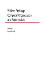
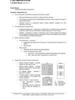
Each instruction must contain the information required by the processor for execution. Figure 12.1, which repeats Figure 3.6, shows the steps involved in instruction
execution and, by implication, defines the elements of a machine instruction. These
elements are as follows:
• Operation code: Specifies the operation to be performed (e.g., ADD, I/O).
The operation is specified by a binary code, known as the operation code, or
opcode.
• Source operand reference: The operation may involve one or more source
operands, that is, operands that are inputs for the operation.


12.1 / MACHINE INSTRUCTION CHARACTERISTICS

Operand

fetch

Instruction
fetch

Operand
store

Multiple
operands

Instruction
address
calculation

Instruction
operation
decoding

Operand
address
calculation

Instruction complete,
fetch next instruction

Figure 12.1

407

Multiple
results

Data
operation

Operand
address
calculation

Return for string
or vector data

Instruction Cycle State Diagram

• Result operand reference: The operation may produce a result.
• Next instruction reference: This tells the processor where to fetch the next
instruction after the execution of this instruction is complete.
The address of the next instruction to be fetched could be either a real address
or a virtual address, depending on the architecture. Generally, the distinction is
transparent to the instruction set architecture. In most cases, the next instruction to
be fetched immediately follows the current instruction. In those cases, there is no
explicit reference to the next instruction. When an explicit reference is needed, then
the main memory or virtual memory address must be supplied. The form in which
that address is supplied is discussed in Chapter 13.
Source and result operands can be in one of four areas:
• Main or virtual memory: As with next instruction references, the main or virtual memory address must be supplied.
• Processor register: With rare exceptions, a processor contains one or more
registers that may be referenced by machine instructions. If only one register
exists, reference to it may be implicit. If more than one register exists, then

each register is assigned a unique name or number, and the instruction must
contain the number of the desired register.
• Immediate: The value of the operand is contained in a field in the instruction
being executed.
• I/O device: The instruction must specify the I/O module and device for the
operation. If memory-mapped I/O is used, this is just another main or virtual
memory address.

Instruction Representation
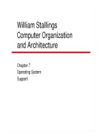
Within the computer, each instruction is represented by a sequence of bits. The
instruction is divided into fields, corresponding to the constituent elements of the


408

CHAPTER 12 / INSTRUCTION SETS: CHARACTERISTICS AND FUNCTIONS
4 Bits

6 Bits

6 Bits

Opcode

Operand reference

Operand reference

16 Bits

Figure 12.2

A Simple Instruction Format

instruction. A simple example of an instruction format is shown in Figure 12.2. As
another example, the IAS instruction format is shown in Figure 2.2. With most
instruction sets, more than one format is used. During instruction execution, an
instruction is read into an instruction register (IR) in the processor. The processor
must be able to extract the data from the various instruction fields to perform the
required operation.
It is difficult for both the programmer and the reader of textbooks to deal with
binary representations of machine instructions. Thus, it has become common practice to use a symbolic representation of machine instructions. An example of this
was used for the IAS instruction set, in Table 2.1.
Opcodes are represented by abbreviations, called mnemonics, that indicate
the operation. Common examples include
ADD

Add

SUB

Subtract

MUL

Multiply

DIV

Divide

LOAD

Load data from memory

STOR

Store data to memory

Operands are also represented symbolically. For example, the instruction
ADD R, Y
may mean add the value contained in data location Y to the contents of register R.
In this example, Y refers to the address of a location in memory, and R refers to a
particular register. Note that the operation is performed on the contents of a location, not on its address.
Thus, it is possible to write a machine-language program in symbolic form.
Each symbolic opcode has a fixed binary representation, and the programmer specifies the location of each symbolic operand. For example, the programmer might
begin with a list of definitions:
X = 513
Y = 514
and so on. A simple program would accept this symbolic input, convert opcodes and
operand references to binary form, and construct binary machine instructions.
Machine-language programmers are rare to the point of nonexistence. Most programs today are written in a high-level language or, failing that, assembly language,
which is discussed in Appendix B. However, symbolic machine language remains a
useful tool for describing machine instructions, and we will use it for that purpose.


12.1 / MACHINE INSTRUCTION CHARACTERISTICS

409

Instruction Types
Consider a high-level language instruction that could be expressed in a language
such as BASIC or FORTRAN. For example,
X = X + Y
This statement instructs the computer to add the value stored in Y to the value
stored in X and put the result in X. How might this be accomplished with machine
instructions? Let us assume that the variables X and Y correspond to locations 513
and 514. If we assume a simple set of machine instructions, this operation could be
accomplished with three instructions:
1. Load a register with the contents of memory location 513.
2. Add the contents of memory location 514 to the register.
3. Store the contents of the register in memory location 513.
As can be seen, the single BASIC instruction may require three machine
instructions. This is typical of the relationship between a high-level language and
a machine language. A high-level language expresses operations in a concise algebraic form, using variables. A machine language expresses operations in a basic
form involving the movement of data to or from registers.
With this simple example to guide us, let us consider the types of instructions
that must be included in a practical computer. A computer should have a set of
instructions that allows the user to formulate any data processing task. Another way
to view it is to consider the capabilities of a high-level programming language. Any
program written in a high-level language must be translated into machine language
to be executed. Thus, the set of machine instructions must be sufficient to express
any of the instructions from a high-level language. With this in mind we can categorize instruction types as follows:
• Data processing: Arithmetic and logic instructions
• Data storage: Movement of data into or out of register and or memory
locations
• Data movement: I/O instructions
• Control: Test and branch instructions
Arithmetic instructions provide computational capabilities for processing
numeric data. Logic (Boolean) instructions operate on the bits of a word as bits

rather than as numbers; thus, they provide capabilities for processing any other type
of data the user may wish to employ. These operations are performed primarily on
data in processor registers. Therefore, there must be memory instructions for moving data between memory and the registers. I/O instructions are needed to transfer
programs and data into memory and the results of computations back out to the
user. Test instructions are used to test the value of a data word or the status of
a computation. Branch instructions are then used to branch to a different set of
instructions depending on the decision made.
We will examine the various types of instructions in greater detail later in this
chapter.


410

CHAPTER 12 / INSTRUCTION SETS: CHARACTERISTICS AND FUNCTIONS

Number of Addresses
One of the traditional ways of describing processor architecture is in terms of the
number of addresses contained in each instruction. This dimension has become less
significant with the increasing complexity of processor design. Nevertheless, it is
useful at this point to draw and analyze this distinction.
What is the maximum number of addresses one might need in an instruction? Evidently, arithmetic and logic instructions will require the most operands.
Virtually all arithmetic and logic operations are either unary (one source operand)
or binary (two source operands). Thus, we would need a maximum of two addresses
to reference source operands. The result of an operation must be stored, suggesting
a third address, which defines a destination operand. Finally, after completion of an
instruction, the next instruction must be fetched, and its address is needed.
This line of reasoning suggests that an instruction could plausibly be required
to contain four address references: two source operands, one destination operand,
and the address of the next instruction. In most architectures, most instructions have
one, two, or three operand addresses, with the address of the next instruction being

implicit (obtained from the program counter). Most architectures also have a few
special-purpose instructions with more operands. For example, the load and store
multiple instructions of the ARM architecture, described in Chapter 13, designate
up to 17 register operands in a single instruction.
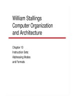
Figure 12.3 compares typical one-, two-, and three-address instructions that
could be used to compute Y = (A - B)>[C + (D * E)]. With three addresses,
each instruction specifies two source operand locations and a destination operand
location. Because we choose not to alter the value of any of the operand locations,
a temporary location, T, is used to store some intermediate results. Note that there
are four instructions and that the original expression had five operands.
Instruction
SUB Y, A, B
MPY T, D, E
ADD T, T, C
DIV
Y, Y, T

Comment
AϪB
Y
T
DϫE
T
TϩC
Y
YϬT

(a) Three-address instructions

Instruction

MOVE Y, A
SUB Y, B
MOVE T, D
MPY T, E
ADD T, C
DIV
Y, T

Comment
A
YϪB
D
TϫE
TϩC
YϬT

Y
Y
T
T
T
Y

(b) Two-address instructions

Figure 12.3

Programs to Execute Y =

Instruction

Comment

LOAD
MPY
ADD
STOR
LOAD
SUB
DIV
STOR

D
AC
AC
AC ϫ E
AC
AC ϩ C
Y
AC
AC
A
AC
AC Ϫ B
AC
AC Ϭ Y
Y
AC

D

E
C
Y
A
B
Y
Y

(c) One-address instructions

A - B
C + (D * E)


12.1 / MACHINE INSTRUCTION CHARACTERISTICS

411

Three-address instruction formats are not common because they require a
relatively long instruction format to hold the three address references. With twoaddress instructions, and for binary operations, one address must do double duty as
both an operand and a result. Thus, the instruction SUB Y, B carries out the calculation Y - B and stores the result in Y. The two-address format reduces the space
requirement but also introduces some awkwardness. To avoid altering the value of
an operand, a MOVE instruction is used to move one of the values to a result or
temporary location before performing the operation. Our sample program expands
to six instructions.
Simpler yet is the one-address instruction. For this to work, a second address
must be implicit. This was common in earlier machines, with the implied address
being a processor register known as the accumulator (AC). The accumulator contains one of the operands and is used to store the result. In our example, eight
instructions are needed to accomplish the task.
It is, in fact, possible to make do with zero addresses for some instructions.

Zero-address instructions are applicable to a special memory organization called
a stack. A stack is a last-in-first-out set of locations. The stack is in a known location and, often, at least the top two elements are in processor registers. Thus,
zero-address instructions would reference the top two stack elements. Stacks are
described in Appendix O. Their use is explored further later in this chapter and in
Chapter 13.
Table 12.1 summarizes the interpretations to be placed on instructions with
zero, one, two, or three addresses. In each case in the table, it is assumed that the
address of the next instruction is implicit, and that one operation with two source
operands and one result operand is to be performed.
The number of addresses per instruction is a basic design decision. Fewer
addresses per instruction result in instructions that are more primitive, requiring a
less complex processor. It also results in instructions of shorter length. On the other
hand, programs contain more total instructions, which in general results in longer
execution times and longer, more complex programs. Also, there is an important
threshold between one-address and multiple-address instructions. With one-address
instructions, the programmer generally has available only one general-purpose register, the accumulator. With multiple-address instructions, it is common to have
multiple general-purpose registers. This allows some operations to be performed

Table 12.1

Utilization of Instruction Addresses (Nonbranching Instructions)

Number of Addresses

AC
T
(T - 1)
A, B, C

=

=
=
=

Symbolic Representation

Interpretation

3

OP A, B, C

A d B OP C

2

OP A, B

A d A OP B

1

OP A

AC d AC OP A

0

OP

T d (T - 1) OP T

accumulator
top of stack
second element of stack
memory or register locations


412

CHAPTER 12 / INSTRUCTION SETS: CHARACTERISTICS AND FUNCTIONS

solely on registers. Because register references are faster than memory references,
this speeds up execution. For reasons of flexibility and ability to use multiple registers, most contemporary machines employ a mixture of two- and three-address
instructions.
The design trade-offs involved in choosing the number of addresses per instruction are complicated by other factors. There is the issue of whether an address references a memory location or a register. Because there are fewer registers, fewer bits
are needed for a register reference. Also, as we shall see in Chapter 13, a machine
may offer a variety of addressing modes, and the specification of mode takes one or
more bits. The result is that most processor designs involve a variety of instruction
formats.

Instruction Set Design
One of the most interesting, and most analyzed, aspects of computer design is
instruction set design. The design of an instruction set is very complex because it
affects so many aspects of the computer system. The instruction set defines many
of the functions performed by the processor and thus has a significant effect on the
implementation of the processor. The instruction set is the programmer’s means of
controlling the processor. Thus, programmer requirements must be considered in
designing the instruction set.
It may surprise you to know that some of the most fundamental issues relating to the design of instruction sets remain in dispute. Indeed, in recent years, the

level of disagreement concerning these fundamentals has actually grown. The most
important of these fundamental design issues include the following:
• Operation repertoire: How many and which operations to provide, and how
complex operations should be
• Data types: The various types of data upon which operations are performed
• Instruction format: Instruction length (in bits), number of addresses, size of
various fields, and so on
• Registers: Number of processor registers that can be referenced by instructions, and their use
• Addressing: The mode or modes by which the address of an operand is
specified
These issues are highly interrelated and must be considered together in designing an instruction set. This book, of course, must consider them in some sequence,
but an attempt is made to show the interrelationships.
Because of the importance of this topic, much of Part Three is devoted to
instruction set design. Following this overview section, this chapter examines data
types and operation repertoire. Chapter 13 examines addressing modes (which
includes a consideration of registers) and instruction formats. Chapter 15 examines
the reduced instruction set computer (RISC). RISC architecture calls into question many of the instruction set design decisions traditionally made in commercial
computers.


12.2 / TYPES OF OPERANDS

413

12.2 TYPES OF OPERANDS
Machine instructions operate on data. The most important general categories of
data are
•
•
•

•

Addresses
Numbers
Characters
Logical data

We shall see, in discussing addressing modes in Chapter 13, that addresses
are, in fact, a form of data. In many cases, some calculation must be performed on
the operand reference in an instruction to determine the main or virtual memory
address. In this context, addresses can be considered to be unsigned integers.
Other common data types are numbers, characters, and logical data, and each
of these is briefly examined in this section. Beyond that, some machines define specialized data types or data structures. For example, there may be machine operations that operate directly on a list or a string of characters.

Numbers
All machine languages include numeric data types. Even in nonnumeric data processing, there is a need for numbers to act as counters, field widths, and so forth.
An important distinction between numbers used in ordinary mathematics and numbers stored in a computer is that the latter are limited. This is true in two senses.
First, there is a limit to the magnitude of numbers representable on a machine and
second, in the case of floating-point numbers, a limit to their precision. Thus, the
programmer is faced with understanding the consequences of rounding, overflow,
and underflow.
Three types of numerical data are common in computers:
• Binary integer or binary fixed point
• Binary floating point
• Decimal
We examined the first two in some detail in Chapter 10. It remains to say a few
words about decimal numbers.
Although all internal computer operations are binary in nature, the human
users of the system deal with decimal numbers. Thus, there is a necessity to convert
from decimal to binary on input and from binary to decimal on output. For applications in which there is a great deal of I/O and comparatively little, comparatively

simple computation, it is preferable to store and operate on the numbers in decimal
form. The most common representation for this purpose is packed decimal.1
1

Textbooks often refer to this as binary coded decimal (BCD). Strictly speaking, BCD refers to the
encoding of each decimal digit by a unique 4-bit sequence. Packed decimal refers to the storage of BCDencoded digits using one byte for each two digits.


414

CHAPTER 12 / INSTRUCTION SETS: CHARACTERISTICS AND FUNCTIONS

With packed decimal, each decimal digit is represented by a 4-bit code, in the
obvious way, with two digits stored per byte. Thus, 0 = 000, 1 = 0001, c, 8 = 1000,
and 9 = 1001. Note that this is a rather inefficient code because only 10 of 16 possible 4-bit values are used. To form numbers, 4-bit codes are strung together, usually in multiples of 8 bits. Thus, the code for 246 is 0000 0010 0100 0110. This code
is clearly less compact than a straight binary representation, but it avoids the conversion overhead. Negative numbers can be represented by including a 4-bit sign
digit at either the left or right end of a string of packed decimal digits. Standard sign
values are 1100 for positive ( + ) and 1101 for negative ( - ).
Many machines provide arithmetic instructions for performing operations
directly on packed decimal numbers. The algorithms are quite similar to those
described in Section 9.3 but must take into account the decimal carry operation.

Characters
A common form of data is text or character strings. While textual data are most
convenient for human beings, they cannot, in character form, be easily stored or
transmitted by data processing and communications systems. Such systems are
designed for binary data. Thus, a number of codes have been devised by which characters are represented by a sequence of bits. Perhaps the earliest common example
of this is the Morse code. Today, the most commonly used character code in the
International Reference Alphabet (IRA), referred to in the United States as the
American Standard Code for Information Interchange (ASCII; see Appendix F).

Each character in this code is represented by a unique 7-bit pattern; thus, 128 different characters can be represented. This is a larger number than is necessary to
represent printable characters, and some of the patterns represent control characters. Some of these control characters have to do with controlling the printing
of characters on a page. Others are concerned with communications procedures.
IRA-encoded characters are almost always stored and transmitted using 8 bits per
character. The eighth bit may be set to 0 or used as a parity bit for error detection.
In the latter case, the bit is set such that the total number of binary 1s in each octet
is always odd (odd parity) or always even (even parity).
Note in Table F.1 (Appendix F) that for the IRA bit pattern 011XXXX, the
digits 0 through 9 are represented by their binary equivalents, 0000 through 1001, in
the rightmost 4 bits. This is the same code as packed decimal. This facilitates conversion between 7-bit IRA and 4-bit packed decimal representation.
Another code used to encode characters is the Extended Binary Coded
Decimal Interchange Code (EBCDIC). EBCDIC is used on IBM mainframes. It
is an 8-bit code. As with IRA, EBCDIC is compatible with packed decimal. In
the case of EBCDIC, the codes 11110000 through 11111001 represent the digits
0 through 9.

Logical Data
Normally, each word or other addressable unit (byte, halfword, and so on) is treated
as a single unit of data. It is sometimes useful, however, to consider an n-bit unit as
consisting of n 1-bit items of data, each item having the value 0 or 1. When data are
viewed this way, they are considered to be logical data.


12.3 / INTEL x86 AND ARM DATA TYPES

415

There are two advantages to the bit-oriented view. First, we may sometimes wish
to store an array of Boolean or binary data items, in which each item can take on only
the values 1 (true) and 0 (false). With logical data, memory can be used most efficiently

for this storage. Second, there are occasions when we wish to manipulate the bits of a
data item. For example, if floating-point operations are implemented in software, we
need to be able to shift significant bits in some operations. Another example: To convert from IRA to packed decimal, we need to extract the rightmost 4 bits of each byte.
Note that, in the preceding examples, the same data are treated sometimes as
logical and other times as numerical or text. The “type” of a unit of data is determined by the operation being performed on it. While this is not normally the case in
high-level languages, it is almost always the case with machine language.

12.3 INTEL x86 AND ARM DATA TYPES
x86 Data Types
The x86 can deal with data types of 8 (byte), 16 (word), 32 (doubleword), 64 (quadword), and 128 (double quadword) bits in length. To allow maximum flexibility in
data structures and efficient memory utilization, words need not be aligned at evennumbered addresses; doublewords need not be aligned at addresses evenly divisible
by 4; and quadwords need not be aligned at addresses evenly divisible by 8; and
so on. However, when data are accessed across a 32-bit bus, data transfers take
place in units of doublewords, beginning at addresses divisible by 4. The processor
converts the request for misaligned values into a sequence of requests for the bus
transfer. As with all of the Intel 80x86 machines, the x86 uses the little-endian style;
that is, the least significant byte is stored in the lowest address (see Appendix 12A
for a discussion of endianness).
The byte, word, doubleword, quadword, and double quadword are referred to
as general data types. In addition, the x86 supports an impressive array of specific
data types that are recognized and operated on by particular instructions. Table 12.2
summarizes these types.
Figure 12.4 illustrates the x86 numerical data types. The signed integers are in
twos complement representation and may be 16, 32, or 64 bits long. The floatingpoint type actually refers to a set of types that are used by the floating-point unit
and operated on by floating-point instructions. The three floating-point representations conform to the IEEE 754 standard.
The packed SIMD (single-instruction-multiple-data) data types were introduced to the x86 architecture as part of the extensions of the instruction set to
optimize performance of multimedia applications. These extensions include MMX
(multimedia extensions) and SSE (streaming SIMD extensions). The basic concept
is that multiple operands are packed into a single referenced memory item and that
these multiple operands are operated on in parallel. The data types are as follows:

• Packed byte and packed byte integer: Bytes packed into a 64-bit quadword or
128-bit double quadword, interpreted as a bit field or as an integer
• Packed word and packed word integer: 16-bit words packed into a 64-bit quadword or 128-bit double quadword, interpreted as a bit field or as an integer


416

CHAPTER 12 / INSTRUCTION SETS: CHARACTERISTICS AND FUNCTIONS

Table 12.2

x86 Data Types

Data Type

Description

General

Byte, word (16 bits), doubleword (32 bits), quadword (64 bits), and
double quadword (128 bits) locations with arbitrary binary contents.

Integer

A signed binary value contained in a byte, word, or doubleword, using
twos complement representation.

Ordinal

An unsigned integer contained in a byte, word, or doubleword.

Unpacked binary coded
decimal (BCD)

A representation of a BCD digit in the range 0 through 9, with one
digit in each byte.

Packed BCD

Packed byte representation of two BCD digits; value in the range 0 to 99.

Near pointer

A 16-bit, 32-bit, or 64-bit effective address that represents the offset
within a segment. Used for all pointers in a nonsegmented memory and
for references within a segment in a segmented memory.

Far pointer

A logical address consisting of a 16-bit segment selector and an offset
of 16, 32, or 64 bits. Far pointers are used for memory references in a
segmented memory model where the identity of a segment being
accessed must be specified explicitly.

Bit field

A contiguous sequence of bits in which the position of each bit is
considered as an independent unit. A bit string can begin at any bit
position of any byte and can contain up to 32 bits.

Bit string

A contiguous sequence of bits, containing from zero to 232 - 1 bits.

Byte string

A contiguous sequence of bytes, words, or doublewords, containing from
zero to 232 - 1 bytes.

Floating point

See Figure 12.4.

Packed SIMD (single
instruction, multiple data)

Packed 64-bit and 128-bit data types

• Packed doubleword and packed doubleword integer: 32-bit doublewords
packed into a 64-bit quadword or 128-bit double quadword, interpreted as a
bit field or as an integer
• Packed quadword and packed qaudword integer: Two 64-bit quadwords
packed into a 128-bit double quadword, interpreted as a bit field or as an integer
• Packed single-precision floating-point and packed double-precision floatingpoint: Four 32-bit floating-point or two 64-bit floating-point values packed
into a 128-bit double quadword

ARM Data Types
ARM processors support data types of 8 (byte), 16 (halfword), and 32 (word) bits
in length. Normally, halfword access should be halfword aligned and word accesses
should be word aligned. For nonaligned access attempts, the architecture supports

three alternatives.
• Default case:
– The address is treated as truncated, with address bits[1:0] treated as zero
for word accesses, and address bit[0] treated as zero for halfword accesses.


12.3 / INTEL x86 AND ARM DATA TYPES

417

Byte unsigned integer
7

0
Word unsigned integer

15

0
Doubleword unsigned integer

31

0
Quadword unsigned integer

63

0
Byte signed integer

Twos comp
7

0

Twos comp Word unsigned integer
15

0
Doubleword unsigned integer

Twos complement
0

31

Quadword unsigned integer

Twos complement
63

Sign bit
Exp
63
51
Sign bit
Integer bit
Exponent
79

Figure 12.4

Sign bit
Exp

0
Single precision
floating point

Significand

31

0
Double precision
Floating point

Significand
0

Double extended precision
floating point

Significand

63

0

x86 Numeric Data Formats

– Load single word ARM instructions are architecturally defined to rotate right
the word-aligned data transferred by a non word-aligned address one, two, or
three bytes depending on the value of the two least significant address bits.
• Alignment checking: When the appropriate control bit is set, a data abort signal indicates an alignment fault for attempting unaligned access.
• Unaligned access: When this option is enabled, the processor uses one or more
memory accesses to generate the required transfer of adjacent bytes transparently to the programmer.
For all three data types (byte, halfword, and word) an unsigned interpretation
is supported, in which the value represents an unsigned, nonnegative integer. All
three data types can also be used for twos complement signed integers.
The majority of ARM processor implementations do not provide floatingpoint hardware, which saves power and area. If floating-point arithmetic is required
in such processors, it must be implemented in software. ARM does support an
optional floating-point coprocessor that supports the single- and double-precision
floating point data types defined in IEEE 754.


418

CHAPTER 12 / INSTRUCTION SETS: CHARACTERISTICS AND FUNCTIONS
Data bytes
in memory
(ascending address values
from byte 0 to byte 3)
Byte 3
Byte 2
Byte 1
Byte 0

31

0

Byte 3

Byte 2

Byte 1

Byte 0

31

0

Byte 0

Byte 1

Byte 2

Byte 3

ARM register

ARM register

Program status register E-bit = 0

Program status register E-bit = 1

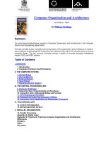
Figure 12.5

ARM Endian Support—Word Load/Store with E-Bit

ENDIAN SUPPORT A state bit (E-bit) in the system control register is set and cleared

under program control using the SETEND instruction. The E-bit defines which
endian to load and store data. Figure 12.5 illustrates the functionality associated
with the E-bit for a word load or store operation. This mechanism enables efficient
dynamic data load/store for system designers who know they need to access data
structures in the opposite endianness to their OS/environment. Note that the address
of each data byte is fixed in memory. However, the byte lane in a register is different.

12.4 TYPES OF OPERATIONS
The number of different opcodes varies widely from machine to machine. However,
the same general types of operations are found on all machines. A useful and typical
categorization is the following:
•
•
•
•
•
•
•

Data transfer
Arithmetic
Logical
Conversion

I/O
System control
Transfer of control

Table 12.3 (based on [HAYE98]) lists common instruction types in each category. This section provides a brief survey of these various types of operations,
together with a brief discussion of the actions taken by the processor to execute a
particular type of operation (summarized in Table 12.4). The latter topic is examined
in more detail in Chapter 14.


12.4 / TYPES OF OPERATIONS
Table 12.3

419

Common Instruction Set Operations

Type

Data transfer

Arithmetic

Logical

Operation Name

Description

Move (transfer)

Transfer word or block from source to destination

Store

Transfer word from processor to memory

Load (fetch)

Transfer word from memory to processor

Exchange

Swap contents of source and destination

Clear (reset)

Transfer word of 0s to destination

Set

Transfer word of 1s to destination

Push

Transfer word from source to top of stack

Pop

Transfer word from top of stack to destination

Add

Compute sum of two operands

Subtract

Compute difference of two operands

Multiply

Compute product of two operands

Divide

Compute quotient of two operands

Absolute

Replace operand by its absolute value

Negate

Change sign of operand

Increment

Add 1 to operand

Decrement

Subtract 1 from operand

AND

Perform logical AND

OR

Perform logical OR

NOT (complement)

Perform logical NOT

Exclusive-OR

Perform logical XOR

Test

Test specified condition; set flag(s) based on outcome

Compare

Make logical or arithmetic comparison of two or more
operands; set flag(s) based on outcome

Set Control Variables

Class of instructions to set controls for protection
purposes, interrupt handling, timer control, etc.

Shift

Left (right) shift operand, introducing constants at end

Rotate

Left (right) shift operand, with wraparound end

Jump (branch)

Unconditional transfer; load PC with specified address

Jump Conditional

Test specified condition; either load PC with specified
address or do nothing, based on condition

Jump to Subroutine

Place current program control information in known
location; jump to specified address

Return

Replace contents of PC and other register from known location

Execute

Fetch operand from specified location and execute as
instruction; do not modify PC

Skip

Increment PC to skip next instruction

Skip Conditional

Test specified condition; either skip or do nothing based
on condition

Halt

Stop program execution

Wait (hold)

Stop program execution; test specified condition repeatedly;
resume execution when condition is satisfied

No operation

No operation is performed, but program execution is continued

Transfer of control

(continued)

420

CHAPTER 12 / INSTRUCTION SETS: CHARACTERISTICS AND FUNCTIONS

Table 12.3

Continued

Type

Operation Name

Input/output

Input (read)

Transfer data from specified I/O port or device to destination
(e.g., main memory or processor register)

Output (write)

Transfer data from specified source to I/O port or device

Start I/O

Transfer instructions to I/O processor to initiate I/O operation

Test I/O

Transfer status information from I/O system to specified
destination

Translate

Translate values in a section of memory based on a table
of correspondences

Convert

Convert the contents of a word from one form to another
(e.g., packed decimal to binary)

Conversion

Table 12.4

Description

Processor Actions for Various Types of Operations
Transfer data from one location to another

Data transfer

If memory is involved:
Determine memory address
Perform virtual-to-actual-memory address transformation
Check cache
Initiate memory read/write
May involve data transfer, before and/or after

Arithmetic

Perform function in ALU
Set condition codes and flags

Logical

Same as arithmetic

Conversion

Similar to arithmetic and logical. May involve special logic to perform
conversion

Transfer of control

Update program counter. For subroutine call/return, manage parameter
passing and linkage
Issue command to I/O module

I/O

If memory-mapped I/O, determine memory-mapped address

Data Transfer
The most fundamental type of machine instruction is the data transfer instruction.
The data transfer instruction must specify several things. First, the location of the
source and destination operands must be specified. Each location could be memory,
a register, or the top of the stack. Second, the length of data to be transferred must

be indicated. Third, as with all instructions with operands, the mode of addressing
for each operand must be specified. This latter point is discussed in Chapter 13.
The choice of data transfer instructions to include in an instruction set exemplifies the kinds of trade-offs the designer must make. For example, the general
location (memory or register) of an operand can be indicated in either the specification of the opcode or the operand. Table 12.5 shows examples of the most common
IBM EAS/390 data transfer instructions. Note that there are variants to indicate


12.4 / TYPES OF OPERATIONS
Table 12.5
Operation
Mnemonic

421

Examples of IBM EAS/390 Data Transfer Operations
Name

Number of Bits
Transferred

Description

L

Load

32

Transfer from memory to register

LH

Load Halfword

16

Transfer from memory to register

LR

Load

32

Transfer from register to register

LER

Load (short)

32

Transfer from floating-point register to
floating-point register

LE

Load (short)

32

Transfer from memory to floating-point
register

LDR

Load (long)

64

Transfer from floating-point register to
floating-point register

LD

Load (long)

64

Transfer from memory to floating-point
register

ST

Store

32

Transfer from register to memory

STH

Store Halfword

16

Transfer from register to memory

STC

Store Character

8

Transfer from register to memory

STE

Store (short)

32

Transfer from floating-point register to
memory

STD

Store (long)

64

Transfer from floating-point register to
memory

the amount of data to be transferred (8, 16, 32, or 64 bits). Also, there are different
instructions for register to register, register to memory, memory to register, and
memory to memory transfers. In contrast, the VAX has a move (MOV) instruction
with variants for different amounts of data to be moved, but it specifies whether an
operand is register or memory as part of the operand. The VAX approach is somewhat easier for the programmer, who has fewer mnemonics to deal with. However,
it is also somewhat less compact than the IBM EAS/390 approach because the location (register versus memory) of each operand must be specified separately in the
instruction. We will return to this distinction when we discuss instruction formats in
Chapter 13.
In terms of processor action, data transfer operations are perhaps the simplest
type. If both source and destination are registers, then the processor simply causes
data to be transferred from one register to another; this is an operation internal to
the processor. If one or both operands are in memory, then the processor must perform some or all of the following actions:
1. Calculate the memory address, based on the address mode (discussed in
Chapter 13).
2. If the address refers to virtual memory, translate from virtual to real memory
address.
3. Determine whether the addressed item is in cache.
4. If not, issue a command to the memory module.


422

CHAPTER 12 / INSTRUCTION SETS: CHARACTERISTICS AND FUNCTIONS

Arithmetic
Most machines provide the basic arithmetic operations of add, subtract, multiply, and divide. These are invariably provided for signed integer (fixed-point)

numbers. Often they are also provided for floating-point and packed decimal
numbers.
Other possible operations include a variety of single-operand instructions; for
example,
•
•
•
•

Absolute: Take the absolute value of the operand.
Negate: Negate the operand.
Increment: Add 1 to the operand.
Decrement: Subtract 1 from the operand.

The execution of an arithmetic instruction may involve data transfer operations to position operands for input to the ALU, and to deliver the output of the
ALU. Figure 3.5 illustrates the movements involved in both data transfer and arithmetic operations. In addition, of course, the ALU portion of the processor performs
the desired operation.

Logical
Most machines also provide a variety of operations for manipulating individual bits
of a word or other addressable units, often referred to as “bit twiddling.” They are
based upon Boolean operations (see Chapter 11).
Some of the basic logical operations that can be performed on Boolean or
binary data are shown in Table 12.6. The NOT operation inverts a bit. AND, OR,
and Exclusive-OR (XOR) are the most common logical functions with two operands. EQUAL is a useful binary test.
These logical operations can be applied bitwise to n-bit logical data units.
Thus, if two registers contain the data
(R1) = 10100101
(R2) = 00001111
then

(R1) AND (R2) = 00000101

Table 12.6

Basic Logical Operations

P

Q

NOT P

P AND Q

P OR Q

P XOR Q

P ‫ ؍‬Q

0

0

1

0

0

0

1

0

1

1

0

1

1

0

1

0

0

0

1

1

0

1

1

0

1

1

0

1


12.4 / TYPES OF OPERATIONS

423

where the notation (X) means the contents of location X. Thus, the AND operation
can be used as a mask that selects certain bits in a word and zeros out the remaining
bits. As another example, if two registers contain
(R1) = 10100101
(R2) = 11111111
then
(R1) XOR (R2) = 01011010
With one word set to all 1s, the XOR operation inverts all of the bits in the other
word (ones complement).

In addition to bitwise logical operations, most machines provide a variety of
shifting and rotating functions. The most basic operations are illustrated in Figure 12.6.
With a logical shift, the bits of a word are shifted left or right. On one end, the bit
shifted out is lost. On the other end, a 0 is shifted in. Logical shifts are useful primarily for isolating fields within a word. The 0s that are shifted into a word displace
unwanted information that is shifted off the other end.
0
• • •
(a) Logical right shift
0
• • •
(b) Logical left shift

S

• • •
(c) Arithmetic right shift
0

S

• • •
(d) Arithmetic left shift

• • •
(e) Right rotate

• • •
(f) Left rotate

Figure 12.6

Shift and Rotate Operations


424

CHAPTER 12 / INSTRUCTION SETS: CHARACTERISTICS AND FUNCTIONS

As an example, suppose we wish to transmit characters of data to an I/O
device 1 character at a time. If each memory word is 16 bits in length and contains
two characters, we must unpack the characters before they can be sent. To send the
two characters in a word,
1. Load the word into a register.
2. Shift to the right eight times. This shifts the remaining character to the right
half of the register.
3. Perform I/O. The I/O module reads the lower-order 8 bits from the data bus.
The preceding steps result in sending the left-hand character. To send the righthand character,
1. Load the word again into the register.
2. AND with 0000000011111111. This masks out the character on the left.
3. Perform I/O.
The arithmetic shift operation treats the data as a signed integer and does
not shift the sign bit. On a right arithmetic shift, the sign bit is replicated into the
bit position to its right. On a left arithmetic shift, a logical left shift is performed on
all bits but the sign bit, which is retained. These operations can speed up certain
arithmetic operations. With numbers in twos complement notation, a right arithmetic shift corresponds to a division by 2, with truncation for odd numbers. Both an
arithmetic left shift and a logical left shift correspond to a multiplication by 2 when
there is no overflow. If overflow occurs, arithmetic and logical left shift operations
produce different results, but the arithmetic left shift retains the sign of the number.
Because of the potential for overflow, many processors do not include this instruction, including PowerPC and Itanium. Others, such as the IBM EAS/390, do offer
the instruction. Curiously, the x86 architecture includes an arithmetic left shift but

defines it to be identical to a logical left shift.
Rotate, or cyclic shift, operations preserve all of the bits being operated on.
One use of a rotate is to bring each bit successively into the leftmost bit, where it can
be identified by testing the sign of the data (treated as a number).
As with arithmetic operations, logical operations involve ALU activity and
may involve data transfer operations. Table 12.7 gives examples of all of the shift
and rotate operations discussed in this subsection.
Table 12.7
Input

Examples of Shift and Rotate Operations
Operation

Result

10100110

Logical right shift (3 bits)

00010100

10100110

Logical left shift (3 bits)

00110000

10100110

Arithmetic right shift (3 bits)

11110100

10100110

Arithmetic left shift (3 bits)

10110000

10100110

Right rotate (3 bits)

11010100

10100110

Left rotate (3 bits)

00110101


12.4 / TYPES OF OPERATIONS

425

Conversion
Conversion instructions are those that change the format or operate on the format of
data. An example is converting from decimal to binary. An example of a more complex editing instruction is the EAS/390 Translate (TR) instruction. This instruction
can be used to convert from one 8-bit code to another, and it takes three operands:

TR R1 (L), R2
The operand R2 contains the address of the start of a table of 8-bit codes. The
L bytes starting at the address specified in R1 are translated, each byte being
replaced by the contents of a table entry indexed by that byte. For example, to
translate from EBCDIC to IRA, we first create a 256-byte table in storage locations, say, 1000-10FF hexadecimal. The table contains the characters of the IRA
code in the sequence of the binary representation of the EBCDIC code; that is, the
IRA code is placed in the table at the relative location equal to the binary value of
the EBCDIC code of the same character. Thus, locations 10F0 through 10F9 will
contain the values 30 through 39, because F0 is the EBCDIC code for the digit 0,
and 30 is the IRA code for the digit 0, and so on through digit 9. Now suppose we
have the EBCDIC for the digits 1984 starting at location 2100 and we wish to translate to IRA. Assume the following:
• Locations 2100–2103 contain F1 F9 F8 F4.
• R1 contains 2100.
• R2 contains 1000.
Then, if we execute
TR R1 (4), R2
locations 2100–2103 will contain 31 39 38 34.

Input/Output
Input/output instructions were discussed in some detail in Chapter 7. As we saw,
there are a variety of approaches taken, including isolated programmed I/O,
memory-mapped programmed I/O, DMA, and the use of an I/O processor. Many
implementations provide only a few I/O instructions, with the specific actions specified by parameters, codes, or command words.

System Control
System control instructions are those that can be executed only while the processor
is in a certain privileged state or is executing a program in a special privileged area
of memory. Typically, these instructions are reserved for the use of the operating
system.
Some examples of system control operations are as follows. A system control instruction may read or alter a control register; we discuss control registers in

Chapter 14. Another example is an instruction to read or modify a storage protection key, such as is used in the EAS/390 memory system. Another example is access
to process control blocks in a multiprogramming system.


426

CHAPTER 12 / INSTRUCTION SETS: CHARACTERISTICS AND FUNCTIONS

Transfer of Control
For all of the operation types discussed so far, the next instruction to be performed
is the one that immediately follows, in memory, the current instruction. However, a
significant fraction of the instructions in any program have as their function changing the sequence of instruction execution. For these instructions, the operation performed by the processor is to update the program counter to contain the address of
some instruction in memory.
There are a number of reasons why transfer-of-control operations are
required. Among the most important are the following:
1. In the practical use of computers, it is essential to be able to execute each
instruction more than once and perhaps many thousands of times. It may
require thousands or perhaps millions of instructions to implement an application. This would be unthinkable if each instruction had to be written out separately. If a table or a list of items is to be processed, a program loop is needed.
One sequence of instructions is executed repeatedly to process all the data.
2. Virtually all programs involve some decision making. We would like the computer to do one thing if one condition holds, and another thing if another condition
holds. For example, a sequence of instructions computes the square root of a number. At the start of the sequence, the sign of the number is tested. If the number
is negative, the computation is not performed, but an error condition is reported.
3. To compose correctly a large or even medium-size computer program is an
exceedingly difficult task. It helps if there are mechanisms for breaking the
task up into smaller pieces that can be worked on one at a time.
We now turn to a discussion of the most common transfer-of-control operations found in instruction sets: branch, skip, and procedure call.
BRANCH INSTRUCTIONS A branch instruction, also called a jump instruction,
has as one of its operands the address of the next instruction to be executed. Most
often, the instruction is a conditional branch instruction. That is, the branch is made
(update program counter to equal address specified in operand) only if a certain

condition is met. Otherwise, the next instruction in sequence is executed (increment
program counter as usual). A branch instruction in which the branch is always taken
is an unconditional branch.
There are two common ways of generating the condition to be tested in a conditional branch instruction. First, most machines provide a 1-bit or multiple-bit condition code that is set as the result of some operations. This code can be thought
of as a short user-visible register. As an example, an arithmetic operation (ADD,
SUBTRACT, and so on) could set a 2-bit condition code with one of the following
four values: 0, positive, negative, overflow. On such a machine, there could be four
different conditional branch instructions:

BRP X
BRN X
BRZ X
BRO X

Branch to location X if result is positive.
Branch to location X if result is negative.
Branch to location X if result is zero.
Branch to location X if overflow occurs.


12.4 / TYPES OF OPERATIONS

Unconditional
branch

Memory
address

Instruction

200
201
202
203

SUB X,Y
BRZ 211

210
211

BR 202

225

BRE R1, R2, 235

427

Conditional
branch

Conditional
branch
235

Figure 12.7

Branch Instructions

In all of these cases, the result referred to is the result of the most recent
operation that set the condition code.
Another approach that can be used with a three-address instruction format is
to perform a comparison and specify a branch in the same instruction. For example,
BRE R1, R2, X

Branch to X if contents of R1 = contents of R2.

Figure 12.7 shows examples of these operations. Note that a branch can be
either forward (an instruction with a higher address) or backward (lower address).
The example shows how an unconditional and a conditional branch can be used to
create a repeating loop of instructions. The instructions in locations 202 through 210
will be executed repeatedly until the result of subtracting Y from X is 0.
SKIP INSTRUCTIONS Another form of transfer-of-control instruction is the skip

instruction. The skip instruction includes an implied address. Typically, the skip
implies that one instruction be skipped; thus, the implied address equals the address
of the next instruction plus one instruction length.
Because the skip instruction does not require a destination address field, it is
free to do other things. A typical example is the increment-and-skip-if-zero (ISZ)
instruction. Consider the following program fragment:
301
~
~
~
309 ISZ R1
310 BR 301
311
In this fragment, the two transfer-of-control instructions are used to implement
an iterative loop. R1 is set with the negative of the number of iterations to be

performed. At the end of the loop, R1 is incremented. If it is not 0, the program
branches back to the beginning of the loop. Otherwise, the branch is skipped, and
the program continues with the next instruction after the end of the loop.


428

CHAPTER 12 / INSTRUCTION SETS: CHARACTERISTICS AND FUNCTIONS
PROCEDURE CALL INSTRUCTIONS Perhaps the most important innovation in the

development of programming languages is the procedure. A procedure is a selfcontained computer program that is incorporated into a larger program. At any
point in the program the procedure may be invoked, or called. The processor is
instructed to go and execute the entire procedure and then return to the point from
which the call took place.
The two principal reasons for the use of procedures are economy and modularity. A procedure allows the same piece of code to be used many times. This is
important for economy in programming effort and for making the most efficient use
of storage space in the system (the program must be stored). Procedures also allow
large programming tasks to be subdivided into smaller units. This use of modularity
greatly eases the programming task.
The procedure mechanism involves two basic instructions: a call instruction
that branches from the present location to the procedure, and a return instruction
that returns from the procedure to the place from which it was called. Both of these
are forms of branching instructions.
Figure 12.8a illustrates the use of procedures to construct a program. In this
example, there is a main program starting at location 4000. This program includes
a call to procedure PROC1, starting at location 4500. When this call instruction is
encountered, the processor suspends execution of the main program and begins execution of PROC1 by fetching the next instruction from location 4500. Within PROC1,
there are two calls to PROC2 at location 4800. In each case, the execution of PROC1
Addresses

Main memory

4000
4100
4101

CALL Proc1

Main
program

4500
4600
4601

CALL Proc2

4650
4651

CALL Proc2

Procedure
Proc1

RETURN

4800
Procedure
Proc2

RETURN
(a) Calls and returns

Figure 12.8

Nested Procedures

(b) Execution sequence


12.4 / TYPES OF OPERATIONS

429

is suspended and PROC2 is executed. The RETURN statement causes the processor to go back to the calling program and continue execution at the instruction after
the corresponding CALL instruction. This behavior is illustrated in Figure 12.8b.
Three points are worth noting:
1. A procedure can be called from more than one location.
2. A procedure call can appear in a procedure. This allows the nesting of procedures to an arbitrary depth.
3. Each procedure call is matched by a return in the called program.
Because we would like to be able to call a procedure from a variety of points,
the processor must somehow save the return address so that the return can take
place appropriately. There are three common places for storing the return address:
• Register
• Start of called procedure
• Top of stack
Consider a machine-language instruction CALL X, which stands for call procedure at location X. If the register approach is used, CALL X causes the following
actions:
RN v PC + ⌬
PC v X

where RN is a register that is always used for this purpose, PC is the program counter, and ⌬ is the instruction length. The called procedure can now save the contents
of RN to be used for the later return.
A second possibility is to store the return address at the start of the procedure.
In this case, CALL X causes
X v PC + ⌬
PC v X + 1
This is quite handy. The return address has been stored safely away.
Both of the preceding approaches work and have been used. The only limitation of these approaches is that they complicate the use of reentrant procedures.
A reentrant procedure is one in which it is possible to have several calls open to it at
the same time. A recursive procedure (one that calls itself) is an example of the use
of this feature (see Appendix H). If parameters are passed via registers or memory
for a reentrant procedure, some code must be responsible for saving the parameters
so that the registers or memory space are available for other procedure calls.
A more general and powerful approach is to use a stack (see Appendix O
for a discussion of stacks). When the processor executes a call, it places the return
address on the stack. When it executes a return, it uses the address on the stack.
Figure 12.9 illustrates the use of the stack.
In addition to providing a return address, it is also often necessary to pass
parameters with a procedure call. These can be passed in registers. Another possibility is to store the parameters in memory just after the CALL instruction. In this
case, the return must be to the location following the parameters. Again, both of