Dissecting peak broadening in chromatography columns under non-binding conditions
Bạn đang xem bản rút gọn của tài liệu. Xem và tải ngay bản đầy đủ của tài liệu tại đây (2 MB, 11 trang )
Journal of Chromatography A, 1599 (2019) 55–65
Contents lists available at ScienceDirect
Journal of Chromatography A
journal homepage: www.elsevier.com/locate/chroma
Dissecting peak broadening in chromatography columns under
non-binding conditions
Dmytro Iurashev a , Susanne Schweiger a , Alois Jungbauer a,b , Jürgen Zanghellini a,b,c,∗
a
b
c
Austrian Centre of Industrial Biotechnology, 1190 Vienna, Austria
University of Natural Resources and Life Sciences, 1190 Vienna, Austria
Austrian Biotech University of Applied Sciences, 3430 Tulln, Austria
a r t i c l e
i n f o
Article history:
Received 3 January 2019
Received in revised form 27 March 2019
Accepted 28 March 2019
Available online 30 March 2019
MSC:
00-01
99-00
Keywords:
Computational fluid dynamics
Scalability
Peak broadening effects
Extra column volume
Hydrodynamic dispersion
Film mass transfer
Pore diffusion
Mass transfer mechanism
a b s t r a c t
Peak broadening in small columns is dominated by spreading in the extra column volume and not by
hydrodynamic dispersion or mass transfer resistances. Computational fluid dynamics (CFD) permits to
study the influence of these effects separately. Here, peak broadening of three single component solutes –
silica nanoparticles, acetone, and lysozyme – was experimentally determined for two different columns
(100 mm × 8 mm inner diameter and 10 mm × 5 mm inner diameter) under non-binding conditions. A
mass transfer model between mobile and stationary phases as well as a hydrodynamic dispersion model
®
were implemented in the CFD environment STAR-CCM+ . The mass transfer model combines a model
of external mass transfer with a model of pore diffusion. The model was validated with experiments
performed on the larger column. We find that extra column volume plays an important role in peak
broadening of the silica nanoparticles pulse in that column; it is less important for acetone and is weakly
pronounced for lysozyme. Hydrodynamic dispersion plays the dominant role at low and medium flow
rates for acetone because we are in a regime of 1–10 ReSc. Mass transfer is important for high flow rates
of acetone and for all flow rates of lysozyme. Then, peak broadening was predicted in the smaller column
with the packed bed parameters taken from larger column. The scalability of the prepacked columns is
demonstrated for acetone and silica nanoparticles by excellent agreement with the experimental data. In
contrast to the larger column, peak broadening in the smaller column is dominated by extra column volume for all solutes. Peak broadening of lysozyme is controlled only at high flow rates by mass transfer and
overrides extra column volume and hydrodynamic dispersion. CFD simulations with implemented mass
transfer models successfully model peak broadening in chromatography columns taking all broadening
effects into consideration and therefore are a valuable tool for scale up and scale down. Our simulations
underscore the importance of extra column volume.
© 2019 The Author(s). Published by Elsevier B.V. This is an open access article under the CC BY license
( />
1. Introduction
Peak broadening under non-binding conditions is caused by
extra column dispersion, hydrodynamic dispersion in the column
and mass transfer resistances [1]. The (relative) contribution of
these mechanisms varies at different scales. For instance, in process development, virus clearance studies and exploration of the
design space are done at very small scale [2,3]. Here we observed
completely different dispersion mechanism compared to pilot and
full scale operation [4,5]. Thus, knowledge about the performance
∗ Corresponding author.
E-mail address: (J. Zanghellini).
URL: (J. Zanghellini).
at each scale is of utmost importance in preparative and industrial chromatography of proteins, because during scale up and scale
down we may over or underestimate the separation power of a
column with severe consequences. Despite the tremendous importance of chromatographic separation in downstream processing, a
reliable quantitative understanding of the dispersion mechanisms
involved is currently lacking [6].
General (theoretical) descriptions of dispersion mechanisms
have often been made by neglecting extra column dispersion [7,8].
This assumption is valid when the column is sufficiently large and
extra column dispersion can be neglected [9–12]. In protein chromatography, however, it is not practicable to use such columns as
the costs of material consumption for these experiments are prohibitively large. Moreover, the effect of extra column dispersion is
difficult to assess experimentally [9,13,14].
/>0021-9673/© 2019 The Author(s). Published by Elsevier B.V. This is an open access article under the CC BY license ( />
56
D. Iurashev et al. / J. Chromatogr. A 1599 (2019) 55–65
Fig. 1. ÄKTA pure 25 M2 chromatography workstation; schematic drawing. Extra column volume is shown with continuous lines. Chromatography column is detailed in
Fig. 2.
Attempts have been made to extrapolate from total peak dispersion of columns with different sizes to the extra column dispersion.
This approach is time consuming, because several experiments
must be conducted with columns of different length but same column inlet an outlet. While the extra column dispersion remains
identical in this experimental design the dispersion in the column
increases [12]
To overcome theses problems, we utilize computational fluid
dynamics (CFD) to analyze the flow properties of chromatography columns. In fact, CFD simulations have the potential to provide
deeper insight into the different dispersion processes [15,16] and
predict the (relative) contribution of each effect [17,18]. It was
shown that CFD modelling with resolved extra-particle channels
in chromatography columns can quantify components of hydrodynamic dispersion in packed beds on different length and time scales
[19]. Moreover, such micro-scale simulations in combination with
mass-transfer models are able to mimic adsorption [20] as well as
adsorption and diffusion in the beads [21]. To reduce the computational burden, we performed simplified macro-scale simulations
that do not resolve extra-particle channels. Rather packed beds are
modelled as medium with uniform porosity.
Here we demonstrate that a properly calibrated CFD simulation
is not only able to properly dissect the impact of various dispersion
mechanisms, but is also able to accurately extrapolate the qualities of a chromatography column. Specifically, we experimentally
characterized a large chromatography column with three different solutes, reconstructed and calibrated the experimental setup
in silico, and (quantitatively correctly) predicted the contributions
of individual peak broadening mechanisms in an identically constructed smaller column.
2. Materials and methods
2.1. Chromatographic workstation
All experiments were made on an ÄKTA pure 25 M2 chromatography system (GE Healthcare), schematically shown in Fig. 1 and
Table 1
Extra particle porosity , particle parameter dp , pore size sp , inner diameter Di , length
L, and volume Vc of the used columns.
Column ID
8–100
5–10
[–]
0.318
0.318
dp [m]
sp [nm]
Di [mm]
L [mm]
Vc [mL]
75
75
100
100
8
5
100
10
5.027
0.1964
detailed in supplementary Table S1. The total volume of all of the
parts of the workstation from the middle of the injection loop
to the middle of the UV detector (without the columns) is the
extra column volume = 0.208 mL. The used parts of the workstation (injection loop, valves, tubing and detectors) are simulated by
CFD simulations in their respective dimensions.
2.2. Chemicals
Tris, sodium chloride and disodium hydrogen phosphate dehydrate were purchased from Merck Millipore. Acetone was obtained
from VWR. Silica nanoparticles (1000 nm diameter, surface plain)
were purchased from Kisker Biotech. Lysozyme from chicken egg
white was obtained from Sigma Aldrich.
2.3. Columns
Two pre-packed MiniChrom columns (Repligen) were used for
the experiments and reconstructed in silico, see Fig. 2. The filters of
both columns were made out of polypropylene/ polyethylene fibers
and had a thickness of 0.42 mm. Assuming a 50:50 mixture of the
two polymers, the density and the weight of the membrane were
used to calculate a porosity of the filters of 0.51. The columns were
packed with Toyopearl Gigacap S-650M (Tosoh). This strong cation
exchange medium has a particle diameter of dp = 75 m and a pore
size of 100 nm.
The main parameters of the two evaluated columns, referred to
as “8–100” and “5–10”, are summarized in Table 1. Other dimensions are listed in Supplementary Table S2.
D. Iurashev et al. / J. Chromatogr. A 1599 (2019) 55–65
57
Fig. 2. MiniChrom chromatography column of the setup shown in Fig. 1.
2.4. Pulse response experiments
Silica nanoparticles were used to characterize the flow
behaviour outside of the beads since their diameter was too large
to penetrate the pores. 10 L of mixture was injected into the column; HQ-H2 O was used as mobile phase. The extra particle porosity
was calculated based on the peak maximum of the peak profile
measured at the UV detector at a wavelength of 280 nm and was
equal for all the further discussed solutions.
Acetone was used as a small non-interacting tracer. Due to its
small molecular size, it is able to diffuse into the interior of the
beads. Acetone was injected at a concentration of 1% (v/v) at a volume of 10 L to the column. The mobile phase was 50 mM Tris,
0.9% (w/v) sodium chloride, pH 8.0 (pH adjusted with HCl). The
total porosity t of the packed bed was calculated from the first
peak moment corrected by the extra column volume (determined
by pulses through the workstation alone [22,9]) of the runs through
the 8–100 column at a superficial velocity of 150 cm/h from triplicate measurements.
Lysozyme was injected at non-binding conditions to the column
in order to evaluate hindered diffusion of large molecules inside the
pores. 10 L lysozyme at a concentration of 5 mg/mL was injected
in running buffer (25 mM Na2 PO4 , 1 M NaCl, pH 6.5) to the column. The total porosity t of the 8–100 column was calculated in
the same way as for acetone; it is smaller than for acetone since
not the whole pore space is accessible to lysozyme. The effective
diffusivity of lysozyme inside the pores was determined by direct
numerical integration of the peaks at velocities from 60 to 150 cm/h
and calculated as described in Section 3.
Parameters of the solutes used are summarized in Table 2.
2.5. Simulations
The program used for CFD simulations is STAR-CCM+® (Siemens
PLM Software, Plano, TX, USA). Eq. (10) was already present in the
software. The source term on the right hand side of Eq. (9) as well
as Eqs. (11)–(16) are incorporated into the software. The coefficient
of hydrodynamic dispersion is computed by Eq. (S.4.2).
The flow of the solutes is modelled as passive scalar transport,
i.e., flow properties do not depend on the solute concentration.
Indeed, concentrations of the solutes are so low that their influence
on the thermophysical parameters are negligible [23].
We assume that porosity is uniform and particles are of the same
size. (i) Radial variations of porosity were neglected since the col-
umn to particle diameter ratios are much larger than 30 [24,25]
(67 and 107 for the smaller and larger column, respectively). (ii)
For narrow particle size distributions results are not affected by
these distributions [26]. These authors [26] define “narrow” if the
ratio of dp90 /dp10 for a packing is around 1.5, which is the case in
our setups. dp90 and dp10 denote particle diameter values above and
below which 10% of the total particle weight are found.
Two types of axisymmetric model setups were used to show the
influence of the extra column effects.
2.5.1. Without extra column volume
This setup covers only the chromatography column (parts
No. 8–16 in Supplementary Table S2) with short tubes (radius
0.125 mm, length 10 mm) added before and after the column. A
numerical quadrilateral mesh consisting of 26,493 and 11,395 cells
was generated in this setup for the 8–100 and 5–10 column, respec®
®
tively. Computational time of each run on 2 cores of Intel Xeon
Processor E5-2643 v4 was 8 and 3.5 h for the larger and the smaller
column, respectively. Value of the passive scalar at the inlet boundary is 1. When the volume of the Injection Loop (see Fig. 1 and
Table S1) has entered the setup, this boundary condition changes
to 0 value. The reported peaks are postponed by extra column volume value normalized by column volume, since the extra column
volume is absent in this setup.
2.5.2. With extra column volume
This setup contains not only the column but all parts listed in
Supplementary Tables S1 and S2. The numerical mesh contained
164,513 and 149,269 cells for the 8–100 and 5–10 column, respectively (see Supplementary Fig. S1). Computational time of each run
®
®
on 8 cores of Intel Xeon Processor E5-2643 v4 was 29 and 26 h
for the larger and the smaller column respectively. In order to verify that the resolution of the used mesh was sufficient, several runs
with a finer mesh with 378,300 cells (about 2.53 times more than
the rough mesh) were performed in the smaller column, which
resulted in a difference of less than 0.7% in terms of normalized
root mean square deviation (NRMSD), see Eq. (3). The initial condition of the simulations imitates the one of the experiment – the
value of the passive scalar is equal to 1 in the Injection Loop, and to
0 elsewhere.
We modelled the pulse response experiments (see Section 2.4)
of the three solutes acetone, lysozyme, and silica nanoparticles. The
solutes vary by their ability to diffuse into the beads. Thus different
transport equations are used.
58
D. Iurashev et al. / J. Chromatogr. A 1599 (2019) 55–65
Table 2
Parameters of the pulse response experiments on the 8–100 column. Values are determined for the 8–100 column and assumed to be identical to the values of the 5–10
column. Calculations of De values are presented in Appendix C.
Solute
t
Silica nanoparticle
Acetone
Lysozyme
[–]
0.318
0.831
0.658
u [cm/h]
D0 [cm2 /s]
250
30–500
60–500
4.29E−9
1.16e−5
1.1e−6
Silica nanoparticles do not enter into the beads, thus Eq. (10) is
used to simulate their transport through the chromatography column. Since both acetone and lysozyme can diffuse into the beads,
transport Eq. (9) is employed. Additionally, when acetone and
lysozyme diffusion into the beads pores is assumed to be infinitely
fast, the simplified transport Eq. (17) is used.
Two columns described in Section 2.3 are used to model silica
nanoparticles, acetone and protein pulse propagation. Both numerical setup types – with and without extra column volume – are used
to model transport of the solutes.
The diffusion–dispersion coefficient is calculated by Eq. (18)
only for the packed bed region; elsewhere it is equal to the diffusion
coefficient and dispersion is modelled explicitly.
In this work, the concentrations are normalized by their maximum values; the volume passed through the setup and moments of
the distributions are normalized by the respective column volume.
De [cm2 /s]
Sc [–]
v’ [–]
CL [–]
4.3e−6
1.07e−7
2.33E+6
7.68e+2
9.545e+3
1.64E+9
16.9–282
357–2978
0.5
1.35–2.23
3.47–3.6
3. Theory
3.1. Column porosity
Three different porosities can be distinguished in a chromatography column: (i) The extra particle porosity, , which is the ratio of
the fluid volume outside of the particles to the column volume; (ii)
the intra particle porosity, p , which describes the intrinsic porosity
of the beads and is given by the ratio of the fluid inside the beads to
the bead volume, and (iii) the total porosity, t , which is the ratio of
the total fluid volume in the column (including the fluid held inside
the beads) to the column volume. These three porosities are related
by [1]:
t
=
+ (1 − )
p.
(4)
3.2. Determination of effective diffusivity
2.6. Moments computation
When in-pores diffusion does not dominate in mass transfer as
for acetone, De can be computed by [1]
The time dependence of the solute concentration at the UV
detector (or at the outlet for the simulations without extra column
volume) is approximated by an exponentially modified Gaussian
distribution [1]:
cd (t) =
1
2
2
∼ exp
∼
+
∼
∼2 ∼
/ − 2t
2
∼
erfc
+
∼2 ∼
/ −t
√ ∼
2
.
(1)
The parameters ˜ , ˜ , and ˜ were estimated by least square fitting
of the experimental and simulated data to Eq. (1). The mean , variance 2 , skewness 1 and reduced height equivalent to a theoretical
plate (HETP) h were calculated as [1]:
2
= ˜ + ˜,
∼3
1
=2
∼3
= ˜ 2 + ˜ 2,
∼2
,
h=
∼2
L
(2a)
.
(2b)
dp
Agreement between simulations and experiments is measured
by the NRMSD,
1
T
(5)
p,
where D0 is the molecular diffusion of the solute in the solvent, p is
the tortuosity factor of the in-beads pores, and p is the diffusional
hindrance coefficient.
Alternatively, the effective diffusivity can be determined from
non-interacting pulse injections at different velocities. The resulting pulses are evaluated in terms of HETP and a Van Deemter plot is
generated. In case of mass transfer limited diffusion as for proteins,
the slope of the Van Deemter plot is positive and linear and equivalent to the constant C of the Van Deemter equation. Using Eq. (6)
the effective diffusivity De can be calculated from the C, the extra
particle porosity , the retention factor k and the particle diameter
dp [1]:
De =
k
1+k
1−
dp2
2
30C
(6)
The velocity field in the workstation and in the columns is determined by solving the momentum equation for a stationary laminar
flow of an incompressible fluid [27]:
u∇ u +
1
∇ p − ∇ 2 u = 0,
(7)
2
∞
(
−∞
p
3.3. Transport equations
2.7. Quality assessment
NRMSD =
p D0
De =
cd (t − ˜ ) exp cd (t − ˜ ) sim
|
−
| ) dt,
maxt cd
maxt cd
(3)
where the superscripts “exp” and “sim” indicate experimental and
simulated data sets, respectively, and T denotes the duration of
experiments. Note that both distributions are shifted by ˜ . The
integration in Eq. (3) was performed numerically by first fitting the
experimental as well as the simulated chromatograms to Eq. (1) and
then summing up the differences between both fits at equidistant
sampling points averaged over some sufficiently large time period.
where is the density of the liquid, u is the velocity vector, p is
the pressure, and is the kinematic viscosity of the fluid. Since the
passive scalar is used for solute transport modelling (see Section
2.5), pressure and velocity fields are stationary and Eq. (7) does not
include unsteady terms.
Pressure gradient in a porous media is calculated by the
Carman–Kozeny equation [1]:
∇p = −
150
(1 − )2
dp2
3
u.
(8)
D. Iurashev et al. / J. Chromatogr. A 1599 (2019) 55–65
3.4. Mass transfer model
There are three distinct conditions of the solute transport
through the chromatography column packed with porous beads
where Sh = kf dp /D0 denotes the Sherwood number computed from
the volume-to-surface mass transfer coefficient k f = kf dp /6, and v
represents the reduced velocity,
v =
1. The solute is larger than the size of the bead’s pores. Thus the
solute cannot penetrate into the beads and the column can be
treated as a column packed with non-porous beads.
2. The solute is slightly smaller than the size of the bead’s pores.
Thus the solute penetrates into the beads with finite speed and
the column can only be treated with a descriptive model of the
mass transfer.
3. The solute is much smaller than size of the bead’s pores that the
mass transfer of the solute between the mobile and solid phase
can be model as infinite fast.
In general, the transport of a solute through a chromatography
column with porous beads can be described by
∂( c)
+ ∇ ( uc) − D∇ 2 ( c) = −(1 − )
∂t
∂( cp )
,
p
∂t
(9)
where the right-hand side that takes the solute diffusion into the
beads into account [28]. Here c and cp denote the concentration
of the solute in the packed column and bead, respectively, u is the
vector of the superficial velocity in the packed column, and D is the
diffusion–dispersion coefficient.
3.4.1. No in-beads diffusion (no mass transfer)
If a solute is unable to penetrate the beads, i.e.
(9) simplifies to
p
= 0, then Eq.
∂( c)
+ ∇ ( uc) − D∇ 2 ( c) = 0.
∂t
(10)
Such a situation is referred to as the no mass transfer model.
3.4.2. Mass transfer limited (MTL) diffusion
If a solute is able to penetrate the beads with finite velocity, then
the so called linear driving force model [29]
∂( cp )
= ktot (c − cp ),
∂t
(11)
is commonly used to describe in-beads diffusion, where ktot denotes
the total mass transfer coefficient. With this assumption, Eq. (9)
transforms into
∂( c)
+ ∇ ( uc) − D∇ 2 ( c) = −(1 − ) p ktot (c − cp ),
∂t
(12)
referred to as the MTL model.
In this work all solutes are non-binding, and mass transfer can be
seen as external film mass transfer and subsequent in-beads pore
diffusion. Saturation concentration of the solute in the stationary
phase is assumed to be equal to the concentration in the mobile
phase corrected for the intra-particle porosity. Thus, the total mass
transfer coefficient can be computed as [1]
ktot = (
p
kf
+
(13)
where kf is the film mass transfer coefficient, and kp is the pore
diffusion mass transfer coefficient.
kf can be found with help of the Kataoka relationship [30]:
Sh = 1.85
0.33
v
udp
.
D0
(15)
Finally, the pore diffusion mass transfer coefficient can be fairly
well approximated by [31]:
kp =
60De
2
p dp
(16)
.
3.4.3. Instantaneous in-beads diffusion, local equilibrium
assumption (LEA)
If a solute diffuses quickly (ktot → ∞) into the beads, then the
solute concentration in the mobile phase and inside the particles
become identical (cp → c) and Eq. (9) simplifies to
t
∂( c)
+ ∇ ( uc) − D∇ 2 ( c) = 0.
∂t
(17)
This case is referred to as LEA. Note that Eq. (17) depends on both,
the total porosity t and the extra particle porosity , while the no
mass transfer model in Eq. (10) depends only on the latter.
3.5. Diffusion and dispersion
The diffusion–dispersion coefficient D can be represented as
function of the velocity in the column
D = CL
udp
,
(18)
where CL is a non-dimensional parameter [32]. CL values for the
solutes used in this work are shown in Fig. 3. For acetone and
lysozyme they are computed by Eq. (S.4.2) proposed by Delgado
[24]. For silica nanoparticles this value is equal to 0.5 as recommended by Tsotsas and Schlünder [33] for large v numbers.
3.6. Separation of peak broadening effects
It is possible to assume that the reduced HETP of silica nanoparticle peaks can be represented as the sum of two components
corresponding to the broadening reason – extra column volume
and hydrodynamic dispersion:
hTotal,SNP = hECV + hD ,
(19)
where hTotal,SNP is the total reduced HETP, hECV is the peak broadening due to extra column volume, and hD is the broadening due to the
hydrodynamic dispersion in the packed bed. Taking into account
that simulations “with extra column volume” account for extra
column effects and dispersion, and simulations “without extra column volume” only for dispersion, the components of Eq. (19) are
computed as follows:
hTotal,SNP
= hwECV ,
hECV
= hwECV − hnoECV ,
hD
=
(20)
hnoECV ,
where hwECV
1 −1
) ,
kp
1−
59
,
(14)
is the reduced HETP computed from simulations with
extra column volume, and hnoECV – from simulations without extra
column volume.
In a similar way, the reduced HETP of acetone and lysozyme
peaks can be represented as the sum of three components:
hTotal,Ace/Lys = hECV + hMT + hD ,
(21)
where hMT is the broadening because of mass transfer into the
beads.
60
D. Iurashev et al. / J. Chromatogr. A 1599 (2019) 55–65
Fig 3. Dependence of CL parameter on v for the solutes used in this work (SNP denotes silica nanoparticle). The employed range of CL values are shown in bold.
Table 3
Structured summary of the set of simulations S1 to S16. Columns indicate solutes
[blue, silica nanoparticle (SNP); cyan, acetone (Ace); green, lysosomes (Lys)], rows
indicate column sizes (dark fill color, column 8–100; light fill color column 5–10).
Table 4
Moments and reduced HETP of the data from experiment and simulations of the
8–100 column. Silica nanoparticle pulse; errors are relative to the experimental
values.
Experiment
2
1
h
Taking into account that simulations of acetone and lysozyme
transport with ECV and MTL account for extra column effects, mass
transfer and dispersion, simulations without ECV and with MTL –
for mass transfer and dispersion, and simulations with ECV and
LEA – for extra column effects and dispersion, the components of
Eq. (21) are computed as follows:
hTotal,Ace/Lys
= hwECV +MTL ,
hECV
= hwECV +MTL − hnoECV +MTL ,
hMT
= hwECV +MTL − hwECV +LEA ,
hD
= hTotal − hECV − hMT ,
Simulation
Without extra column
volume
With extra column
volume
Value [–]
Value [–]
Error [%]
Value [–]
Error [%]
0.3648
1.14E−3
1.0202
11.42
0.3767
3.26E−4
0.3682
3.0632
3.3
−71.4
−63.9
−73.2
0.3817
9.80E−4
1.1030
8.9706
4.6
−14.0
8.1
−21.4
4.1. Model validation: analysis of the 8–100 column
First, the model of the hydrodynamic dispersion in the packed
bed and the mass transfer model are validated using experiments
performed on the 8–100 column.
(22)
where hwECV+MTL is the reduced HETP computed from simulations
with ECV and MTL, hnoECV +MTL – from simulations without ECV and
with MTL, and hwECV+LEA – from simulations with ECV and LEA.
4. Results and discussion
In the following we first calibrated our approach on the larger
column and then validated it on the smaller column. This strategy was adopted as extra column volume effects are typically
more prominent in smaller columns [9] and a scale-down therefore presents a more selective test than a scale-up. All parameters
used and simulations performed in this work are summarized in
Tables 2 and 3 , respectively.
In general, we noticed that all computed solute distributions
showed noticeable radial inhomogeneity. The concentration of
solutes across the columns are illustrated in Supplementary Fig.
S2. These inhomogeneities underline the relevance of an accurate
description of the real, three dimensional geometry of the columns
also including the extra column volume.
4.1.1. For silica nanoparticles extra column volume is the
dominant broadening mechanism
We simulated the flow of silica nanoparticles through the larger,
8–100 column with and without extra column volume (simulation
S2 and S1 in Table 3, respectively). Excellent (overall) agreement
between experiment and simulation was found, when the extra
column volume was taken into account (NRMSD = 2.4% versus
NRMSD = 12.9% without extra column volume, see Supplementary
Fig. S3). Moreover, compared to the simulation without extra column volume, the run with extra column volume strongly reduced
the estimation error in the pulse parameters 2 , 1 , and h, while it
modestly increased in , see Table 4.
This is explained by the very low diffusion of the silica nanoparticle in the water and the resulting strong effect of the longitudinal
dispersion of the silica nanoparticle in the extra column volume
components. Low diffusion of the silica nanoparticles in water (see
Table 2) results in the strong hydrodynamic dispersion of the silica nanoparticles in the extra column volume components. Thus,
simulation S1 that does not account for the extra column volume,
strongly disagrees with the experiment.
According to the decomposition analysis presented in Section 3.6, extra column volume accounts for 65.9% of the signal
broadening, meanwhile hydrodynamic dispersion in the column
is responsible only for 34.1% of the broadening.
D. Iurashev et al. / J. Chromatogr. A 1599 (2019) 55–65
61
Table 5
Moments and reduced HETP of the data from experiment and simulations of the
5–10 column. Silica nanoparticle pulse; errors are relative to the experimental
values.
Experiment
Simulation
Without extra column
volume
2
1
h
Fig. 4. Reduced HETP as function of reduce velocity for the 8–100 column subject
to acetone and lysozyme pulses.
4.1.2. For acetone extra column volume is irrelevant for peak
broadening
In contrast to silica nanoparticles, acetone (and lyzosome)
are small enough to penetrate the beads. Thus, in the following
simulations in-beads diffusion was considered according to the
MTL-model in Eq. (9). Again, all parameters used are listed in
Table 2.
We simulated the flow of acetone through the larger, 8–100 column with and without extra column volume (simulation S4 and S3
in Table 3, respectively) at various flow rates covering one order
of magnitude (in terms of the reduced velocity v ). No difference
was found between simulations as well as between simulations
and experiments, see Supplementary Fig. S4. Both sets of simulations predicted flow profiles that agreed with the experimental data
over the whole range of studied flow rates with average error of
2.0% of the NRMSD. A similar agreement was found for the reduced
HETP, see Fig. 4, and moments of distributions, see Supplementary
Fig. S9.
To investigate whether or not in-bead diffusion is essentially
an instantaneous process, we repeated the simulations described
above, but use of the LEA, see Eq. (17), rather than the MTL model to
describe mass transfer. The extra column volume was considered,
too, and this new set of simulations is referred to as S5, see Table 3.
However, with increasing flow velocity usage of the LEA worsened
the agreement with experiments. Average NRMSD for this simulation set is 4.9%. Thus, we conclude that acetone slowly diffuses into
the beads while propagating through the column at high speed.
Upon decomposing the reduced HETP values, we found dispersion to be the single most dominating mechanism of peak
broadening at low and medium flow rates, see Fig. 5. However,
the impact of mass transfer grows stronger with increasing flow
rates and reaches comparable contributions at the highest flow
rate investigated (v = 282) as expected from van Deemter equation
[34].
4.1.3. For lysozyme mass transfer is dominating peak broadening
We simulated the flow of lysozyme through the larger, 8–100
column as summarized in Table 3. Like acetone, lysozyme are able
With extra column
volume
Value [–]
Value [–]
Error [%]
Value [–]
Error [%]
2.1631
0.9731
1.9573
27.730
1.7409
0.0081
1.2690
4.518
−19.5
−99.2
−35.2
−83.7
1.7887
0.5369
1.8418
22.375
−17.3
−44.8
−5.9
−19.3
to diffuse into beads. With our parameters, see Table 2, lysozyme
probe the space at larger reduced velocities that were not accessible
with acetone. Thus, a larger reduced velocity range is covered for
each column.
Again simulations and experiments agreed well (average
NRMSD = 6.1% for the sets of simulations S6 and S7, see Supplementary Fig. S5). Consistently with our findings for acetone, we
found the effects of extra column volume to be irrelevant, in-bead
diffusion growing stronger with v and dominating peak broadening, see Fig. 4 and Fig. 5. At very high reduced velocities, v
3000,
peak broadening is essentially determined by in-bead mass transfer only. Consequently, simulation set S8 that does not account for
mass transfer, has worse agreement with experiments and average
NRMSD = 19.2%.
4.2. Model testing: predicting performance of the 5–10 column
In the two preceding sections we developed and validated a
hydrodynamic model of a large chromatography column (8–100).
Here, we predict the performance parameters of pulse response
experiments of an identically constructed, smaller column (5–10).
As the columns were constructed in the same way, we assumed
that porosity values, dispersion coefficients and mass transfer coefficients are identical in both columns.
We predicted the flow of silica nanoparticles, acetone and
lysozyme through the small 5–10 column. We ran simulations with
and without extra column volume and modeled in-bead diffusion
employing LEA and the MTL model. An overview of all sets of simulations is listed in Table 3. Subsequently we experimentally verified
our predictions for silica nanoparticles and acetone.
We found that the predicted pulse shapes at the UV detector agreed reasonably well with the verification experiments (see
Fig. 7 and S10) when effects of the extra column volume were
included (average NRMSD = 4.3% and 5.0% for silica nanoparticles, and acetone, respectively; also see Table 5 as well as Fig. 6
and supplementary Fig. S6 for the corresponding chromatograms).
However, in contrast to our simulations, the experiments with silica
nanoparticles showed a second peak at around 6 column volume,
see Fig. 6. Its origin is not yet clear and scope of further investigation.
A decomposition of the (predicted) reduced HETP values
revealed that for all solutes the effects of the extra column volume dominate peak broadening [see Fig. 8 for data on acetone
and lysozyme (for the corresponding chromatograms see Supplementary Figs. S6 and S7, respectively), data on silica nanoparticles
not shown]. In the case of silica nanoparticles and acetone, extra
column volume is responsible for more than three quarters of
the signal broadening. Even for lysozyme at very high flow rates
(v ≈ 3000) the effects of the extra column volume account for
about half of the predicted broadening.
62
D. Iurashev et al. / J. Chromatogr. A 1599 (2019) 55–65
Fig. 5. Separated influence of each reason of the peak broadening for various reduced velocities; 8–100 column, acetone and lysozyme pulses.
Fig. 6. Silica nanoparticle concentration at the UV detector, 5–10 column, u = 250 cm/h.
The dominance of effects due to the extra column volume is
reasonable and expectable as the extra column volume is about the
same as the volume of the 5–10 column while it makes only 5% of
the volume of the larger 8–100 column.
For acetone the effects of the extra column volume and hydrodynamic dispersion account for at least 90% of observed peak
broadening, while dispersion due to in-bead diffusion is essentially
irrelevant. Indeed, our simulations show good overall agreement
with experiments irrespective of the used mass transfer model
(NRMSD = 5.0% and 3.9% for the simulation S12 and S13, respectively; see Table 3 for a description of the simulations), confirming
the negligible contribution of in-bead diffusion. However, as for the
larger column, the impact of in-bead diffusion increases with the
flow rate, becoming roughly equal to the contribution of the extra
column volume at very high flow rates, see the case for lysozyme
at v ≈ 3000 in Fig. 8.
5. Conclusions
Here we used 2D computational fluid dynamics (CFD) coupled
with mechanistic mass transfer models to investigate and separate
effects of peak broadening in chromatography columns. 2D CFD
simulations naturally capture the anisotropic propagation of the
solute in extra column volume and in packed bed and do not require
to employ dispersed plug flow reactors (DPFRs) and continuous
stirred tank reactors (CSTRs) as it is the case of 1D models [35,36].
Several benchmark cases of non-binding solute transport in
two differently sized chromatography columns were reported. The
solutes (silica nanoparticles, acetone, and lysozyme) differed (i) by
their ability to diffuse into the pores of the beads and (ii) by their
diffusion-dispersion behaviour as characterized by the coefficient
CL . The different properties of the solutes allowed us to probe a
wide range of reduced velocities (from 10 to 10,000).
D. Iurashev et al. / J. Chromatogr. A 1599 (2019) 55–65
Fig. 7. Dependency of reduced HETP on velocity; 5–10 column, acetone and
lysozyme pulses.
The good agreement between experiments and simulations supports not only the validity of the CFD approach but also illustrates
the good scalability of the studied columns, which – in turn – indicates a good quality of the bed packing.
Our simulations confirm the dynamic variability of dispersion
mechanism of across scales (see Fig. 9). Even in the large column,
63
where the extra column volume makes less than 5% of the total
column volume, the extra column volume is the dominating peak
broadening mechanism, when the column is operated with silica
nanoparticles. That impact decreases to less than 10% when the
column is used together with the other solutes.
For the larger column, hydrodynamic dispersion in the packed
bed is the dominant mechanism of peak broadening at low and
medium flow rates of acetone. At higher v values, i.e. at high flow
rates of acetone and all the studied flow rates of lysozyme, in-beads
diffusion is the dominant mechanism of peak broadening. For both
solutes extra column volume accounts for no more than 10% of the
peak broadening.
In contrast, extra column volume plays the dominant role for
all the studied flow rates of acetone and low and medium flow
rates of lysozyme for the smaller column. Only at high flow rates
of lysozyme, extra column volume and mass transfer are almost
equally important. This implies that low-diffusive solutes at high
flow rates characterise the column rather than extra column volume.
In order to adapt our approach to an uncharacterised column
one (i) needs to identify the parameters and (ii) differentiate the
contributions by means of CFD. We need to conduct at least one
experiments with a non-penetrating solute to determine the extraparticle porosity and at least two more at different flow rates
for each additional penetrating solute to determine intra-particle
porosity p and effective diffusivity De . These parameters can be
used for the analysis of the same column or extrapolated to another
column with the same packing resin.
Two CFD simulations have to be run at the flow rate of interest
to estimate the contribution of extra column volume. If the solute
is able to diffuse into the beads, one additional simulation should
be run to differentiate between MTL and hydrodynamic dispersion
effects.
Fig. 8. Separated influence of each reason of the peak broadening for various reduced velocities; 5–10 column, acetone and lysozyme pulses.
64
D. Iurashev et al. / J. Chromatogr. A 1599 (2019) 55–65
Fig. 9. Dependency of reduced HETP due to extra column volume on superficial velocity and diffusivity of the solute for both columns. Area of the markers correspond to
the relative contribution of extra column volume to reduced HETP.
Acknowledgements
This work has been supported by the Federal Ministry of Science, Research and Economy (BMWFW), the Federal Ministry of
Traffic, Innovation and Technology (BMVIT), the Styrian Business
Promotion Agency SFG, the Standortagentur Tirol, the Government
of Lower Austria and ZIT – Technology Agency of the City of Vienna
through the COMET-Funding Program managed by the Austrian
Research Promotion Agency FFG. The authors would like to thank
Astrid Dürauer and Rupert Tscheließnig for the helpful discussions.
Appendix A. Supplementary data
Supplementary data associated with this article can be found,
in the online version, at />065.
References
[1] G. Carta, A. Jungbauer, Protein Chromatography: Process Development and
Scale-up, John Wiley & Sons, 2010.
[2] R.L. Fahrner, H.L. Knudsen, C.D. Basey, W. Galan, D. Feuerhelm, M. Vanderlaan,
G.S. Blank, Industrial Purification of Pharmaceutical Antibodies:
Development, Operation, and Validation of Chromatography Processes,
Biotechnol. Genet. Eng. Rev. 18 (1) (2001) 301–327, />1080/02648725.2001.10648017.
[3] G. Sofer, Validation: ensuring the accuracy of scaled-down chromatography
models, BioPharm 9 (9) (1996) 51–54.
[4] S. Schweiger, E. Berger, A. Chan, J. Peyser, C. Gebski, A. Jungbauer, Packing
quality, protein binding capacity and separation efficiency of pre-packed
columns ranging from 1 ml laboratory to 57 l industrial scale, J. Chromatogr.
(2019), URL http://www.
sciencedirect.com/science/article/pii/S0021967319300147.
[5] J.J. Milne, Scale-up of protein purification: downstream processing issues, in:
D. Walls, S.T. Loughran (Eds.), Protein Chromatography: Methods and
Protocols, Methods in Molecular Biology, Springer New York, New York, NY,
2017, pp. 71–84, 5.
[6] A.S. Rathore, G. Kapoor, Application of process analytical technology for
downstream purification of biotherapeutics, J. Chem. Technol. Biotechnol. 90
(2015) 228–236, />[7] S. Fekete, E. Oláh, J. Fekete, Fast liquid chromatography: the domination of
core–shell and very fine particles, J. Chromatogr. A 1228 (2012) 57–71, http://
dx.doi.org/10.1016/j.chroma.2011.09.050.
[8] J.H. Knox, Band dispersion in chromatography – a universal expression for the
contribution from the mobile zone, J. Chromatogr. A 960 (1) (2002) 7–18,
/>[9] S. Schweiger, A. Jungbauer, Scalability of pre-packed preparative
chromatography columns with different diameters and lengths taking into
account extra column effects, J. Chromatogr. A 1537 (2018) 66–74.
[10] N. Wu, A.C. Bradley, C.J. Welch, L. Zhang, Effect of extra-column volume on
practical chromatographic parameters of sub-2-m particle-packed columns
in ultra-high pressure liquid chromatography, J. Sep. Sci. 35 (16) (2012)
2018–2025, />
[11] F. Gritti, C.A. Sanchez, T. Farkas, G. Guiochon, Achieving the full performance
of highly efficient columns by optimizing conventional benchmark
high-performance liquid chromatography instruments, J. Chromatogr. A 1217
(18) (2010) 3000–3012, />[12] O. Kaltenbrunner, A. Jungbauer, S. Yamamoto, Prediction of the preparative
chromatography performance with a very small column, J. Chromatogr. A 760
(1) (1997) 41–53, />[13] Y. Vanderheyden, K. Vanderlinden, K. Broeckhoven, G. Desmet, Problems
involving the determination of the column-only band broadening in columns
producing narrow and tailed peaks, J. Chromatogr. A 1440 (2016) 74–84,
/>[14] F. Gritti, G. Guiochon, Accurate measurements of peak variances: importance
of this accuracy in the determination of the true corrected plate heights of
chromatographic columns, J. Chromatogr. A 1218 (28) (2011) 4452–4461,
/>[15] S. Pawlowski, N. Nayak, M. Meireles, C.A.M. Portugal, S. Velizarov, J.G. Crespo,
CFD modelling of flow patterns, tortuosity and residence time distribution in
monolithic porous columns reconstructed from X-ray tomography data,
Chem. Eng. J. 350 (2018) 757–766, />017.
[16] C. Jungreuthmayer, P. Steppert, G. Sekot, A. Zankel, H. Reingruber, J.
Zanghellini, A. Jungbauer, The 3D pore structure and fluid dynamics
simulation of macroporous monoliths: high permeability due to alternating
channel width, J. Chromatogr. A 1425 (2015) 141–149, />1016/j.chroma.2015.11.026.
[17] F. Gritti, G. Guiochon, The van Deemter equation: assumptions, limits, and
adjustment to modern high performance liquid chromatography, J.
Chromatogr. A 1302 (2013) 1–13, />06.032.
[18] K.M. Usher, C.R. Simmons, J.G. Dorsey, Modeling chromatographic dispersion:
a comparison of popular equations, J. Chromatogr. A 1200 (2) (2008)
122–128, />[19] S. Khirevich, A. Höltzel, A. Seidel-Morgenstern, U. Tallarek, Time and length
scales of eddy dispersion in chromatographic beds, Anal. Chem. 81 (16)
(2009) 7057–7066, (pMID: 20337386).
[20] S. Gerontas, M.S. Shapiro, D.G. Bracewell, Chromatography modelling to
describe protein adsorption at bead level, J. Chromatogr. A 1284 (2013)
44–52, URL http://www.
sciencedirect.com/science/article/pii/S0021967313002240.
[21] A. Püttmann, M. Nicolai, M. Behr, E. von Lieres, Stabilized space–time finite
elements for high-definition simulation of packed bed chromatography, Finite
Elem. Anal. Des. 86 (2014) 1–11, />URL />[22] S. Schweiger, S. Hinterberger, A. Jungbauer, Column-to-column packing
variation of disposable pre-packed columns for protein chromatography, J.
Chromatogr. A 1527 (2017) 70–79, />10.059, URL />S0021967317315819.
[23] M.T. Tyn, W.F. Calus, Temperature and concentration dependence of mutual
diffusion coefficients of some binary liquid systems, J. Chem. Eng. Data 20 (3)
(1975) 310–316, />[24] J.M.P.Q. Delgado, A critical review of dispersion in packed beds, Heat Mass
Transfer 42 (4) (2006) 279–310, />[25] C.E. Schwartz, J. Smith, Flow distribution in packed beds, Ind. Eng. Chem. 45
(6) (1953) 1209–1218.
[26] C. Dewaele, M. Verzele, Influence of the particle size distribution of the
packing material in reversed-phase high-performance liquid
D. Iurashev et al. / J. Chromatogr. A 1599 (2019) 55–65
[27]
[28]
[29]
[30]
[31]
[32]
chromatography, J. Chromatogr. A 260 (1983) 13–21, />1016/0021-9673(83)80002-8, URL />article/pii/0021967383800028.
B. Munson, T. Okiishi, W. Huebsch, A. Rothmayer, Fluid Mechanics, 7th
edition, Wiley, 2012.
G. Guiochon, A. Felinger, D.G. Shirazi, A. Katti, Fundamentals of Preparative
and Nonlinear Chromatography, Elsevier Science, 2006.
E. Glueckauf, J.I. Coates, 241. Theory of chromatography. Part IV. The influence
of incomplete equilibrium on the front boundary of chromatograms and on
the effectiveness of separation, J. Chem. Soc. (Resumed) 0 (0) (1947)
1315–1321, />T. Kataoka, H. Yoshida, K. Ueyama, Mass transfer in laminar region between
liquid and packing material surface in the packed bed, J. Chem. Eng. Jpn. 5 (2)
(1972) 132–136, />E. Glueckauf, Theory of chromatography. part 10. Formulae for diffusion into
spheres and their application to chromatography, Trans. Faraday Soc. 51
(1955) 1540–1551, />M.D. LeVan, G. Carta, C.M. Yon, Adsorption and ion exchange, Energy 16
(1997) 17.
65
[33] E. Tsotsas, E. Schlünder, On axial dispersion in packed beds with fluid flow:
Über die axiale dispersion in durchströmten festbetten, Chem. Eng. Process.:
Process Intens. 24 (1) (1988) 15–31, URL />0255270188870028.
[34] J. van Deemter, F. Zuiderweg, A. Klinkenberg, Longitudinal diffusion and
resistance to mass transfer as causes of nonideality in chromatography,
Chem. Eng. Sci. 5 (6) (1956) 271–289, />[35] V. Kumar, S. Leweke, E. von Lieres, A.S. Rathore, Mechanistic modeling of
ion-exchange process chromatography of charge variants of monoclonal
antibody products, J. Chromatogr. A 1426 (2015) 140–153, />10.1016/j.chroma.2015.11.062, URL />article/pii/S0021967315016908.
[36] S. Leweke, E. von Lieres, Chromatography analysis and design toolkit (cadet),
Comput. Chem. Eng. 113 (2018) 274–294, />compchemeng.2018.02.025, URL />article/pii/S0098135418300966.
![Tài liệu Báo cáo khoa học: Expression of two [Fe]-hydrogenases in Chlamydomonas reinhardtii under anaerobic conditions doc](https://media.store123doc.com/images/document/14/br/hw/medium_hwm1392870031.jpg)