THE MATHEMATICS OF MONEY MANAGEMENT: RISK ANALYSIS TECHNIQUES FOR TRADERS doc

THE MATHEMATICS OF MONEY MANAGEMENT:
RISK ANALYSIS TECHNIQUES FOR TRADERS
by Ralph Vince
Published by John Wiley & Sons, Inc.
Library of Congress Cataloging-in-Publication Data
Vince. Ralph. 1958-The mathematics of money management: risk analysis techniques for traders / by Ralph Vince.
Includes bibliographical references and index.
ISBN 0-471-54738-7
1. Investment analysis—Mathematics.
2. Risk management—Mathematics
3. Program trading (Securities)
HG4529N56 1992 332.6'01'51-dc20 91-33547
Preface and Dedication
The favorable reception of Portfolio Management Formulas exceeded even the greatest expectation I ever had for the book. I had written it to
promote the concept of optimal f and begin to immerse readers in portfolio theory and its missing relationship with optimal f.
Besides finding friends out there, Portfolio Management Formulas was surprisingly met by quite an appetite for the math concerning money
management. Hence this book. I am indebted to Karl Weber, Wendy Grau, and others at John Wiley & Sons who allowed me the necessary latitude
this book required.
There are many others with whom I have corresponded in one sort or another, or who in one way or another have contributed to, helped me with,
or influenced the material in this book. Among them are Florence Bobeck, Hugo Rourdssa, Joe Bristor, Simon Davis, Richard Firestone, Fred Gehm
(whom I had the good fortune of working with for awhile), Monique Mason, Gordon Nichols, and Mike Pascaul. I also wish to thank Fran Bartlett of
G & H Soho, whose masterful work has once again transformed my little mountain of chaos, my little truckload of kindling, into the finished product
that you now hold in your hands.
This list is nowhere near complete as there are many others who, to varying degrees, influenced this book in one form or another.
This book has left me utterly drained, and I intend it to be my last.
Considering this, I'd like to dedicate it to the three people who have influenced me the most. To Rejeanne, my mother, for teaching me to appre-
ciate a vivid imagination; to Larry, my father, for showing me at an early age how to squeeze numbers to make them jump; to Arlene, my wife, part-
ner, and best friend. This book is for all three of you. Your influences resonate throughout it.
Chagrin Falls, Ohio R. V.
March 1992
- 2 -

Index
Introduction 5
Scope of this book 5
Some prevalent misconceptions 6
Worst-case scenarios and stategy 6
Mathematics notation 7
Synthetic constructs in this text 7
Optimal trading quantities and optimal f 8
Chapter 1-The Empirical Techniques 9
Deciding on quantity 9
Basic concepts 9
The runs test 10
Serial correlation 11
Common dependency errors 12
Mathematical Expectation 13
To reinvest trading profits or not 14
Measuring a good system for reinvestment the Geometric Mean 14
How best to reinvest 15
Optimal fixed fractional trading 15
Kelly formulas 16
Finding the optimal f by the Geometric Mean 16
To summarize thus far 17
Geometric Average Trade 17
Why you must know your optimal f 18
The severity of drawdown 18
Modern portfolio theory 19
The Markovitz model 19
The Geometric Mean portfolio strategy 21
Daily procedures for using optimal portfolios 21
Allocations greater than 100% 22

How the dispersion of outcomes affects geometric growth 23
The Fundamental Equation of trading 24
Chapter 2 - Characteristics of Fixed Fractional Trading and Salutary
Techniques 26
Optimal f for small traders just starting out 26
Threshold to geometric 26
One combined bankroll versus separate bankrolls 27
Threat each play as if infinitely repeated 28
Efficiency loss in simultaneous wagering or portfolio trading 28
Time required to reach a specified goal and the trouble with fractional
f 29
Comparing trading systems 30
Too much sensivity to the biggest loss 30
Equalizing optimal f 31
Dollar averaging and share averaging ideas 32
The Arc Sine Laws and random walks 33
Time spent in a drawdown 34
Chapter 3 - Parametric Optimal f on the Normal Distribution 35
The basics of probability distributions 35
Descriptive measures of distributions 35
Moments of a distribution 36
The Normal Distribution 37
The Central Limit Theorem 38
Working with the Normal Distribution 38
Normal Probabilities 39
Further Derivatives of the Normal 41
The Lognormal Distribution 41
The parametric optimal f 42
The distribution of trade P&L's 43
Finding optimal f on the Normal Distribution 44

The mechanics of the procedure 45
Chapter 4 - Parametric Techniques on Other Distributions 49
The Kolmogorov-Smirnov (K-S) Test 49
Creating our own Characteristic Distribution Function 50
Fitting the Parameters of the distribution 52
Using the Parameters to find optimal f 54
Performing "What Ifs" 56
Equalizing f 56
Optimal f on other distributions and fitted curves 56
Scenario planning 57
Optimal f on binned data 60
Which is the best optimal f? 60
Chapter 5 - Introduction to Multiple Simultaneous Positions under the
Parametric Approach 61
Estimating Volatility 61
Ruin, Risk and Reality 62
Option pricing models 62
A European options pricing model for all distributions 65
The single long option and optimal f 66
The single short option 69
The single position in The Underlying Instrument 70
Multiple simultaneous positions with a causal relationship 70
Multiple simultaneous positions with a random relationship 72
Chapter 6 - Correlative Relationships and the Derivation of the Efficient
Frontier 73
Definition of The Problem 73
Solutions of Linear Systems using Row-Equivalent Matrices 76
Interpreting The Results 77
Chapter 7 - The Geometry of Portfolios 80
The Capital Market Lines (CMLs) 80

The Geometric Efficient Frontier 81
Unconstrained portfolios 83
How optimal f fits with optimal portfolios 84
Threshold to The Geometric for Portfolios 85
Completing The Loop 85
Chapter 8 - Risk Management 88
Asset Allocation 88
Reallocation: Four Methods 90
Why reallocate? 92
Portfolio Insurance – The Fourth Reallocation Technique 92
The Margin Constraint 95
Rotating Markets 96
To summarize 96
Application to Stock Trading 97
A Closing Comment 97
APPENDIX A - The Chi-Square Test 98
APPENDIX B - Other Common Distributions 99
The Uniform Distribution 99
The Bernouli Distribution 100
The Binomial Distribution 100
The Geometric Distribution 101
The Hypergeometric Distribution 101
The Poisson Distribution 102
The Exponential Distribution 102
The Chi-Square Distribution 103
The Student's Distribution 103
The Multinomial Distribution 104
The stable Paretian Distribution 104
APPENDIX C - Further on Dependency: The Turning Points and Phase
Length Tests 106

- 3 -
- 4 -
Introduction
SCOPE OF THIS BOOK
I wrote in the first sentence of the Preface of Portfolio Manage-
ment Formulas, the forerunner to this book, that it was a book about
mathematical tools.
This is a book about machines.
Here, we will take tools and build bigger, more elaborate, more
powerful tools-machines, where the whole is greater than the sum of the
parts. We will try to dissect machines that would otherwise be black
boxes in such a way that we can understand them completely without
having to cover all of the related subjects (which would have made this
book impossible). For instance, a discourse on how to build a jet engine
can be very detailed without having to teach you chemistry so that you
know how jet fuel works. Likewise with this book, which relies quite
heavily on many areas, particularly statistics, and touches on calculus. I
am not trying to teach mathematics here, aside from that necessary to
understand the text. However, I have tried to write this book so that if
you understand calculus (or statistics) it will make sense and if you do
not there will be little, if any, loss of continuity, and you will still be
able to utilize and understand (for the most part) the material covered
without feeling lost.
Certain mathematical functions are called upon from time to time in
statistics. These functions-which include the gamma and incomplete
gamma functions, as well as the beta and incomplete beta functions-are
often called functions of mathematical physics and reside just beyond
the perimeter of the material in this text. To cover them in the depth nec-
essary to do the reader justice is beyond the scope, and away from the
direction of, this book. This is a book about account management for

traders, not mathematical physics, remember? For those truly interested
in knowing the "chemistry of the jet fuel" I suggest Numerical Recipes,
which is referred to in the Bibliography.
I have tried to cover my material as deeply as possible considering
that you do not have to know calculus or functions of mathematical
physics to be a good trader or money manager. It is my opinion that
there isn't much correlation between intelligence and making money in
the markets. By this I do not mean that the dumber you are the better I
think your chances of success in the markets are. I mean that intelli-
gence alone is but a very small input to the equation of what makes a
good trader. In terms of what input makes a good trader, I think that
mental toughness and discipline far outweigh intelligence. Every suc-
cessful trader I have ever met or heard about has had at least one experi-
ence of a cataclysmic loss. The common denominator, it seems, the
characteristic that separates a good trader from the others, is that the
good trader picks up the phone and puts in the order when things are at
their bleakest. This requires a lot more from an individual than calculus
or statistics can teach a person.
In short, I have written this as a book to be utilized by traders in the
real-world marketplace. I am not an academic. My interest is in real-
world utility before academic pureness.
Furthermore, I have tried to supply the reader with more basic infor-
mation than the text requires in hopes that the reader will pursue con-
cepts farther than I have here.
One thing I have always been intrigued by is the architecture of mu-
sic -music theory. I enjoy reading and learning about it. Yet I am not a
musician. To be a musician requires a certain discipline that simply un-
derstanding the rudiments of music theory cannot bestow. Likewise with
trading. Money management may be the core of a sound trading pro-
gram, but simply understanding money management will not make you

a successful trader.
This is a book about music theory, not a how-to book about playing
an instrument. Likewise, this is not a book about beating the markets,
and you won't find a single price chart in this book. Rather it is a book
about mathematical concepts, taking that important step from theory to
application, that you can employ. It will not bestow on you the ability to
tolerate the emotional pain that trading inevitably has in store for you,
win or lose.
This book is not a sequel to Portfolio Management Formulas.
Rather, Portfolio Management Formulas laid the foundations for what
will be covered here.
Readers will find this book to be more abstruse than its forerunner.
Hence, this is not a book for beginners. Many readers of this text will
have read Portfolio Management Formulas. For those who have not,
Chapter 1 of this book summarizes, in broad strokes, the basic concepts
from Portfolio Management Formulas. Including these basic concepts
allows this book to "stand alone" from Portfolio Management Formu-
las.
Many of the ideas covered in this book are already in practice by
professional money managers. However, the ideas that are widespread
among professional money managers are not usually readily available to
the investing public. Because money is involved, everyone seems to be
very secretive about portfolio techniques. Finding out information in
this regard is like trying to find out information about atom bombs. I am
indebted to numerous librarians who helped me through many mazes of
professional journals to fill in many of the gaps in putting this book to-
gether.
This book does not require that you utilize a mechanical, objective
trading system in order to employ the tools to be described herein. In
other words, someone who uses Elliott Wave for making trading deci-

sions, for example, can now employ optimal f.
However, the techniques described in this book, like those in Port-
folio Management Formulas, require that the sum of your bets be a
positive result. In other words, these techniques will do a lot for you, but
they will not perform miracles. Shuffling money cannot turn losses into
profits. You must have a winning approach to start with.
Most of the techniques advocated in this text are techniques that are
advantageous to you in the long run. Throughout the text you will en-
counter the term "an asymptotic sense" to mean the eventual outcome of
something performed an infinite number of times, whose probability ap-
proaches certainty as the number of trials continues. In other words,
something we can be nearly certain of in the long run. The root of this
expression is the mathematical term "asymptote," which is a straight line
considered as a limit to a curved line in the sense that the distance be-
tween a moving point on the curved line and the straight line approaches
zero as the point moves an infinite distance from the origin.
Trading is never an easy game. When people study these concepts,
they often get a false feeling of power. I say false because people tend to
get the impression that something very difficult to do is easy when they
understand the mechanics of what they must do. As you go through this
text, bear in mind that there is nothing in this text that will make you a
better trader, nothing that will improve your timing of entry and exit
from a given market, nothing that will improve your trade selection.
These difficult exercises will still be difficult exercises even after you
have finished and comprehended this book.
Since the publication of Portfolio Management Formulas I have
been asked by some people why I chose to write a book in the first
place. The argument usually has something to do with the marketplace
being a competitive arena, and writing a book, in their view, is analo-
gous to educating your adversaries.

The markets are vast. Very few people seem to realize how huge to-
day's markets are. True, the markets are a zero sum game (at best), but
as a result of their enormity you, the reader, are not my adversary.
Like most traders, I myself am most often my own biggest enemy.
This is not only true in my endeavors in and around the markets, but in
life in general. Other traders do not pose anywhere near the threat to me
that I myself do. I do not think that I am alone in this. I think most
traders, like myself, are their own worst enemies.
In the mid 1980s, as the microcomputer was fast becoming the pri-
mary tool for traders, there was an abundance of trading programs that
entered a position on a stop order, and the placement of these entry stops
was often a function of the current volatility in a given market. These
systems worked beautifully for a time. Then, near the end of the decade,
these types of systems seemed to collapse. At best, they were able to
carve out only a small fraction of the profits that these systems had just
a few years earlier. Most traders of such systems would later abandon
them, claiming that if "everyone was trading them, how could they work
anymore?"
Most of these systems traded the Treasury Bond futures market.
Consider now the size of the cash market underlying this futures market.
Arbitrageurs in these markets will come in when the prices of the cash
and futures diverge by an appropriate amount (usually not more than a
few ticks), buying the less expensive of the two instruments and selling
- 5 -
the more expensive. As a result, the divergence between the price of
cash and futures will dissipate in short order. The only time that the rela-
tionship between cash and futures can really get out of line is when an
exogenous shock, such as some sort of news event, drives prices to di-
verge farther than the arbitrage process ordinarily would allow for. Such
disruptions are usually very short-lived and rather rare. An arbitrageur

capitalizes on price discrepancies, one type of which is the relationship
of a futures contract to its underlying cash instrument. As a result of this
process, the Treasury Bond futures market is intrinsically tied to the
enormous cash Treasury market. The futures market reflects, at least to
within a few ticks, what's going on in the gigantic cash market. The cash
market is not, and never has been, dominated by systems traders. Quite
the contrary.
Returning now to our argument, it is rather inconceivable that the
traders in the cash market all started trading the same types of systems
as those who were making money in the futures market at that time! Nor
is it any more conceivable that these cash participants decided to all
gang up on those who were profiteering in the futures market, There is
no valid reason why these systems should have stopped working, or
stopped working as well as they had, simply because many futures
traders were trading them. That argument would also suggest that a
large participant in a very thin market be doomed to the same failure as
traders of these systems in the bonds were. Likewise, it is silly to believe
that all of the fat will be cut out of the markets just because I write a
book on account management concepts.
Cutting the fat out of the market requires more than an understand-
ing of money management concepts. It requires discipline to tolerate and
endure emotional pain to a level that 19 out of 20 people cannot bear.
This you will not learn in this book or any other. Anyone who claims to
be intrigued by the "intellectual challenge of the markets" is not a trader.
The markets are as intellectually challenging as a fistfight. In that light,
the best advice I know of is to always cover your chin and jab on the
run. Whether you win or lose, there are significant beatings along the
way. But there is really very little to the markets in the way of an intel-
lectual challenge. Ultimately, trading is an exercise in self-mastery and
endurance. This book attempts to detail the strategy of the fistfight. As

such, this book is of use only to someone who already possesses the
necessary mental toughness.
SOME PREVALENT MISCONCEPTIONS
You will come face to face with many prevalent misconceptions in
this text. Among these are:
− Potential gain to potential risk is a straight-line function. That is,
the more you risk, the more you stand to gain.
− Where you are on the spectrum of risk depends on the type of vehi-
cle you are trading in.
− Diversification reduces drawdowns (it can do this, but only to a
very minor extent-much less than most traders realize).
− Price behaves in a rational manner.
The last of these misconceptions, that price behaves in a rational
manner, is probably the least understood of all, considering how devas-
tating its effects can be. By "rational manner" is meant that when a trade
occurs at a certain price, you can be certain that price will proceed in an
orderly fashion to the next tick, whether up or down-that is, if a price is
making a move from one point to the next, it will trade at every point in
between. Most people are vaguely aware that price does not behave this
way, yet most people develop trading methodologies that assume that
price does act in this orderly fashion.
But price is a synthetic perceived value, and therefore does not act
in such a rational manner. Price can make very large leaps at times when
proceeding from one price to the next, completely bypassing all prices
in between. Price is capable of making gigantic leaps, and far more fre-
quently than most traders believe. To be on the wrong side of such a
move can be a devastating experience, completely wiping out a trader.
Why bring up this point here? Because the foundation of any effec-
tive gaming strategy (and money management is, in the final analysis, a
gaming strategy) is to hope for the best but prepare for the worst.

WORST-CASE SCENARIOS AND STATEGY
The "hope for the best" part is pretty easy to handle. Preparing for
the worst is quite difficult and something most traders never do. Prepar-
ing for the worst, whether in trading or anything else, is something most
of us put off indefinitely. This is particularly easy to do when we con-
sider that worst-case scenarios usually have rather remote probabilities
of occurrence. Yet preparing for the worst-case scenario is something
we must do now. If we are to be prepared for the worst, we must do it as
the starting point in our money management strategy.
You will see as you proceed through this text that we always build a
strategy from a worst-case scenario. We always start with a worst case
and incorporate it into a mathematical technique to take advantage of
situations that include the realization of the worst case.
Finally, you must consider this next axiom. If you play a game with
unlimited liability, you will go broke with a probability that approach-
es certainty as the length of the game approaches infinity. Not a very
pleasant prospect. The situation can be better understood by saying that
if you can only die by being struck by lightning, eventually you will die
by being struck by lightning. Simple. If you trade a vehicle with unlimit-
ed liability (such as futures), you will eventually experience a loss of
such magnitude as to lose everything you have.
Granted, the probabilities of being struck by lightning are extremely
small for you today and extremely small for you for the next fifty years.
However, the probability exists, and if you were to live long enough,
eventually this microscopic probability would see realization. Likewise,
the probability of experiencing a cataclysmic loss on a position today
may be extremely small (but far greater than being struck by lightning
today). Yet if you trade long enough, eventually this probability, too,
would be realized.
There are three possible courses of action you can take. One is to

trade only vehicles where the liability is limited (such as long options).
The second is not to trade for an infinitely long period of time. Most
traders will die before they see the cataclysmic loss manifest itself (or
before they get hit by lightning). The probability of an enormous win-
ning trade exists, too, and one of the nice things about winning in trad-
ing is that you don't have to have the gigantic winning trade. Many
smaller wins will suffice. Therefore, if you aren't going to trade in limit-
ed liability vehicles and you aren't going to die, make up your mind that
you are going to quit trading unlimited liability vehicles altogether if
and when your account equity reaches some prespecified goal. If and
when you achieve that goal, get out and don't ever come back.
We've been discussing worst-case scenarios and how to avoid, or at
least reduce the probabilities of, their occurrence. However, this has not
truly prepared us for their occurrence, and we must prepare for the
worst. For now, consider that today you had that cataclysmic loss. Your
account has been tapped out. The brokerage firm wants to know what
you're going to do about that big fat debit in your account. You weren't
expecting this to happen today. No one who ever experiences this ever
does expect it.
Take some time and try to imagine how you are going to feel in
such a situation. Next, try to determine what you will do in such an in-
stance. Now write down on a sheet of paper exactly what you will do,
who you can call for legal help, and so on. Make it as definitive as pos-
sible. Do it now so that if it happens you'll know what to do without
having to think about these matters. Are there arrangements you can
make now to protect yourself before this possible cataclysmic loss? Are
you sure you wouldn't rather be trading a vehicle with limited liability?
If you're going to trade a vehicle with unlimited liability, at what point
on the upside will you stop? Write down what that level of profit is.
Don't just read this and then keep plowing through the book. Close the

book and think about these things for awhile. This is the point from
which we will build.
The point here has not been to get you thinking in a fatalistic way.
That would be counterproductive, because to trade the markets effec-
tively will require a great deal of optimism on your part to make it
through the inevitable prolonged losing streaks. The point here has been
to get you to think about the worst-case scenario and to make contingen-
cy plans in case such a worst-case scenario occurs. Now, take that sheet
of paper with your contingency plans (and with the amount at which
point you will quit trading unlimited liability vehicles altogether written
on it) and put it in the top drawer of your desk. Now, if the worst-case
- 6 -
scenario should develop you know you won't be jumping out of the win-
dow.
Hope for the best but prepare for the worst. If you haven't done
these exercises, then close this book now and keep it closed. Nothing
can help you if you do not have this foundation to build upon.
MATHEMATICS NOTATION
Since this book is infected with mathematical equations, I have tried
to make the mathematical notation as easy to understand, and as easy to
take from the text to the computer keyboard, as possible. Multiplication
will always be denoted with an asterisk (*), and exponentiation will al-
ways be denoted with a raised caret (^). Therefore, the square root of a
number will be denoted as ^(l/2). You will never have to encounter the
radical sign. Division is expressed with a slash (/) in most cases. Since
the radical sign and the means of expressing division with a horizontal
line are also used as a grouping operator instead of parentheses, that
confusion will be avoided by using these conventions for division and
exponentiation. Parentheses will be the only grouping operator used,
and they may be used to aid in the clarity of an expression even if they

are not mathematically necessary. At certain special times, brackets
({ }) may also be used as a grouping operator.
Most of the mathematical functions used are quite straightforward
(e.g., the absolute value function and the natural log function). One
function that may not be familiar to all readers, however, is the expo-
nential function, denoted in this text as EXP(). This is more commonly
expressed mathematically as the constant e, equal to 2.7182818285,
raised to the power of the function. Thus:
EXP(X) = e^X = 2.7182818285^X
The main reason I have opted to use the function notation EXP(X)
is that most computer languages have this function in one form or anoth-
er. Since much of the math in this book will end up transcribed into
computer code, I find this notation more straightforward.
SYNTHETIC CONSTRUCTS IN THIS TEXT
As you proceed through the text, you will see that there is a certain
geometry to this material. However, in order to get to this geometry we
will have to create certain synthetic constructs. For one, we will convert
trade profits and losses over to what will be referred to as holding peri-
od returns or HPRs for short. An HPR is simply 1 plus what you made
or lost on the trade as a percentage. Therefore, a trade that made a 10%
profit would be converted to an HPR of 1+.10 = 1.10. Similarly, a trade
that lost 10% would have an HPR of 1+( 10) = .90. Most texts, when
referring to a holding period return, do not add 1 to the percentage gain
or loss. However, throughout this text, whenever we refer to an HPR, it
will always be 1 plus the gain or loss as a percentage.
Another synthetic construct we must use is that of a market system.
A market system is any given trading approach on any given market (the
approach need not be a mechanical trading system, but often is). For ex-
ample, say we are using two separate approaches to trading two separate
markets, and say that one of our approaches is a simple moving average

crossover system. The other approach takes trades based upon our El-
liott Wave interpretation. Further, say we are trading two separate mar-
kets, say Treasury Bonds and heating oil. We therefore have a total of
four different market systems. We have the moving average system on
bonds, the Elliott Wave trades on bonds, the moving average system on
heating oil, and the Elliott Wave trades on heating oil.
A market system can be further differentiated by other factors, one
of which is dependency. For example, say that in our moving average
system we discern (through methods discussed in this text) that winning
trades beget losing trades and vice versa. We would, therefore, break
our moving average system on any given market into two distinct mar-
ket systems. One of the market systems would take trades only after a
loss (because of the nature of this dependency, this is a more advanta-
geous system), the other market system only after a profit. Referring
back to our example of trading this moving average system in conjunc-
tion with Treasury Bonds and heating oil and using the Elliott Wave
trades also, we now have six market systems: the moving average sys-
tem after a loss on bonds, the moving average system after a win on
bonds, the Elliott Wave trades on bonds, the moving average system af-
ter a win on heating oil, the moving average system after a loss on heat-
ing oil, and the Elliott Wave trades on heating oil.
Pyramiding (adding on contracts throughout the course of a trade) is
viewed in a money management sense as separate, distinct market sys-
tems rather than as the original entry. For example, if you are using a
trading technique that pyramids, you should treat the initial entry as one
market system. Each add-on, each time you pyramid further, constitutes
another market system. Suppose your trading technique calls for you to
add on each time you have a $1,000 profit in a trade. If you catch a real-
ly big trade, you will be adding on more and more contracts as the trade
progresses through these $1,000 levels of profit. Each separate add-on

should be treated as a separate market system. There is a big benefit in
doing this. The benefit is that the techniques discussed in this book will
yield the optimal quantities to have on for a given market system as a
function of the level of equity in your account. By treating each add-on
as a separate market system, you will be able to use the techniques dis-
cussed in this book to know the optimal amount to add on for your cur-
rent level of equity.
Another very important synthetic construct we will use is the con-
cept of a unit. The HPRs that you will be calculating for the separate
market systems must be calculated on a "1 unit" basis. In other words, if
they are futures or options contracts, each trade should be for 1 contract.
If it is stocks you are trading, you must decide how big 1 unit is. It can
be 100 shares or it can be 1 share. If you are trading cash markets or for-
eign exchange (forex), you must decide how big 1 unit is. By using re-
sults based upon trading 1 unit as input to the methods in this book, you
will be able to get output results based upon 1 unit. That is, you will
know how many units you should have on for a given trade. It doesn't
matter what size you decide 1 unit to be, because it's just an hypothetical
construct necessary in order to make the calculations. For each market
system you must figure how big 1 unit is going to be. For example, if
you are a forex trader, you may decide that 1 unit will be one million
U.S. dollars. If you are a stock trader, you may opt for a size of 100
shares.
Finally, you must determine whether you can trade fractional units
or not. For instance, if you are trading commodities and you define 1
unit as being 1 contract, then you cannot trade fractional units (i.e., a
unit size less than 1), because the smallest denomination in which you
can trade futures contracts in is 1 unit (you can possibly trade quasifrac-
tional units if you also trade minicontracts). If you are a stock trader and
you define 1 unit as 1 share, then you cannot trade the fractional unit.

However, if you define 1 unit as 100 shares, then you can trade the frac-
tional unit, if you're willing to trade the odd lot.
If you are trading futures you may decide to have 1 unit be 1 mini-
contract, and not allow the fractional unit. Now, assuming that 2 mini-
contracts equal 1 regular contract, if you get an answer from the tech-
niques in this book to trade 9 units, that would mean you should trade 9
minicontracts. Since 9 divided by 2 equals 4.5, you would optimally
trade 4 regular contracts and 1 minicontract here.
Generally, it is very advantageous from a money management per-
spective to be able to trade the fractional unit, but this isn't always true.
Consider two stock traders. One defines 1 unit as 1 share and cannot
trade the fractional unit; the other defines 1 unit as 100 shares and can
trade the fractional unit. Suppose the optimal quantity to trade in today
for the first trader is to trade 61 units (i.e., 61 shares) and for the second
trader for the same day it is to trade 0.61 units (again 61 shares).
I have been told by others that, in order to be a better teacher, I must
bring the material to a level which the reader can understand. Often
these other people's suggestions have to do with creating analogies be-
tween the concept I am trying to convey and something they already are
familiar with. Therefore, for the sake of instruction you will find numer-
ous analogies in this text. But I abhor analogies. Whereas analogies may
be an effective tool for instruction as well as arguments, I don't like
them because they take something foreign to people and (often quite de-
ceptively) force fit it to a template of logic of something people already
know is true. Here is an example:
The square root of 6 is 3 because the square root of 4 is 2 and 2+2 =
4. Therefore, since 3+3 = 6, then the square root of 6 must be 3.
Analogies explain, but they do not solve. Rather, an analogy makes
the a priori assumption that something is true, and this "explanation"
then masquerades as the proof. You have my apologies in advance for

the use of the analogies in this text. I have opted for them only for the
purpose of instruction.
- 7 -
OPTIMAL TRADING QUANTITIES AND OPTIMAL F
Modern portfolio theory, perhaps the pinnacle of money manage-
ment concepts from the stock trading arena, has not been embraced by
the rest of the trading world. Futures traders, whose technical trading
ideas are usually adopted by their stock trading cousins, have been re-
luctant to accept ideas from the stock trading world. As a consequence,
modern portfolio theory has never really been embraced by futures
traders.
Whereas modern portfolio theory will determine optimal weightings
of the components within a portfolio (so as to give the least variance to a
prespecified return or vice versa), it does not address the notion of opti-
mal quantities. That is, for a given market system, there is an optimal
amount to trade in for a given level of account equity so as to maximize
geometric growth. This we will refer to as the optimal f. This book pro-
poses that modern portfolio theory can and should be used by traders in
any markets, not just the stock markets. However, we must marry mod-
ern portfolio theory (which gives us optimal weights) with the notion of
optimal quantity (optimal f) to arrive at a truly optimal portfolio. It is
this truly optimal portfolio that can and should be used by traders in any
markets, including the stock markets.
In a nonleveraged situation, such as a portfolio of stocks that are not
on margin, weighting and quantity are synonymous, but in a leveraged
situation, such as a portfolio of futures market systems, weighting and
quantity are different indeed. In this book you will see an idea first
roughly introduced in Portfolio Management Formulas, that optimal
quantities are what we seek to know, and that this is a function of opti-
mal weightings.

Once we amend modern portfolio theory to separate the notions of
weight and quantity, we can return to the stock trading arena with this
now reworked tool. We will see how almost any nonleveraged portfolio
of stocks can be improved dramatically by making it a leveraged portfo-
lio, and marrying the portfolio with the risk-free asset. This will become
intuitively obvious to you. The degree of risk (or conservativeness) is
then dictated by the trader as a function of how much or how little lever-
age the trader wishes to apply to this portfolio. This implies that where a
trader is on the spectrum of risk aversion is a function of the leverage
used and not a function of the type of trading vehicle used.
In short, this book will teach you about risk management. Very few
traders have an inkling as to what constitutes risk management. It is not
simply a matter of eliminating risk altogether. To do so is to eliminate
return altogether. It isn't simply a matter of maximizing potential reward
to potential risk either. Rather, risk management is about decision-
making strategies that seek to maximize the ratio of potential reward
to potential risk within a given acceptable level of risk.
To learn this, we must first learn about optimal f, the optimal quan-
tity component of the equation. Then we must learn about combining
optimal f with the optimal portfolio weighting. Such a portfolio will
maximize potential reward to potential risk. We will first cover these
concepts from an empirical standpoint (as was introduced in Portfolio
Management Formulas), then study them from a more powerful stand-
point, the parametric standpoint. In contrast to an empirical approach,
which utilizes past data to come up with answers directly, a parametric
approach utilizes past data to come up with parameters. These are cer-
tain measurements about something. These parameters are then used in a
model to come up with essentially the same answers that were derived
from an empirical approach. The strong point about the parametric ap-
proach is that you can alter the values of the parameters to see the effect

on the outcome from the model. This is something you cannot do with
an empirical technique. However, empirical techniques have their strong
points, too. The empirical techniques are generally more straightforward
and less math intensive. Therefore they are easier to use and compre-
hend. For this reason, the empirical techniques are covered first.
Finally, we will see how to implement the concepts within a user-
specified acceptable level of risk, and learn strategies to maximize this
situation further.
There is a lot of material to be covered here. I have tried to make
this text as concise as possible. Some of the material may not sit well
with you, the reader, and perhaps may raise more questions than it an-
swers. If that is the case, than I have succeeded in one facet of what I
have attempted to do. Most books have a single "heart," a central con-
cept that the entire text flows toward. This book is a little different in
that it has many hearts. Thus, some people may find this book difficult
when they go to read it if they are subconsciously searching for a single
heart. I make no apologies for this; this does not weaken the logic of the
text; rather, it enriches it. This book may take you more than one read-
ing to discover many of its hearts, or just to be comfortable with it.
One of the many hearts of this book is the broader concept of deci-
sion making in environments characterized by geometric conse-
quences. An environment of geometric consequence is an environment
where a quantity that you have to work with today is a function of prior
outcomes. I think this covers most environments we live in! Optimal f is
the regulator of growth in such environments, and the by-products of
optimal f tell us a great deal of information about the growth rate of a
given environment. In this text you will learn how to determine the opti-
mal f and its by-products for any distributional form. This is a statistical
tool that is directly applicable to many real-world environments in busi-
ness and science. I hope that you will seek to apply the tools for finding

the optimal f parametrically in other fields where there are such environ-
ments, for numerous different distributions, not just for trading the mar-
kets.
For years the trading community has discussed the broad concept of
"money management." Yet by and large, money management has been
characterized by a loose collection of rules of thumb, many of which
were incorrect. Ultimately, I hope that this book will have provided
traders with exactitude under the heading of money management.
- 8 -
Chapter 1-The Empirical Techniques
This chapter is a condensation of Portfolio Management Formu-
las. The purpose here is to bring those readers unfamiliar with these
empirical techniques up to the same level of understanding as those
who are.
DECIDING ON QUANTITY
Whenever you enter a trade, you have made two decisions: Not only
have you decided whether to enter long or short, you have also decided
upon the quantity to trade in. This decision regarding quantity is always
a function of your account equity. If you have a $10,000 account, don't
you think you would be leaning into the trade a little if you put on 100
gold contracts? Likewise, if you have a $10 million account, don't you
think you'd be a little light if you only put on one gold contract ?
Whether we acknowledge it or not, the decision of what quantity to have
on for a given trade is inseparable from the level of equity in our ac-
count.
It is a very fortunate fact for us though that an account will grow the
fastest when we trade a fraction of the account on each and every trade-
in other words, when we trade a quantity relative to the size of our stake.
However, the quantity decision is not simply a function of the equi-
ty in our account, it is also a function of a few other things. It is a func-

tion of our perceived "worst-case" loss on the next trade. It is a function
of the speed with which we wish to make the account grow. It is a func-
tion of dependency to past trades. More variables than these just men-
tioned may be associated with the quantity decision, yet we try to ag-
glomerate all of these variables, including the account's level of equity,
into a subjective decision regarding quantity: How many contracts or
shares should we put on?
In this discussion, you will learn how to make the mathematically
correct decision regarding quantity. You will no longer have to make
this decision subjectively (and quite possibly erroneously). You will see
that there is a steep price to be paid by not having on the correct quanti-
ty, and this price increases as time goes by.
Most traders gloss over this decision about quantity. They feel that
it is somewhat arbitrary in that it doesn't much matter what quantity they
have on. What matters is that they be right about the direction of the
trade. Furthermore, they have the mistaken impression that there is a
straight-line relationship between how many contracts they have on and
how much they stand to make or lose in the long run.
This is not correct. As we shall see in a moment, the relationship be-
tween potential gain and quantity risked is not a straight line. It is
curved. There is a peak to this curve, and it is at this peak that we maxi-
mize potential gain per quantity at risk. Furthermore, as you will see
throughout this discussion, the decision regarding quantity for a given
trade is as important as the decision to enter long or short in the first
place. Contrary to most traders' misconception, whether you are right or
wrong on the direction of the market when you enter a trade does not
dominate whether or not you have the right quantity on. Ultimately, we
have no control over whether the next trade will be profitable or not.
Yet we do have control over the quantity we have on. Since one does
not dominate the other, our resources are better spent concentrating

on putting on the tight quantity.
On any given trade, you have a perceived worst-case loss. You may
not even be conscious of this, but whenever you enter a trade you have
some idea in your mind, even if only subconsciously, of what can hap-
pen to this trade in the worst-case. This worst-case perception, along
with the level of equity in your account, shapes your decision about how
many contracts to trade.
Thus, we can now state that there is a divisor of this biggest per-
ceived loss, a number between 0 and 1 that you will use in determining
how many contracts to trade. For instance, if you have a $50,000 ac-
count, if you expect, in the worst case, to lose $5,000 per contract, and if
you have on 5 contracts, your divisor is .5, since:
50,000/(5,000/.5) = 5
In other words, you have on 5 contracts for a $50,000 account, so
you have 1 contract for every $10,000 in equity. You expect in the
worst case to lose $5,000 per contract, thus your divisor here is .5. If
you had on only 1 contract, your divisor in this case would be .1 since:
50,000/(5,000/.l) = 1
T
W
R
f values
0
2
4
6
8
10
12
0.05 0.15 0.25 0.35 0.45 0.55 0.65 0.75 0.85 0.95

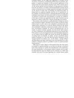
Figure 1-1 20 sequences of +2, -1.
This divisor we will call by its variable name f. Thus, whether con-
sciously or subconsciously, on any given trade you are selecting a value
for f when you decide how many contracts or shares to put on.
Refer now to Figure 1-1. This represents a game where you have a
50% chance of winning $2 versus a 50% chance of losing $1 on every
play. Notice that here the optimal f is .25 when the TWR is 10.55 after
40 bets (20 sequences of +2, -1). TWR stands for Terminal Wealth Rel-
ative. It represents the return on your stake as a multiple. A TWR of
10.55 means you would have made 10.55 times your original stake, or
955% profit. Now look at what happens if you bet only 15% away from
the optimal .25 f. At an f of .1 or .4 your TWR is 4.66. This is not even
half of what it is at .25, yet you are only 15% away from the optimal and
only 40 bets have elapsed!
How much are we talking about in terms of dollars? At f = .1, you
would be making 1 bet for every $10 in your stake. At f = .4, you would
be making I bet for every $2.50 in your stake. Both make the same
amount with a TWR of 4.66. At f = .25, you are making 1 bet for every
$4 in your stake. Notice that if you make 1 bet for every $4 in your
stake, you will make more than twice as much after 40 bets as you
would if you were making 1 bet for every $2.50 in your stake! Clearly it
does not pay to overbet. At 1 bet per every $2.50 in your stake you make
the same amount as if you had bet a quarter of that amount, 1 bet for ev-
ery $10 in your stake! Notice that in a 50/50 game where you win twice
the amount that you lose, at an f of .5 you are only breaking even! That
means you are only breaking even if you made 1 bet for every $2 in
your stake. At an f greater than .5 you are losing in this game, and it is
simply a matter of time until you are completely tapped out! In other
words, if your fin this 50/50, 2:1 game is .25 beyond what is optimal,
you will go broke with a probability that approaches certainty as you

continue to play. Our goal, then, is to objectively find the peak of the f
curve for a given trading system.
In this discussion certain concepts will be illuminated in terms of
gambling illustrations. The main difference between gambling and spec-
ulation is that gambling creates risk (and hence many people are op-
posed to it) whereas speculation is a transference of an already existing
risk (supposedly) from one party to another. The gambling illustrations
are used to illustrate the concepts as clearly and simply as possible. The
mathematics of money management and the principles involved in trad-
ing and gambling are quite similar. The main difference is that in the
math of gambling we are usually dealing with Bernoulli outcomes (only
two possible outcomes), whereas in trading we are dealing with the en-
tire probability distribution that the trade may take.
BASIC CONCEPTS
A probability statement is a number between 0 and 1 that specifies
how probable an outcome is, with 0 being no probability whatsoever of
the event in question occurring and 1 being that the event in question is
certain to occur. An independent trials process (sampling with replace-
ment) is a sequence of outcomes where the probability statement is con-
stant from one event to the next. A coin toss is an example of just such a
process. Each toss has a 50/50 probability regardless of the outcome of
the prior toss. Even if the last 5 flips of a coin were heads, the probabili-
ty of this flip being heads is unaffected and remains .5.
- 9 -
Naturally, the other type of random process is one in which the out-
come of prior events does affect the probability statement, and naturally,
the probability statement is not constant from one event to the next.
These types of events are called dependent trials processes (sampling
without replacement). Blackjack is an example of just such a process.
Once a card is played, the composition of the deck changes. Suppose a

new deck is shuffled and a card removed-say, the ace of diamonds. Prior
to removing this card the probability of drawing an ace was 4/52 or
.07692307692. Now that an ace has been drawn from the deck, and not
replaced, the probability of drawing an ace on the next draw is 3/51 or
.05882352941.
Try to think of the difference between independent and dependent
trials processes as simply whether the probability statement is fixed
(independent trials) or variable (dependent trials) from one event to
the next based on prior outcomes. This is in fact the only difference.
THE RUNS TEST
When we do sampling without replacement from a deck of cards,
we can determine by inspection that there is dependency. For certain
events (such as the profit and loss stream of a system's trades) where de-
pendency cannot be determined upon inspection, we have the runs test.
The runs test will tell us if our system has more (or fewer) streaks of
consecutive wins and losses than a random distribution.
The runs test is essentially a matter of obtaining the Z scores for the
win and loss streaks of a system's trades. A Z score is how many stan-
dard deviations you are away from the mean of a distribution. Thus, a Z
score of 2.00 is 2.00 standard deviations away from the mean (the ex-
pectation of a random distribution of streaks of wins and losses).
The Z score is simply the number of standard deviations the data is
from the mean of the Normal Probability Distribution. For example, a Z
score of 1.00 would mean that the data you arc testing is within 1 stan-
dard deviation from the mean. Incidentally, this is perfectly normal.
The Z score is then converted into a confidence limit, sometimes
also called a degree of certainty. The area under the curve of the Nor-
mal Probability Function at 1 standard deviation on either side of the
mean equals 68% of the total area under the curve. So we take our Z
score and convert it to a confidence limit, the relationship being that the

Z score is a number of standard deviations from the mean and the confi-
dence limit is the percentage of area under the curve occupied at so
many standard deviations.
Confidence Limit (%) Z Score
99.73 3.00
99 2.58
98 2.33
97 2.17
96 2.05
95.45 2.00
95 1.96
90 1.64
With a minimum of 30 closed trades we can now compute our Z
scores. What we are trying to answer is how many streaks of wins (loss-
es) can we expect from a given system? Are the win (loss) streaks of the
system we are testing in line with what we could expect? If not, is there
a high enough confidence limit that we can assume dependency exists
between trades -i.e., is the outcome of a trade dependent on the outcome
of previous trades?
Here then is the equation for the runs test, the system's Z score:
(1.01) Z = (N*(R 5)-X)/((X*(X-N))/(N-1))^(1/2)
where
N = The total number of trades in the sequence.
R = The total number of runs in the sequence.
X = 2*W*L
W = The total number of winning trades in the sequence.
L = The total number of losing trades in the sequence.
Here is how to perform this computation:
1. Compile the following data from your run of trades:
A. The total number of trades, hereafter called N.

B. The total number of winning trades and the total number of losing
trades. Now compute what we will call X. X = 2*Total Number of
Wins*Total Number of Losses.
C. The total number of runs in a sequence. We'll call this R.
2. Let's construct an example to follow along with. Assume the fol-
lowing trades:
-3 +2 +7 -4 +1 -1 +1 +6 -1 0 -2 +1
The net profit is +7. The total number of trades is 12, so N = 12, to
keep the example simple. We are not now concerned with how big the
wins and losses are, but rather how many wins and losses there are and
how many streaks. Therefore, we can reduce our run of trades to a sim-
ple sequence of pluses and minuses. Note that a trade with a P&L of 0 is
regarded as a loss. We now have:
- + + - + - + + - - - +
As can be seen, there are 6 profits and 6 losses; therefore, X =
2*6*6 = 72. As can also be seen, there are 8 runs in this sequence; there-
fore, R = 8. We define a run as anytime you encounter a sign change
when reading the sequence as just shown from left to right (i.e.,
chronologically). Assume also that you start at 1.
1. You would thus count this sequence as follows:
- + + - + - + + - - - +
1 2 3 4 5 6 7 8
2. Solve the expression:
N*(R 5)-X
For our example this would be:
12*(8-5)-72
12*7.5-72
90-72
18
3. Solve the expression:

(X*(X-N))/(N-1)
For our example this would be:
(72*(72-12))/(12-1)
(72*60)/11
4320/11
392.727272
4. Take the square root of the answer in number 3. For our example
this would be:
392.727272^(l/2) = 19.81734777
5. Divide the answer in number 2 by the answer in number 4. This is
your Z score. For our example this would be:
18/19.81734777 = .9082951063
6. Now convert your Z score to a confidence limit. The distribution of
runs is binomially distributed. However, when there are 30 or more
trades involved, we can use the Normal Distribution to very closely
approximate the binomial probabilities. Thus, if you are using 30 or
more trades, you can simply convert your Z score to a confidence
limit based upon Equation (3.22) for 2-tailed probabilities in the
Normal Distribution.
The runs test will tell you if your sequence of wins and losses con-
tains more or fewer streaks (of wins or losses) than would ordinarily be
expected in a truly random sequence, one that has no dependence be-
tween trials. Since we are at such a relatively low confidence limit in
our example, we can assume that there is no dependence between trials
in this particular sequence.
If your Z score is negative, simply convert it to positive (take the
absolute value) when finding your confidence limit. A negative Z score
implies positive dependency, meaning fewer streaks than the Normal
Probability Function would imply and hence that wins beget wins and
losses beget losses. A positive Z score implies negative dependency,

meaning more streaks than the Normal Probability Function would im-
ply and hence that wins beget losses and losses beget wins.
What would an acceptable confidence limit be? Statisticians gener-
ally recommend selecting a confidence limit at least in the high nineties.
Some statisticians recommend a confidence limit in excess of 99% in or-
der to assume dependency, some recommend a less stringent minimum
of 95.45% (2 standard deviations).
Rarely, if ever, will you find a system that shows confidence limits
in excess of 95.45%. Most frequently the confidence limits encountered
are less than 90%. Even if you find a system with a confidence limit be-
tween 90 and 95.45%, this is not exactly a nugget of gold. To assume
that there is dependency involved that can be capitalized upon to make a
substantial difference, you really need to exceed 95.45% as a bare mini-
mum.
- 10 -
As long as the dependency is at an acceptable confidence limit, you
can alter your behavior accordingly to make better trading decisions,
even though you do not understand the underlying cause of the depen-
dency. If you could know the cause, you could then better estimate
when the dependency was in effect and when it was not, as well as when
a change in the degree of dependency could be expected.
So far, we have only looked at dependency from the point of view
of whether the last trade was a winner or a loser. We are trying to deter-
mine if the sequence of wins and losses exhibits dependency or not. The
runs test for dependency automatically takes the percentage of wins and
losses into account. However, in performing the runs test on runs of
wins and losses, we have accounted for the sequence of wins and losses
but not their size. In order to have true independence, not only must the
sequence of the wins and losses be independent, the sizes of the wins
and losses within the sequence must also be independent. It is possible

for the wins and losses to be independent, yet their sizes to be dependent
(or vice versa). One possible solution is to run the runs test on only the
winning trades, segregating the runs in some way (such as those that are
greater than the median win and those that are less), and then look for
dependency among the size of the winning trades. Then do this for the
losing trades.
SERIAL CORRELATION
There is a different, perhaps better, way to quantify this possible de-
pendency between the size of the wins and losses. The technique to be
discussed next looks at the sizes of wins and losses from an entirely dif-
ferent perspective mathematically than the does runs test, and hence,
when used in conjunction with the runs test, measures the relationship of
trades with more depth than the runs test alone could provide. This tech-
nique utilizes the linear correlation coefficient, r, sometimes called
Pearson's r, to quantify the dependency/independency relationship.
Now look at Figure 1-2. It depicts two sequences that are perfectly
correlated with each other. We call this effect positive correlation.
Figure 1-2 Positive correlation (r = +1.00).
Figure 1-3 Negative correlation (r = -1 .00).
Now look at Figure 1-3. It shows two sequences that are perfectly
negatively correlated with each other. When one line is zigging the other
is zagging. We call this effect negative correlation.
The formula for finding the linear correlation coefficient, r, between
two sequences, X and Y, is as follows (a bar over a variable means the
arithmetic mean of the variable):
(1.02) R = (∑
a
(X
a
-X[])*(Y

a
-Y[]))/((∑
a
(X
a
-X[])^2)^(1/2)*(∑
a
(Y
a
-
Y[])^2)^(l/2))
Here is how to perform the calculation:
7. Average the X's and the Y's (shown as X[] and Y[]).
8. For each period find the difference between each X and the average
X and each Y and the average Y.
9. Now calculate the numerator. To do this, for each period multiply
the answers from step 2-in other words, for each period multiply
together the differences between that period's X and the average X
and between that period's Y and the average Y.
10. Total up all of the answers to step 3 for all of the periods. This is
the numerator.
11. Now find the denominator. To do this, take the answers to step 2
for each period, for both the X differences and the Y differences,
and square them (they will now all be positive numbers).
12. Sum up the squared X differences for all periods into one final to-
tal. Do the same with the squared Y differences.
13. Take the square root to the sum of the squared X differences you
just found in step 6. Now do the same with the Y's by taking the
square root of the sum of the squared Y differences.
14. Multiply together the two answers you just found in step 1 - that is,

multiply together the square root of the sum of the squared X dif-
ferences by the square root of the sum of the squared Y differences.
This product is your denominator.
15. Divide the numerator you found in step 4 by the denominator you
found in step 8. This is your linear correlation coefficient, r.
The value for r will always be between +1.00 and -1.00. A value of
0 indicates no correlation whatsoever.
Now look at Figure 1-4. It represents the following sequence of 21
trades:
1, 2, 1, -1, 3, 2, -1, -2, -3, 1, -2, 3, 1, 1, 2, 3, 3, -1, 2, -1, 3
4
2
0
-2
-4
Figure 1-4 Individual outcomes of 21 trades.
We can use the linear correlation coefficient in the following man-
ner to see if there is any correlation between the previous trade and the
current trade. The idea here is to treat the trade P&L's as the X values in
the formula for r. Superimposed over that we duplicate the same trade
P&L's, only this time we skew them by 1 trade and use these as the Y
values in the formula for r. In other words, the Y value is the previous X
value. (See Figure 1-5.).
4
2
0
-2
-4
Figure 1-5 Individual outcomes of 21 trades skewed by 1 trade.
A(X) B(X) C(X-X[]) D(Y-Y[]) E(C*D) F(C^2) G(D^2)

1
2 1 1.2 0.3 0.36 1.44 0.09
1 2 0.2 1.3 0.26 0.04 1.69
-1 1 -1.8 0.3 -0.54 3.24 0.09
- 11 -
3 -1 2.2 -1.7 -3.74 4.84 2.89
2 3 1.2 2.3 2.76 1.44 5.29
-1 2 -1.8 1.3 -2.34 3.24 1.69
-2 -1 -2.8 -1.7 4.76 7.84 2.89
-3 -2 -3.8 -2.7 10.26 14.44 7.29
1 -3 0.2 -3.7 -0.74 0.04 13.69
-2 1 -2.8 0.3 -0.84 7.84 0.09
3 -2 2.2 -2.7 -5.94 4.84 7.29
1 3 0.2 2.3 0.46 0.04 5.29
1 1 0.2 0.3 0.06 0.04 0.09
2 1 1.2 0.3 0.36 1.44 0.09
3 2 2.2 1.3 2.86 4.84 1.69
3 3 2.2 2.3 5.06 4.84 5.29
-1 3 -1.8 2.3 -4.14 3.24 5.29
2 -1 1.2 -1.7 -2.04 1.44 2.89
-1 2 -1.8 1.3 -2.34 3.24 1.69
3 -1 2.2 -1.7 -3.74 4.84 2.89
3
X[] = .8 Y[] = .7 Totals 0.8 73.2 68.2
The averages differ because you only average those X's and Y's that
have a corresponding X or Y value (i.e., you average only those values
that overlap), so the last Y value (3) is not figured in the Y average nor
is the first X value (1) figured in the x average.
The numerator is the total of all entries in column E (0.8). To find
the denominator, we take the square root of the total in column F,

which is 8.555699, and we take the square root to the total in column
G, which is 8.258329, and multiply them together to obtain a denomina-
tor of 70.65578. We now divide our numerator of 0.8 by our denomina-
tor of 70.65578 to obtain .011322. This is our linear correlation coeffi-
cient, r.
The linear correlation coefficient of .011322 in this case is hardly
indicative of anything, but it is pretty much in the range you can expect
for most trading systems. High positive correlation (at least .25) gener-
ally suggests that big wins are seldom followed by big losses and vice
versa. Negative correlation readings (below 25 to 30) imply that big
losses tend to be followed by big wins and vice versa. The correlation
coefficients can be translated, by a technique known as Fisher's Z
transformation, into a confidence level for a given number of trades.
This topic is treated in Appendix C.
Negative correlation is just as helpful as positive correlation. For ex-
ample, if there appears to be negative correlation and the system has just
suffered a large loss, we can expect a large win and would therefore
have more contracts on than we ordinarily would. If this trade proves to
be a loss, it will most likely not be a large loss (due to the negative cor-
relation).
Finally, in determining dependency you should also consider out-of-
sample tests. That is, break your data segment into two or more parts. If
you see dependency in the first part, then see if that dependency also ex-
ists in the second part, and so on. This will help eliminate cases where
there appears to be dependency when in fact no dependency exists.
Using these two tools (the runs test and the linear correlation coeffi-
cient) can help answer many of these questions. However, they can only
answer them if you have a high enough confidence limit and/or a high
enough correlation coefficient. Most of the time these tools are of little
help, because all too often the universe of futures system trades is domi-

nated by independency. If you get readings indicating dependency, and
you want to take advantage of it in your trading, you must go back and
incorporate a rule in your trading logic to exploit the dependency. In
other words, you must go back and change the trading system logic to
account for this dependency (i.e., by passing certain trades or breaking
up the system into two different systems, such as one for trades after
wins and one for trades after losses). Thus, we can state that if depen-
dency shows up in your trades, you haven't maximized your system. In
other words, dependency, if found, should be exploited (by changing the
rules of the system to take advantage of the dependency) until it no
longer appears to exist. The first stage in money management is there-
fore to exploit, and hence remove, any dependency in trades.
For more on dependency than was covered in Portfolio Manage-
ment Formulas and reiterated here, see Appendix C, "Further on De-
pendency: The Turning Points and Phase Length Tests."
We have been discussing dependency in the stream of trade profits
and losses. You can also look for dependency between an indicator and
the subsequent trade, or between any two variables. For more on these
concepts, the reader is referred to the section on statistical validation of
a trading system under "The Binomial Distribution" in Appendix B.
COMMON DEPENDENCY ERRORS
As traders we must generally assume that dependency does not exist
in the marketplace for the majority of market systems. That is, when
trading a given market system, we will usually be operating in an envi-
ronment where the outcome of the next trade is not predicated upon the
outcome(s) of prior trade(s). That is not to say that there is never depen-
dency between trades for some market systems (because for some mar-
ket systems dependency does exist), only that we should act as though
dependency does not exist unless there is very strong evidence to the
contrary. Such would be the case if the Z score and the linear correlation

coefficient indicated dependency, and the dependency held up across
markets and across optimizable parameter values. If we act as though
there is dependency when the evidence is not overwhelming, we may
well just be fooling ourselves and causing more self-inflicted harm than
good as a result. Even if a system showed dependency to a 95% confi-
dence limit for all values of a parameter, it still is hardly a high enough
confidence limit to assume that dependency does in fact exist between
the trades of a given market or system.
A type I error is committed when we reject an hypothesis that
should be accepted. If, however, we accept an hypothesis when it should
be rejected, we have committed a type II error. Absent knowledge of
whether an hypothesis is correct or not, we must decide on the penalties
associated with a type I and type II error. Sometimes one type of error is
more serious than the other, and in such cases we must decide whether
to accept or reject an unproven hypothesis based on the lesser penalty.
Suppose you are considering using a certain trading system, yet
you're not extremely sure that it will hold up when you go to trade it
real-time. Here, the hypothesis is that the trading system will hold up
real-time. You decide to accept the hypothesis and trade the system. If it
does not hold up, you will have committed a type II error, and you will
pay the penalty in terms of the losses you have incurred trading the sys-
tem real-time. On the other hand, if you choose to not trade the system,
and it is profitable, you will have committed a type I error. In this in-
stance, the penalty you pay is in forgone profits.
Which is the lesser penalty to pay? Clearly it is the latter, the for-
gone profits of not trading the system. Although from this example you
can conclude that if you're going to trade a system real-time it had better
be profitable, there is an ulterior motive for using this example. If we as-
sume there is dependency, when in fact there isn't, we will have commit-
ted a type 'II error. Again, the penalty we pay will not be in forgone

profits, but in actual losses. However, if we assume there is not depen-
dency when in fact there is, we will have committed a type I error and
our penalty will be in forgone profits. Clearly, we are better off paying
the penalty of forgone profits than undergoing actual losses. Therefore,
unless there is absolutely overwhelming evidence of dependency, you
are much better off assuming that the profits and losses in trading
(whether with a mechanical system or not) are independent of prior out-
comes.
There seems to be a paradox presented here. First, if there is depen-
dency in the trades, then the system is 'suboptimal. Yet dependency can
never be proven beyond a doubt. Now, if we assume and act as though
there is dependency (when in fact there isn't), we have committed a
more expensive error than if we assume and act as though dependency
does not exist (when in fact it does). For instance, suppose we have a
system with a history of 60 trades, and suppose we see dependency to a
confidence level of 95% based on the runs test. We want our system to
be optimal, so we adjust its rules accordingly to exploit this apparent de-
pendency. After we have done so, say we are left with 40 trades, and de-
pendency no longer is apparent. We are therefore satisfied that the sys-
tem rules are optimal. These 40 trades will now have a higher optimal f
than the entire 60 (more on optimal f later in this chapter).
If you go and trade this system with the new rules to exploit the de-
pendency, and the higher concomitant optimal f, and if the dependency
is not present, your performance will be closer to that of the 60 trades,
rather than the superior 40 trades. Thus, the f you have chosen will be
too far to the right, resulting in a big price to pay on your part for assum-
ing dependency. If dependency is there, then you will be closer to the
peak of the f curve by assuming that the dependency is there. Had you
decided not to assume it when in fact there was dependency, you would
- 12 -

tend to be to the left of the peak of the f curve, and hence your perfor-
mance would be suboptimal (but a lesser price to pay than being to the
right of the peak).
In a nutshell, look for dependency. If it shows to a high enough de-
gree across parameter values and markets for that system, then alter the
system rules to capitalize on the dependency. Otherwise, in the absence
of overwhelming statistical evidence of dependency, assume that it does
not exist, (thus opting to pay the lesser penalty if in fact dependency
does exist).
MATHEMATICAL EXPECTATION
By the same token, you are better off not to trade unless there is ab-
solutely overwhelming evidence that the market system you are contem-
plating trading will be profitable-that is, unless you fully expect the mar-
ket system in question to have a positive mathematical expectation when
you trade it realtime.
Mathematical expectation is the amount you expect to make or lose,
on average, each bet. In gambling parlance this is sometimes known as
the player's edge (if positive to the player) or the house's advantage (if
negative to the player):
(1.03) Mathematical Expectation = ∑[i = 1,N](P
i
*A
i
)
where
P = Probability of winning or losing.
A = Amount won or lost.
N = Number of possible outcomes.
The mathematical expectation is computed by multiplying each pos-
sible gain or loss by the probability of that gain or loss and then sum-

ming these products together.
Let's look at the mathematical expectation for a game where you
have a 50% chance of winning $2 and a 50% chance of losing $1 under
this formula:
Mathematical Expectation = (.5*2)+(.5*(-1)) = 1+(-5) = .5
In such an instance, of course, your mathematical expectation is to
win 50 cents per toss on average.
Consider betting on one number in roulette, where your mathemati-
cal expectation is:
ME = ((1/38)*35)+((37/38)*(-1))
= (.02631578947*35)+(.9736842105*(-1))
= (9210526315)+( 9736842105)
= 05263157903
Here, if you bet $1 on one number in roulette (American double-
zero) you would expect to lose, on average, 5.26 cents per roll. If you
bet $5, you would expect to lose, on average, 26.3 cents per roll. Notice
that different amounts bet have different mathematical expectations in
terms of amounts, but the expectation as a percentage of the amount
bet is always the same. The player's expectation for a series of bets is
the total of the expectations for the individual bets. So if you go play
$1 on a number in roulette, then $10 on a number, then $5 on a number,
your total expectation is:
ME = ( 0526*1)+( 0526*10)+( 0526*5) = 0526 526 .263 = 8416
You would therefore expect to lose, on average, 84.16 cents.
This principle explains why systems that try to change the sizes of
their bets relative to how many wins or losses have been seen (assuming
an independent trials process) are doomed to fail. The summation of
negative expectation bets is always a negative expectation!
The most fundamental point that you must understand in terms of
money management is that in a negative expectation game, there is no

money-management scheme that will make you a winner. If you con-
tinue to bet, regardless of how you manage your money, it is almost
certain that you will be a loser, losing your entire stake no matter how
large it was to start.
This axiom is not only true of a negative expectation game, it is true
of an even-money game as well. Therefore, the only game you have a
chance at winning in the long run is a positive arithmetic expectation
game. Then, you can only win if you either always bet the same constant
bet size or bet with an f value less than the f value corresponding to the
point where the geometric mean HPR is less than or equal to 1. (We will
cover the second part of this, regarding the geometric mean HPR, later
on in the text.)
This axiom is true only in the absence of an upper absorbing barrier.
For example, let's assume a gambler who starts out with a $100 stake
who will quit playing if his stake grows to $101. This upper target of
$101 is called an absorbing barrier. Let's suppose our gambler is always
betting $1 per play on red in roulette. Thus, he has a slight negative
mathematical expectation. The gambler is far more likely to see his
stake grow to $101 and quit than he is to see his stake go to zero and be
forced to quit. If, however, he repeats this process over and over, he will
find himself in a negative mathematical expectation. If he intends on
playing this game like this only once, then the axiom of going broke
with certainty, eventually, does not apply.
The difference between a negative expectation and a positive one is
the difference between life and death. It doesn't matter so much how
positive or how negative your expectation is; what matters is whether it
is positive or negative. So before money management can even be con-
sidered, you must have a positive expectancy game. If you don't, all the
money management in the world cannot save you
1

. On the other hand, if
you have a positive expectation, you can, through proper money man-
agement, turn it into an exponential growth function. It doesn't even
matter how marginally positive the expectation is!
In other words, it doesn't so much matter how profitable your trad-
ing system is on a 1 contract basis, so long as it is profitable, even if
only marginally so. If you have a system that makes $10 per contract per
trade (once commissions and slippage have been deducted), you can use
money management to make it be far more profitable than a system that
shows a $1,000 average trade (once commissions and slippage have
been deducted). What matters, then, is not how profitable your system
has been, but rather how certain is it that the system will show at least a
marginal profit in the future. Therefore, the most important preparation
a trader can do is to make as certain as possible that he has a positive
mathematical expectation in the future.
The key to ensuring that you have a positive mathematical expecta-
tion in the future is to not restrict your system's degrees of freedom. You
want to keep your system's degrees of freedom as high as possible to en-
sure the positive mathematical expectation in the future. This is accom-
plished not only by eliminating, or at least minimizing, the number of
optimizable parameters, but also by eliminating, or at least minimizing,
as many of the system rules as possible. Every parameter you add, every
rule you add, every little adjustment and qualification you add to your
system diminishes its degrees of freedom. Ideally, you will have a sys-
tem that is very primitive and simple, and that continually grinds out
marginal profits over time in almost all the different markets. Again, it
is important that you realize that it really doesn't matter how profitable
the system is, so long as it is profitable. The money you will make trad-
ing will be made by how effective the money management you employ
is. The trading system is simply a vehicle to give you a positive mathe-

matical expectation on which to use money management. Systems that
work (show at least a marginal profit) on only one or a few markets, or
have different rules or parameters for different markets, probably won't
work real-time for very long. The problem with most technically orient-
ed traders is that they spend too much time and effort hating the comput-
er crank out run after run of different rules and parameter values for
trading systems. This is the ultimate "woulda, shoulda, coulda" game. It
is completely counterproductive. Rather than concentrating your efforts
and computer time toward maximizing your trading system profits, di-
rect the energy toward maximizing the certainty level of a marginal
profit.
1
This rule is applicable to trading one market system only. When you
begin trading more than one market system, you step into a strange envi-
ronment where it is possible to include a market system with a negative
mathematical expectation as one of the markets being traded and actual-
ly have a higher net mathematical expectation than the net mathematical
expectation of the group before the inclusion of the negative expectation
system! Further, it is possible that the net mathematical expectation for
the group with the inclusion of the negative mathematical expectation
market system can be higher than the mathematical expectation of any
of the individual market systems! For the time being we will consider
only one market system at a time, so we most have a positive mathemat-
ical expectation in order for the money-management techniques to work.
- 13 -
TO REINVEST TRADING PROFITS OR NOT
Let's call the following system "System A." In it we have 2 trades:
the first making SO%, the second losing 40%. If we do not reinvest our
returns, we make 10%. If we do reinvest, the same sequence of trades
loses 10%.

System A
No Reinvestment With Reinvestment
Trade No. P&L Cumulative P&L Cumulative
100 100
1 50 150 50 150
2 -40 110 -60 90
Now let's look at System B, a gain of 15% and a loss of 5%, which
also nets out 10% over 2 trades on a nonreinvestment basis, just like
System A. But look at the results of System B with reinvestment: Unlike
system A, it makes money.
System B
No Reinvestment With Reinvestment
Trade No. P&L Cumulative P&L Cumulative
100 100
1 15 115 15 115
2 -5 110 -5.75 109.25
An important characteristic of trading with reinvestment that must
be realized is that reinvesting trading profits can turn a winning sys-
tem into a losing system but not vice versa! A winning system is turned
into a losing system in trading with reinvestment if the returns are not
consistent enough.
Changing the order or sequence of trades does not affect the final
outcome. This is not only true on a nonreinvestment basis, but also true
on a reinvestment basis (contrary to most people's misconception).
System A
No Reinvestment With Reinvestment
Trade No. P&L Cumulative P&L Cumulative
100 100
1 40 60 40 60
2 50 110 30 90

System B
No Reinvestment With Reinvestment
Trade No. P&L Cumulative P&L Cumulative
100 100
1 -5 95 -5 95
2 15 110 14.25 109.25
As can obviously be seen, the sequence of trades has no bearing on
the final outcome, whether viewed on a reinvestment or a nonreinvest-
ment basis. (One side benefit to trading on a reinvestment basis is that
the drawdowns tend to be buffered. As a system goes into and through a
drawdown period, each losing trade is followed by a trade with fewer
and fewer contracts.)
By inspection it would seem you are better off trading on a nonrein-
vestment basis than you are reinvesting because your probability of win-
ning is greater. However, this is not a valid assumption, because in the
real world we do not withdraw all of our profits and make up all of our
losses by depositing new cash into an account. Further, the nature of in-
vestment or trading is predicated upon the effects of compounding. If
we do away with compounding (as in the nonreinvestment basis), we
can plan on doing little better in the future than we can today, no matter
how successful our trading is between now and then. It is compounding
that takes the linear function of account growth and makes it a geomet-
ric function.
If a system is good enough, the profits generated on a reinvestment
basis will be far greater than those generated on a nonreinvestment ba-
sis, and that gap will widen as time goes by. If you have a system that
can beat the market, it doesn't make any sense to trade it in any other
way than to increase your amount wagered as your stake increases.
MEASURING A GOOD SYSTEM FOR REINVESTMENT
THE GEOMETRIC MEAN

So far we have seen how a system can be sabotaged by not being
consistent enough from trade to trade. Does this mean we should close
up and put our money in the bank?
Let's go back to System A, with its first 2 trades. For the sake of il-
lustration we are going to add two winners of 1 point each.
System A
No Reinvestment With Reinvestment
Trade No. P&L Cumulative P&L Cumulative
100 100
1 50 150 50 150
2 -40 110 -60 90
3 1 111 0.9 90.9
4 1 112 0.909 91.809
Percentage of Wins 75% 75%
Avg. Trade 3 - 2.04775
Risk/Rew. 1.3 0.86
Std. Dev. 31.88 39.00
Avg. Trade/Std. Dev. 0.09 -0.05
Now let's take System B and add 2 more losers of 1 point each.
System B
No Reinvestment With Reinvestment
Trade No. P&L Cumulative P&L Cumulative
100 100
1 15 115 15 115
2 - 5 110 -5.75 109.25
3 -1 109 -1.0925 108.1575
4 - 1 108 -1.08157 107.0759
Percentage of Wins 25% 25%
Avg. Trade 2 1.768981
Risk/Rew. 2.14 1.89

Std. Dev. 7.68 7.87
Avg. Trade/Std. Dev. 0.26 0.22
Now, if consistency is what we're really after, let's look at a bank
account, the perfectly consistent vehicle (relative to trading), paying 1
point per period. We'll call this series System C.
System C
No Reinvestment With Reinvestment
Trade No. P&L Cumulative P&L Cumulative
100 100
1 1 101 1 101
2 1 102 1.01 102.01
3 1 103 1.0201 103.0301
4 1 104 1.030301 104.0604
Percentage of Wins 1.00 1 .00
Avg. Trade 1 1.015100
Risk/Rew. Infinite Infinite
Std. Dev. 0.00 0.01
Avg. Trade/Std. Dev. Infinite 89.89
Our aim is to maximize our profits under reinvestment trading. With
that as the goal, we can see that our best reinvestment sequence comes
from System B. How could we have known that, given only information
regarding nonreinvestment trading? By percentage of winning trades?
By total dollars? By average trade? The answer to these questions is
"no," because answering "yes" would have us trading System A (but this
is the solution most futures traders opt for). What if we opted for most
consistency (i.e., highest ratio average trade/standard deviation or lowest
standard deviation)? How about highest risk/reward or lowest draw-
down? These are not the answers either. If they were, we should put our
money in the bank and forget about trading.
System B has the tight mix of profitability and consistency. Systems

A and C do not. That is why System B performs the best under reinvest-
ment trading. What is the best way to measure this "right mix"? It turns
out there is a formula that will do just that-the geometric mean. This is
simply the Nth root of the Terminal Wealth Relative (TWR), where N is
the number of periods (trades). The TWR is simply what we've been
computing when we figure what the final cumulative amount is under
reinvestment, In other words, the TWRs for the three systems we just
saw are:
System TWR
System A .91809
System B 1.070759
System C 1.040604
Since there are 4 trades in each of these, we take the TWRs to the
4th root to obtain the geometric mean:
System Geometric Mean
System A 0. 978861
System B 1.017238
System C 1.009999
(1.04) TWR = ∏[i = 1,N]HPR
i
(1.05) Geometric Mean = TWR^(1/N)
- 14 -
where
N = Total number of trades.
HPR = Holding period returns (equal to 1 plus the rate of return -e
.g., an HPR of 1.10 means a 10% return over a given period, bet, or
trade).
TWR = The number of dollars of value at the end of a run of peri-
ods/bets/trades per dollar of initial investment, assuming gains and loss-
es are allowed to compound.

Here is another way of expressing these variables:
(1.06) TWR = Final Stake/Starting Stake
The geometric mean (G) equals your growth factor per play, or:
(1.07) G = (Final Stake/Starting Stake)^(I/Number of Plays)
Think of the geometric mean as the "growth factor per play" of your
stake. The system or market with the highest geometric mean is the sys-
tem or market that makes the most profit trading on a reinvestment of
returns basis. A geometric mean less than one means that the system
would have lost money if you were trading it on a reinvestment basis.
Investment performance is often measured with respect to the dis-
persion of returns. Measures such as the Sharpe ratio, Treynor measure,
Jensen measure, Vami, and so on, attempt to relate investment perfor-
mance to dispersion. The geometric mean here can be considered anoth-
er of these types of measures. However, unlike the other measures, the
geometric mean measures investment performance relative to dispersion
in the same mathematical form as that in which the equity in your ac-
count is affected.
Equation (1.04) bears out another point. If you suffer an HPR of 0,
you will be completely wiped out, because anything multiplied by zero
equals zero. Any big losing trade will have a very adverse effect on the
TWR, since it is a multiplicative rather than additive function. Thus we
can state that in trading you are only as smart as your dumbest mis-
take.
HOW BEST TO REINVEST
Thus far we have discussed reinvestment of returns in trading
whereby we reinvest 100% of our stake on all occasions. Although we
know that in order to maximize a potentially profitable situation we
must use reinvestment, a 100% reinvestment is rarely the wisest thing to
do.
Take the case of a fair bet (50/50) on a coin toss. Someone is will-

ing to pay you $2 if you win the toss but will charge you $1 if you lose.
Our mathematical expectation is .5. In other words, you would expect to
make 50 cents per toss, on average. This is true of the first toss and all
subsequent tosses, provided you do not step up the amount you are wa-
gering. But in an independent trials process this is exactly what you
should do. As you win you should commit more and more to each toss.
Suppose you begin with an initial stake of one dollar. Now suppose
you win the first toss and are paid two dollars. Since you had your entire
stake ($1) riding on the last bet, you bet your entire stake (now $3) on
the next toss as well. However, this next toss is a loser and your entire
$3 stake is gone. You have lost your original $1 plus the $2 you had
won. If you had won the last toss, it would have paid you $6 since you
had three $1 bets on it. The point is that if you are betting 100% of your
stake, you'll be wiped out as soon as you encounter a losing wager, an
inevitable event. If we were to replay the previous scenario and you had
bet on a nonreinvestment basis (i.e., constant bet size) you would have
made $2 on the first bet and lost $1 on the second. You would now be
net ahead $1 and have a total stake of $2.
Somewhere between these two scenarios lies the optimal betting ap-
proach for a positive expectation. However, we should first discuss the
optimal betting strategy for a negative expectation game. When you
know that the game you are playing has a negative mathematical expec-
tation, the best bet is no bet. Remember, there is no money-management
strategy that can turn a losing game into a winner. 'However, if you
must bet on a negative expectation game, the next best strategy is the
maximum boldness strategy. In other words, you want to bet on as few
trials as possible (as opposed to a positive expectation game, where you
want to bet on as many trials as possible). The more trials, the greater
the likelihood that the positive expectation will be realized, and hence
the greater the likelihood that betting on the negative expectation side

will lose. Therefore, the negative expectation side has a lesser and lesser
chance of losing as the length of the game is shortened - i.e., as the num-
ber of trials approaches 1. If you play a game whereby you have a 49%
chance of winning $1 and a 51% of losing $1, you are best off betting
on only 1 trial. The more trials you bet on, the greater the likelihood you
will lose, with the probability of losing approaching certainty as the
length of the game approaches infinity. That isn't to say that you are in a
positive expectation for the 1 trial, but you have at least minimized the
probabilities of being a loser by only playing 1 trial.
Return now to a positive expectation game. We determined at the
outset of this discussion that on any given trade, the quantity that a trad-
er puts on can be expressed as a factor, f, between 0 and 1, that repre-
sents the trader's quantity with respect to both the perceived loss on the
next trade and the trader's total equity. If you know you have an edge
over N bets but you do not know which of those N bets will be winners
(and for how much), and which will be losers (and for how much), you
are best off (in the long run) treating each bet exactly the same in terms
of what percentage of your total stake is at risk. This method of always
trading a fixed fraction of your stake has shown time and again to be the
best staking system. If there is dependency in your trades, where win-
ners beget winners and losers beget losers, or vice versa, you are still
best off betting a fraction of your total stake on each bet, but that frac-
tion is no longer fixed. In such a case, the fraction must reflect the effect
of this dependency (that is, if you have not yet "flushed" the dependency
out of your system by creating system rules to exploit it).
"Wait," you say. "Aren't staking systems foolish to begin with?
Haven't we seen that they don't overcome the house advantage, they
only increase our total action?" This is absolutely true for a situation
with a negative mathematical expectation. For a positive mathematical
expectation, it is a different story altogether. In a positive expectancy

situation the trader/gambler is faced with the question of how best to ex-
ploit the positive expectation.
OPTIMAL FIXED FRACTIONAL TRADING
We have spent the course of this discussion laying the groundwork
for this section. We have seen that in order to consider betting or trading
a given situation or system you must first determine if a positive mathe-
matical expectation exists. We have seen that what is seemingly a "good
bet" on a mathematical expectation basis (i.e., the mathematical expecta-
tion is positive) may in fact not be such a good bet when you consider
reinvestment of returns, if you are reinvesting too high a percentage of
your winnings relative to the dispersion of outcomes of the system.
Reinvesting returns never raises the mathematical expectation (as a per-
centage-although it can raise the mathematical expectation in terms of
dollars, which it does geometrically, which is why we want to reinvest).
If there is in fact a positive mathematical expectation, however small,
the next step is to exploit this positive expectation to its fullest potential.
For an independent trials process, this is achieved by reinvesting a fixed
fraction of your total stake.
2
And how do we find this optimal f? Much work has been done in re-
cent decades on this topic in the gambling community, the most famous
and accurate of which is known as the Kelly Betting System. This is ac-
tually an application of a mathematical idea developed in early 1956 by
John L. Kelly, Jr.
3
The Kelly criterion states that we should bet that
fixed fraction of our stake (f) which maximizes the growth function
G(f):
(1.08) G(f) = P*ln(l+B*f)+(1 -P)*ln(l-f)
where

f = The optimal fixed fraction.
P = The probability of a winning bet or trade.
B = The ratio of amount won on a winning bet to amount lost on a
losing bet.
ln() = The natural logarithm function.
2
For a dependent trials process, just as for an independent trials process, the idea
of betting a proportion of your total stake also yields the greatest exploitation of a
positive mathematical expectation. However, in a dependent trials process you
optimally bet a variable fraction of your total stake, the exact fraction for each in-
dividual bet being determined by the probabilities and payoffs involved for each
individual bet. This is analogous to trading a dependent trials process as two sep-
arate market systems.
3
Kelly, J. L., Jr., A New Interpretation of Information Rate, Bell System
Technical Journal, pp. 917-926, July, 1956.
- 15 -
As it turns out, for an event with two possible outcomes, this opti-
mal f
4
can be found quite easily with the Kelly formulas.
KELLY FORMULAS
Beginning around the late 1940s, Bell System engineers were work-
ing on the problem of data transmission over long-distance lines. The
problem facing them was that the lines were subject to seemingly ran-
dom, unavoidable "noise" that would interfere with the transmission.
Some rather ingenious solutions were proposed by engineers at Bell
Labs. Oddly enough, there are great similarities between this data com-
munications problem and the problem of geometric growth as pertains
to gambling money management (as both problems are the product of an

environment of favorable uncertainty). One of the outgrowths of these
solutions is the first Kelly formula. The first equation here is:
(1.09a) f = 2*P-l
or
(1.09b) f = P-Q
where
f = The optimal fixed fraction.
P = The probability of a winning bet or trade.
Q = The probability of a loss, (or the complement of P, equal to 1-
P).
Both forms of Equation (1.09) are equivalent.
Equation (l.09a) or (1.09b) will yield the correct answer for optimal
f provided the quantities are the same for both wins and losses. As an
example, consider the following stream of bets:
-1, +1, +1,-1,-1, +1, +1, +1, +1,-1
There are 10 bets, 6 winners, hence:
f = (.6*2)-l = 1.2-1 = .2
If the winners and losers were not all the same size, then this formu-
la would not yield the correct answer. Such a case would be our two-to-
one coin-toss example, where all of the winners were for 2 units and all
of the losers for 1 unit. For this situation the Kelly formula is:
(1.10a) f = ((B+1)*P-1)/B
where
f = The optimal fixed fraction.
P = The probability of a winning bet or trade.
B = The ratio of amount won on a winning bet to amount lost on a
losing bet.
In our two-to-one coin-toss example:
f = ((2+ l).5-l)/2
= (3*.5-l)/2

= (1.5 -l)/2
= .5/2
= .25
This formula will yield the correct answer for optimal f provided all
wins are always for the same amount and all losses are always for the
same amount. If this is not so, then this formula will not yield the cor-
rect answer.
The Kelly formulas are applicable only to outcomes that have a
Bernoulli distribution. A Bernoulli distribution is a distribution with
two possible, discrete outcomes. Gambling games very often have a
Bernoulli distribution. The two outcomes are how much you make when
you win, and how much you lose when you lose. Trading, unfortunately,
is not this simple. To apply the Kelly formulas to a non-Bernoulli distri-
bution of outcomes (such as trading) is a mistake. The result will not be
the true optimal f. For more on the Bernoulli distribution, consult Ap-
pendix B. Consider the following sequence of bets/trades:
+9, +18, +7, +1, +10, -5, -3, -17, -7
Since this is not a Bernoulli distribution (the wins and losses are of
different amounts), the Kelly formula is not applicable. However, let's
try it anyway and see what we get.
Since 5 of the 9 events are profitable, then P = .555. Now let's take
averages of the wins and losses to calculate B (here is where so many
4
As used throughout the text, f is always lowercase and in roman type. It is not to
be confused with the universal constant, F, equal to 4.669201609…, pertaining to
bifurcations in chaotic systems.
traders go wrong). The average win is 9, and the average loss is 8.
Therefore we say that B = 1.125. Plugging in the values we obtain:
f = ((1.125+1) .555-1)/1.125
= (2.125*.555-1)/1.125

= (1.179375-1)/1.125
= .179375/1.125
= .159444444
So we say f = .16. You will see later in this chapter that this is not
the optimal f. The optimal f for this sequence of trades is .24. Applying
the Kelly formula when all wins are not for the same amount and/or all
losses are not for the same amount is a mistake, for it will not yield the
optimal f.
Notice that the numerator in this formula equals the mathematical
expectation for an event with two possible outcomes as defined earlier.
Therefore, we can say that as long as all wins are for the same amount
and all losses are for the same amount (whether or not the amount that
can be won equals the amount that can be lost), the optimal f is:
(1.10b) f = Mathematical Expectation/B
where
f = The optimal fixed fraction.
B = The ratio of amount won on a winning bet to amount lost on a
losing bet.
The mathematical expectation is defined in Equation (1.03), but
since we must have a Bernoulli distribution of outcomes we must make
certain in using Equation (1.10b) that we only have two possible out-
comes.
Equation (l.l0a) is the most commonly seen of the forms of Equa-
tion (1.10) (which are all equivalent). However, the formula can be re-
duced to the following simpler form:
(1.10c) f = P-Q/B
where
f = The optimal fixed fraction.
P = The probability of a winning bet or trade.
Q = The probability of a loss (or the complement of P, equal to 1-P).

FINDING THE OPTIMAL F BY THE GEOMETRIC MEAN
In trading we can count on our wins being for varying amounts and
our losses being for varying amounts. Therefore the Kelly formulas
could not give us the correct optimal f. How then can we find our opti-
mal f to know how many contracts to have on and have it be mathemati-
cally correct?
Here is the solution. To begin with, we must amend our formula for
finding HPRs to incorporate f:
(1.11) HPR = 1+f*(-Trade/Biggest Loss)
where
f = The value we are using for f.
-Trade = The profit or loss on a trade (with the sign reversed so that
losses are positive numbers and profits are negative).
Biggest Loss = The P&L that resulted in the biggest loss. (This
should always be a negative number.)
And again, TWR is simply the geometric product of the HPRs and
geometric mean (G) is simply the Nth root of the TWR.
(1.12) TWR = ∏[i = 1,N](1+f*(-Trade
i
/Biggest Loss))
(1.13) G = (∏[i = 1,N](1+f*(-Trade
i
/Biggest Loss))]^(1/N)
where
f = The value we are using for f.
-Trade
i
= The profit or loss on the ith trade (with the sign reversed
so that losses are positive numbers and profits are negative).
Biggest Loss = The P&L that resulted in the biggest loss. (This

should always be a negative number.)
N = The total number of trades.
G = The geometric mean of the HPRs.
By looping through all values for I between .01 and 1, we can find
that value for f which results in the highest TWR. This is the value for
f that would provide us with the maximum return on our money using
fixed fraction. We can also state that the optimal f is the f that yields the
- 16 -
highest geometric mean. It matters not whether we look for highest
TWR or geometric mean, as both are maximized at the same value for f.
Doing this with a computer is easy, since both the TWR curve and
the geometric mean curve are smooth with only one peak. You simply
loop from f = .01 to f = 1.0 by .01. As soon as you get a TWR that is
less than the previous TWR, you know that the f corresponding to the
previous TWR is the optimal f. You can employ many other search al-
gorithms to facilitate this process of finding the optimal f in the range of
0 to 1. One of the fastest ways is with the parabolic interpolation search
procedure detailed in portfolio Management Formulas.
TO SUMMARIZE THUS FAR
You have seen that a good system is the one with the highest geo-
metric mean. Yet to find the geometric mean you must know f. You
may find this confusing. Here now is a summary and clarification of the
process:
Take the trade listing of a given market system.
1. Find the optimal f, either by testing various f values from 0 to 1 or
through iteration. The optimal f is that which yields the highest
TWR.
2. Once you have found f, you can take the Nth root of the TWR that
corresponds to your f, where N is the total number of trades. This is
your geometric mean for this market system. You can now use this

geometric mean to make apples-to-apples comparisons with other
market systems, as well as use the f to know how many contracts to
trade for that particular market system.
Once the highest f is found, it can readily be turned into a dollar
amount by dividing the biggest loss by the negative optimal f. For ex-
ample, if our biggest loss is $100 and our optimal f is .25, then -$100/-
.25 = $400. In other words, we should bet 1 unit for every $400 we have
in our stake.
If you're having trouble with some of these concepts, try thinking in
terms of betting in units, not dollars (e.g., one $5 chip or one futures
contract or one 100-share unit of stock). The number of dollars you allo-
cate to each unit is calculated by figuring your largest loss divided by
the negative optimal f.
The optimal f is a result of the balance between a system's profit-
making ability (on a constant 1-unit basis) and its risk (on a constant 1-
unit basis).
Most people think that the optimal fixed fraction is that percentage
of your total stake to bet, This is absolutely false. There is an interim
step involved. Optimal f is not in itself the percentage of your total stake
to bet, it is the divisor of your biggest loss. The quotient of this division
is what you divide your total stake by to know how many bets to make
or contracts to have on.
You will also notice that margin has nothing whatsoever to do
with what is the mathematically optimal number of contracts to have
on. Margin doesn't matter because the sizes of individual profits and
losses are not the product of the amount of money put up as margin
(they would be the same whatever the size of the margin). Rather, the
profits and losses are the product of the exposure of 1 unit (1 futures
contract). The amount put up as margin is further made meaningless in a
money-management sense, because the size of the loss is not limited to

the margin.
Most people incorrectly believe that f is a straight-line function ris-
ing up and to the right. They believe this because they think it would
mean that the more you are willing to risk the more you stand to make.
People reason this way because they think that a positive mathematical
expectancy is just the mirror image of a negative expectancy. They mis-
takenly believe that if increasing your total action in a negative ex-
pectancy game results in losing faster, then increasing your total action
in a positive expectancy game will result in winning faster. This is not
true. At some point in a positive expectancy situation, further increasing
your total action works against you. That point is a function of both the
system's profitability and its consistency (i.e., its geometric mean), since
you are reinvesting the returns back into the system.
It is a mathematical fact that when two people face the same se-
quence of favorable betting or trading opportunities, if one uses the opti-
mal f and the other uses any different money-management system, then
the ratio of the optimal f bettor's stake to the other person's stake will in-
crease as time goes on, with higher and higher probability. In the long
run, the optimal f bettor will have infinitely greater wealth than any oth-
er money-management system bettor with a probability approaching 1.
Furthermore, if a bettor has the goal of reaching a specified fortune and
is facing a series of favorable betting or trading opportunities, the ex-
pected time to reach the fortune will be lower (faster) with optimal f
than with any other betting system.
Let's go back and reconsider the following sequence of bets (trades):
+9, +18, +7, +1, +10, -5, -3, -17, -7
Recall that we determined earlier in this chapter that the Kelly for-
mula was not applicable to this sequence, because the wins were not all
for the same amount and neither were the losses. We also decided to av-
erage the wins and average the losses and take these averages as our val-

ues into the Kelly formula (as many traders mistakenly do). Doing this
we arrived at an f value of .16. It was stated that this is an incorrect ap-
plication of Kelly, that it would not yield the optimal f. The Kelly for-
mula must be specific to a single bet. You cannot average your wins and
losses from trading and obtain the true optimal fusing the Kelly formula.
Our highest TWR on this sequence of bets (trades) is obtained at
.24, or betting $1 for every $71 in our stake. That is the optimal geomet-
ric growth you can squeeze out of this sequence of bets (trades) trading
fixed fraction. Let's look at the TWRs at different points along 100
loops through this sequence of bets. At 1 loop through (9 bets or trades),
the TWR for f = ,16 is 1.085, and for f = .24 it is 1.096. This means that
for 1 pass through this sequence of bets an f = .16 made 99% of what an
f = .24 would have made. To continue:
Passes
Throe
Total Bets
or Trades
TWR for
f=.24
TWR for
f=.16
Percentage
Difference
1 9 1.096 1.085 1
10 90 2.494 2.261 9.4
40 360 38.694 26.132 32.5
100 900 9313.312 3490.761 62.5
As can be seen, using an f value that we mistakenly figured from
Kelly only made 37.5% as much as did our optimal f of .24 after 900
bets or trades (100 cycles through the series of 9 outcomes). In other

words, our optimal f of .24, which is only .08 different from .16 (50%
beyond the optimal) made almost 267% the profit that f = .16 did after
900 bets!
Let's go another 11 cycles through this sequence of trades, so that
we now have a total of 999 trades. Now our TWR for f = .16 is
8563.302 (not even what it was for f = .24 at 900 trades) and our TWR
for f = .24 is 25,451.045. At 999 trades f = .16 is only 33.6% off = .24,
or f = .24 is 297% off = .16!
As you see, using the optimal f does not appear to offer much ad-
vantage over the short run, but over the long run it becomes more and
more important. The point is, you must give the program time when
trading at the optimal f and not expect miracles in the short run. The
more time (i.e., bets or trades) that elapses, the greater the difference
between using the optimal f and any other money-management strate-
gy.
GEOMETRIC AVERAGE TRADE
At this point the trader may be interested in figuring his or her geo-
metric average trade-that is, what is the average garnered per contract
per trade assuming profits are always reinvested and fractional contracts
can be purchased. This is the mathematical expectation when you are
trading on a fixed fractional basis. This figure shows you what effect
there is by losers occurring when you have many contracts on and
winners occurring when you have fewer contracts on. In effect, this
approximates how a system would have fared per contract per trade
doing fixed fraction. (Actually the geometric average trade is your
mathematical expectation in dollars per contract per trade. The geomet-
ric mean minus 1 is your mathematical expectation per trade-a geomet-
ric mean of 1.025 represents a mathematical expectation of 2.5% per
trade, irrespective of size.) Many traders look only at the average trade
of a market system to see if it is high enough to justify trading the sys-

tem. However, they should be looking at the geometric average trade
(GAT) in making their decision.
(1.14) GAT = G*(Biggest Loss/-f)
where
G = Geometric mean-1.
- 17 -
f = Optimal fixed fraction. (and, of course, our biggest loss is al-
ways a negative number).
For example, suppose a system has a geometric mean of 1.017238,
the biggest loss is $8,000, and the optimal f is .31. Our geometric aver-
age trade would be:
GAT = (1.017238-1)*(-$8,000/ 31)
= .017238*$25,806.45
= $444.85
WHY YOU MUST KNOW YOUR OPTIMAL F
The graph in Figure 1-6 further demonstrates the importance of us-
ing optimal fin fixed fractional trading. Recall our f curve for a 2:1 coin-
toss game, which was illustrated in Figure 1-1.
Let's increase the winning payout from 2 units to 5 units as is
demonstrated in Figure 1-6. Here your optimal f is .4, or to bet $1 for
every $2.50 in you stake. After 20 sequences of +5,-l (40 bets), your
$2.50 stake has grown to $127,482, thanks to optimal f. Now look what
happens in this extremely favorable situation if you miss the optimal f
by 20%. At f values of .6 and .2 you don't make a tenth as much as you
do at .4. This particular situation, a 50/50 bet paying 5 to 1, has a mathe-
matical expectation of (5*.5)+(1*( 5)) = 2, yet if you bet using an f val-
ue greater than .8 you lose money.
T
W
R

f values
0
20
40
60
80
100
120
0.05 0.15 0.25 0.35 0.45 0.55 0.65 0.75 0.85
140
Figure 1-6 20 sequences of +5, -1.
Two points must be illuminated here. The first is that whenever we
discuss a TWR, we assume that in arriving at that TWR we allowed
fractional contracts along the way. In other words, the TWR assumes
that you are able to trade 5.4789 contracts if that is called for at some
point. It is because the TWR calculation allows for fractional contracts
that the TWR will always be the same for a given set of trade outcomes
regardless of their sequence. You may argue that in real life this is not
the case. In real life you cannot trade fractional contracts. Your argu-
ment is correct. However, I am allowing the TWR to be calculated this
way because in so doing we represent the average TWR for all possible
starting stakes. If you require that all bets be for integer amounts, then
the amount of the starting stake becomes important. However, if you
were to average the TWRs from all possible starting stake
values using integer bets only, you would arrive at the same TWR
value that we calculate by allowing the fractional bet. Therefore, the
TWR value as calculated is more realistic than if we were to constrain it
to integer bets only, in that it is representative of the universe of out-
comes of different starting stakes.
Furthermore, the greater the equity in the account, the more trading

on an integer contract basis will be the same as trading on a fractional
contract basis. The limit here is an account with an infinite amount of
capital where the integer bet and fractional bet are for the same amounts
exactly.
This is interesting in that generally the closer you can stick to opti-
mal f, the better. That is to say that the greater the capitalization of an
account, the greater will be the effect of optimal f. Since optimal f will
make an account grow at the fastest possible rate, we can state that opti-
mal f will make itself work better and better for you at the fastest possi-
ble rate.
The graphs (Figures 1-1 and 1-6) bear out a few more interesting
points. The first is that at no other fixed fraction will you make more
money than you will at optimal f. In other words, it does not pay to bet
$1 for every $2 in your stake in the earlier example of a 5:1 game. In
such a case you would make more money if you bet $1 for every $2.50
in your stake. It does not pay to risk more than the optimal f-in fact,
you pay a price to do so!
Obviously, the greater the capitalization of an account the more ac-
curately you can stick to optimal f, as the dollars per single contract re-
quired are a smaller percentage of the total equity. For example, suppose
optimal f for a given market system dictates you trade 1 contract for ev-
ery $5,000 in an account. If an account starts out with $10,000 in equity,
it will need to gain (or lose) 50% before a quantity adjustment is neces-
sary. Contrast this to a $500,000 account, where there would be a con-
tract adjustment for every 1% change in equity. Clearly the larger ac-
count can better take advantage of the benefits provided by optimal f
than can the smaller account. Theoretically, optimal f assumes you can
trade in infinitely divisible quantities, which is not the case in real life,
where the smallest quantity you can trade in is a single contract. In the
asymptotic sense this does not matter. But in the real-life integer-bet

scenario, a good case could be presented for trading a market system
that requires as small a percentage of the account equity as possible, es-
pecially for smaller accounts. But there is a tradeoff here as well. Since
we are striving to trade in markets that would require us to trade in
greater multiples than other markets, we will be paying greater commis-
sions, execution costs, and slippage. Bear in mind that the amount re-
quired per contract in real life is the greater of the initial margin require-
ment and the dollar amount per contract dictated by the optimal f.
The finer you can cut it (i.e., the more frequently you can adjust the
size of the positions you are trading so as to align yourself with what the
optimal f dictates), the better off you are. Most accounts would therefore
be better off trading the smaller markets. Corn may not seem like a very
exciting market to you compared to the S&P's. Yet for most people the
corn market can get awfully exciting if they have a few hundred con-
tracts on.
Those who trade stocks or forwards (such as forex traders) have a
tremendous advantage here. Since you must calculate your optimal f
based on the outcomes (the P&Ls) on a 1-contract (1 unit) basis, you
must first decide what 1 unit is in stocks or forex. As a stock trader, say
you decide that I unit will be 100 shares. You will use the P&L stream
generated by trading 100 shares on each and every trade to determine
your optimal f. When you go to trade this particular stock (and let's say
your system calls for trading 2.39 contracts or units), you will be able to
trade the fractional part (the .39 part) by putting on 239 shares. Thus, by
being able to trade the fractional part of 1 unit, you are able to take more
advantage of optimal f. Likewise for forex traders, who must first decide
what 1 contract or unit is. For the forex trader, 1 unit may be one million
U.S. dollars or one million Swiss francs.
THE SEVERITY OF DRAWDOWN
It is important to note at this point that the drawdown you can ex-

pect with fixed fractional trading, as a percentage retracement of your
account equity, historically would have been at least as much as f per-
cent. In other words if f is .55, then your drawdown would have been at
least 55% of your equity (leaving you with 45% at one point). This is so
because if you are trading at the optimal f, as soon as your biggest loss
was hit, you would experience the drawdown equivalent to f. Again, as-
suming that f for a system is .55 and assuming that translates into trad-
ing 1 contract for every $10,000, this means that your biggest loss was
$5,500. As should by now be obvious, when the biggest loss was en-
countered (again we're speaking historically what would have
happened), you would have lost $5,500 for each contract you had on,
and would have had 1 contract on for every $10,000 in the account. At
that point, your drawdown is 55% of equity. Moreover, the drawdown
might continue: The next trade or series of trades might draw your ac-
count down even more. Therefore, the better a system, the higher the f.
The higher the f, generally the higher the drawdown, since the draw-
down (in terms of a percentage) can never be any less than the f as a
percentage. There is a paradox involved here in that if a system is good
enough to generate an optimal f that is a high percentage, then the draw-
down for such a good system will also be quite high. Whereas optimal
fallows you to experience the greatest geometric growth, it also gives
you enough rope to hang yourself with.
- 18 -
Most traders harbor great illusions about the severity of drawdowns.
Further, most people have fallacious ideas regarding the ratio of poten-
tial gains to dispersion of those gains.
We know that if we are using the optimal f when we are fixed frac-
tional trading, we can expect substantial drawdowns in terms of percent-
age equity retracements. Optimal f is like plutonium. It gives you a
tremendous amount of power, yet it is dreadfully dangerous. These sub-

stantial drawdowns are truly a problem, particularly for notices, in that
trading at the optimal f level gives them the chance to experience a cata-
clysmic loss sooner than they ordinarily might have. Diversification can
greatly buffer the drawdowns. This it does, but the reader is warned not
to expect to eliminate drawdown. In fact, the real benefit of diversifica-
tion is that it lets you get off many more trials, many more plays, in
the same time period, thus increasing your total profit. Diversification,
although usually the best means by which to buffer drawdowns, does
not necessarily reduce drawdowns, and in some instances, may actually
increase them!
Many people have the mistaken impression that drawdown can be
completely eliminated if they diversify effectively enough. To an extent
this is true, in that drawdowns can be buffered through effective diversi-
fication, but they can never be completely eliminated. Do not be delud-
ed. No matter how good the systems employed are, no matter how effec-
tively you diversify, you will still encounter substantial drawdowns. The
reason is that no matter of how uncorrelated your market systems are,
there comes a period when most or all of the market systems in your
portfolio zig in unison against you when they should be zagging. You
will have enormous difficulty finding a portfolio with at least 5 years of
historical data to it and all market systems employing the optimal f that
has had any less than a 30% drawdown in terms of equity retracement!
This is regardless of how many market systems you employ. If you want
to be in this and do it mathematically correctly, you better expect to be
nailed for 30% to 95% equity retracements. This takes enormous disci-
pline, and very few people can emotionally handle this.
When you dilute f, although you reduce the drawdowns arithmeti-
cally, you also reduce the returns geometrically. Why commit funds to
futures trading that aren't necessary simply to flatten out the equity
curve at the expense of your bottom-line profits? You can diversify

cheaply somewhere else.
Any time a trader deviates from always trading the same constant
contract size, he or she encounters the problem of what quantities to
trade in. This is so whether the trader recognizes this problem or not.
Constant contract trading is not the solution, as you can never experi-
ence geometric growth trading constant contract. So, like it or not, the
question of what quantity to take on the next trade is inevitable for ev-
eryone. To simply select an arbitrary quantity is a costly mistake. Opti-
mal f is factual; it is mathematically correct.
MODERN PORTFOLIO THEORY
Recall the paradox of the optimal f and a market system's draw-
down. The better a market system is, the higher the value for f. Yet the
drawdown (historically) if you are trading the optimal f can never be
lower than f. Generally speaking, then, the better the market system is,
the greater the drawdown will be as a percentage of account equity if
you are trading optimal f. That is, if you want to have the greatest geo-
metric growth in an account, then you can count on severe drawdowns
along the way.
Effective diversification among other market systems is the most ef-
fective way in which this drawdown can be buffered and conquered
while still staying close to the peak of the f curve (i.e., without hating to
trim back to, say, f/2). When one market system goes into a drawdown,
another one that is being traded in the account will come on strong, thus
canceling the draw-down of the other. This also provides for a catalytic
effect on the entire account. The market system that just experienced the
drawdown (and now is getting back to performing well) will have no
less funds to start with than it did when the drawdown began (thanks to
the other market system canceling out the drawdown). Diversification
won't hinder the upside of a system (quite the reverse-the upside is far
greater, since after a drawdown you aren't starting back with fewer con-

tracts), yet it will buffer the downside (but only to a very limited extent).
There exists a quantifiable, optimal portfolio mix given a group of
market systems and their respective optimal fs. Although we cannot be
certain that the optimal portfolio mix in the past will be optimal in the
future, such is more likely than that the optimal system parameters of
the past will be optimal or near optimal in the future. Whereas optimal
system parameters change quite quickly from one time period to anoth-
er, optimal portfolio mixes change very slowly (as do optimal f values).
Generally, the correlations between market systems tend to remain con-
stant. This is good news to a trader who has found the optimal portfolio
mix, the optimal diversification among market systems.
THE MARKOVITZ MODEL
The basic concepts of modern portfolio theory emanate from a
monograph written by Dr. Harry Markowitz.
5
Essentially, Markowitz
proposed that portfolio management is one of composition, not individu-
al stock selection as is more commonly practiced. Markowitz argued
that diversification is effective only to the extent that the correlation co-
efficient between the markets involved is negative. If we have a portfo-
lio composed of one stock, our best diversification is obtained if we
choose another stock such that the correlation between the two stock
prices is as low as possible. The net result would be that the portfolio, as
a whole (composed of these two stocks with negative correlation),
would have less variation in price than either one of the stocks alone.
Markowitz proposed that investors act in a rational manner and, giv-
en the choice, would opt for a similar portfolio with the same return as
the one they have, but with less risk, or opt for a portfolio with a higher
return than the one they have but with the same risk. Further, for a given
level of risk there is an optimal portfolio with the highest yield, and like-

wise for a given yield there is an optimal portfolio with the lowest risk.
An investor with a portfolio whose yield could be increased with no re-
sultant increase in risk, or an investor with a portfolio whose risk could
be lowered with no resultant decrease in yield, are said to have ineffi-
cient portfolios. Figure 1-7 shows all of the available portfolios under a
given study. If you hold portfolio C, you would be better off with port-
folio A, where you would have the same return with less risk, or portfo-
lio B, where you would have more return with the same risk.
Risk
Reward
1.130
1.125
1.120
1.115
1.110
1.105
1.100
1.095
1.090
0.290 0.295 0.300 0.305 0.310 0.315 0.320 0.325
0.330
A
B
C
Figure 1-7 Modern portfolio theory.
In describing this, Markowitz described what is called the efficient
frontier. This is the set of portfolios that lie on the upper and left sides
of the graph. These are portfolios whose yield can no longer be in-
creased without increasing the risk and whose risk cannot be lowered
without lowering the yield. Portfolios lying on the efficient frontier are

said to be efficient portfolios. (See Figure 1-8.)
5
Markowitz, H., Portfolio Selection—Efficient Diversification of Investments.
Yale University Press, New Haven, Conn., 1959.
- 19 -
Risk
Reward
1.130
1.125
1.120
1.115
1.110
1.105
1.100
1.095
1.090
0.290 0.295 0.300 0.305 0.310 0.315 0.320 0.325
0.330
Figure 1-8 The efficient frontier
Those portfolios lying high and off to the right and low and to the
left are generally not very well diversified among very many issues.
Those portfolios lying in the middle of the efficient frontier are usually
very well diversified. Which portfolio a particular investor chooses is a
function of the investor's risk aversion-Ms or her willingness to assume
risk. In the Markowitz model any portfolio that lies upon the efficient
frontier is said to be a good portfolio choice, but where on the efficient
frontier is a matter of personal preference (later on we'll see that there is
an exact optimal spot on the efficient frontier for all investors).
The Markowitz model was originally introduced as applying to a
portfolio of stocks that the investor would hold long. Therefore, the ba-

sic inputs were the expected returns on the stocks (defined as the expect-
ed appreciation in share price plus any dividends), the expected varia-
tion in those returns, and the correlations of the different returns among
the different stocks. If we were to transport this concept to futures it
would stand to reason (since futures don't pay any dividends) that we
measure the expected price gains, variances, and correlations of the dif-
ferent futures.
The question arises, "If we are measuring the correlation of prices,
what if we have two systems on the same market that are negatively cor-
related?" In other words, suppose we have systems A and B. There is a
perfect negative correlation between the two. When A is in a drawdown,
B is in a drawup and vice versa. Isn't this really an ideal diversification?
What we really want to measure then is not the correlations of prices of
the markets we're using. Rather, we want to measure the correlations of
daily equity changes between the different market system.
Yet this is still an apples-and-oranges comparison. Say that two of
the market systems we are going to examine the correlations on are both
trading the same market, yet one of the systems has an optimal f corre-
sponding to I contract per every $2,000 in account equity and the other
system has an optimal f corresponding to 1 contract per every $10,000
in account equity. To overcome this and incorporate the optimal fs of
the various market systems under consideration, as well as to account
for fixed fractional trading, we convert the daily equity changes for a
given market system into daily HPRs. The HPR in this context is how
much a particular market made or lost for a given day on a 1-contract
basis relative to what the optimal f for that system is. Here is how this
can be solved. Say the market system with an optimal f of $2,000 made
$100 on a given day. The HPR then for that market system for that day
is 1.05. To find the daily HPR, then:
(1.15) Daily HPR = (A/B)+1

where
A = Dollars made or lost that day.
B = Optimal fin dollars.
We begin by converting the daily dollar gains and losses for the
market systems we are looking at into daily HPRs relative to the optimal
fin dollars for a given market system. In so doing, we make quantity ir-
relevant. In the example just cited, where your daily HPR is 1.05, you
made 5% that day on that money. This is 5% regardless of whether you
had on 1 contract or 1,000 contracts.
Now you are ready to begin comparing different portfolios. The
trick here is to compare every possible portfolio combination, from port-
folios of 1 market system (for every market system under consideration)
to portfolios of N market systems.
As an example, suppose you are looking at market systems A, B,
and C. Every combination would be:
A
B
C
AB
AC
BC
ABC
But you do not stop there. For each combination you must figure
each Percentage allocation as well. To do so you will need to have a
minimum Percentage increment. The following example, continued
from the portfolio A, B, C example, illustrates this with a minimum
portfolio allocation of 10% (.10):
A 100%
B 100%
C 100%

AB 90% 10%
80% 20%
70% 30%
60% 40%
50% 50%
40% 60%
30% 70%
20% 80%
10% 90%
AC 90% 10%
80% 20%
70% 30%
60% 40%
50% 50%
40% 60%
30% 70%
20% 80%
10% 90%
B C 90% 10%
80% 20%
70% 30%
60% 40%
50% 50%
40% 60%
30% 70%
20% 80%
10% 90%
ABC 80% 10% 10%
70% 20% 10%
70% 10% 20%

10% 30% 60%
10% 20% 70%
10% 10% 80%
Now for each CPA we go through each day and compute a net HPR
for each day. The net HPR for a given day is the sum of each market
system's HPR for that day times its percentage allocation. For example,
suppose for systems A, B, and C we are looking at percentage alloca-
tions of 10%, 50%, 40% respectively. Further, suppose that the individ-
ual HPRs for those market systems for that day are .9, 1.4, and 1.05 re-
spectively. Then the net HPR for this day is:
Net HPR = (.9*.1)+(1.4*.5)+(1.05*.4)
= .09+.7+.42
= 1.21
We must perform now two necessary tabulations. The first is that of
the average daily net HPR for each CPA. This comprises the reward or
Y axis of the Markowitz model. The second necessary tabulation is that
of the standard deviation of the daily net HPRs for a given CPA-specifi-
cally, the population standard deviation. This measure corresponds to
the risk or X axis of the Markowitz model.
Modern portfolio theory is often called E-V Theory, corresponding
to the other names given the two axes. The vertical axis is often called
E, for expected return, and the horizontal axis V, for variance in expect-
ed returns.
From these first two tabulations we can find our efficient frontier.
We have effectively incorporated various markets, systems, and f fac-
- 20 -
tors, and we can now see quantitatively what our best CPAs are (i.e.,
which CPAs lie along the efficient frontier).
THE GEOMETRIC MEAN PORTFOLIO STRATEGY
Which particular point on the efficient frontier you decide to be on

(i.e., which particular efficient CPA) is a function of your own risk-
aversion preference, at least according to the Markowitz model. Howev-
er, there is an optimal point to be at on the efficient frontier, and finding
this point is mathematically solvable.
If you choose that CPA which shows the highest geometric mean of
the HPRs, you will arrive at the optimal CPA! We can estimate the geo-
metric mean from the arithmetic mean HPR and the population standard
deviation of the HPRs (both of which are calculations we already have,
as they are the X and Y axes for the Markowitz model!). Equations
(1.16a) and (l.16b) give us the formula for the estimated geometric mean
(EGM). This estimate is very close (usually within four or five decimal
places) to the actual geometric mean, and it is acceptable to use the esti-
mated geometric mean and the actual geometric mean interchangeably.
(1.16a) EGM = (AHPR^2-SD^2)^(1/2)
or
(l.16b) EGM = (AHPR^2-V)^(1/2)
where
EGM = The estimated geometric mean.
AHPR = The arithmetic average HPR, or the return coordinate of
the portfolio.
SD = The standard deviation in HPRs, or the risk coordinate of the
portfolio.
V = The variance in HPRs, equal to SD^2.
Both forms of Equation (1.16) are equivalent.
The CPA with the highest geometric mean is the CPA that will
maximize the growth of the portfolio value over the long run; further-
more it will minimize the time required to reach a specified level of eq-
uity.
DAILY PROCEDURES FOR USING OPTIMAL PORTFO-
LIOS

At this point, there may be some question as to how you implement
this portfolio approach on a day-to-day basis. Again an example will be
used to illustrate. Suppose your optimal CPA calls for you to be in three
different market systems. In this case, suppose the percentage alloca-
tions are 10%, 50%, and 40%. If you were looking at a $50,000 account,
your account would be "subdivided" into three accounts of $5,000,
$25,000, and $20,000 for each market system (A, B, and C) respective-
ly. For each market system's subaccount balance you then figure how
many contracts you could trade. Say the f factors dictated the following:
Market system A, 1 contract per $5,000 in account equity.
Market system B, 1 contract per $2,500 in account equity.
Market system C, l contract per $2,000 in account equity.
You would then be trading 1 contract for market system A
($5,000/$5,000), 10 contracts for market system B ($25,000/$2,500),
and 10 contracts for market system C ($20,000/$2,000).
Each day, as the total equity in the account changes, all subaccounts
are recapitalized. What is meant here is, suppose this $50,000 account
dropped to $45,000 the next day. Since we recapitalize the subaccounts
each day, we then have $4,500 for market system subaccount A,
$22,500 for market system subaccount B, and $18,000 for market sys-
tem subaccount C, from which we would trade zero contracts the next
day on market system A ($4,500 7 $5,000 = .9, or, since we always
floor to the integer, 0), 9 contracts for market system B
($22,500/$2,500), and 9 contracts for market system C
($18,000/$2,000). You always recapitalize the subaccounts each day re-
gardless of whether there was a profit or a loss. Do not be confused.
Subaccount, as used here, is a mental construct.
Another way of doing this that will give us the same answers and
that is perhaps easier to understand is to divide a market system's opti-
mal f amount by its percentage allocation. This gives us a dollar amount

that we then divide the entire account equity by to know how many con-
tracts to trade. Since the account equity changes daily, we recapitalize
this daily to the new total account equity. In the example we have cited,
market system A, at an f value of 1 contract per $5,000 in account equi-
ty and a percentage allocation of 10%, yields 1 contract per $50,000 in
total account equity ($5,000/.10). Market system B, at an f value of 1
contract per $2,500 in account equity and a percentage allocation of
50%, yields 1 contract per $5,000 in total account equity ($2,500/.50).
Market system C, at an f value of 1 contract per $2,000 in account equi-
ty and a percentage allocation of 40%, yields 1 contract per $5,000 in to-
tal account equity ($2,000/.40). Thus, if we had $50,000 in total account
equity, we would trade 1 contract for market system A, 10 contracts for
market system B, and 10 contracts for market system C.
Tomorrow we would do the same thing. Say our total account equi-
ty got up to $59,000. In this case, dividing $59,000 into $50,000 yields
1.18, which floored to the integer is 1, so we would trade 1 contract for
market system A tomorrow. For market system B, we would trade 11
contracts ($59,000/$5,000 = 11.8, which floored to the integer = 11).
For market system C we would also trade 11 contracts, since market
system C also trades 1 contract for every $5,000 in total account equity.
Suppose we have a trade on from market system C yesterday and
we are long 10 contracts. We do not need to go in and add another today
to bring us up to 11 contracts. Rather the amounts we are calculating us-
ing the equity as of the most recent close mark-to-market is for new po-
sitions only. So for tomorrow, since we have 10 contracts on, if we get
stopped out of this trade (or exit it on a profit target), we will be going
11 contracts on a new trade if one should occur. Determining our opti-
mal portfolio using the daily HPRs means that we should go in and alter
our positions on a day-by-day rather than a trade-by-trade basis, but this
really isn't necessary unless you are trading a longer-term system, and

then it may not be beneficial to adjust your position size on a day-by-
day basis due to increased transaction costs. In a pure sense, you should
adjust your positions on a day-by-day basis. In real life, you are usually
almost as well off to alter them on a trade-by-trade basis, with little loss
of accuracy.
This matter of implementing the correct daily positions is not such a
problem. Recall that in finding the optimal portfolio we used the daily
HPRs as input, We should therefore adjust our position size daily (if we
could adjust each position at the price it closed at yesterday). In real life
this becomes impractical, however, as transaction costs begin to out-
weigh the benefits of adjusting our positions daily and may actually cost
us more than the benefit of adjusting daily. We are usually better off ad-
justing only at the end of each trade. The fact that the portfolio is tem-
porarily out of balance after day 1 of a trade is a lesser price to pay than
the cost of adjusting the portfolio daily.
On the other hand, if we take a position that we are going to hold for
a year, we may want to adjust such a position daily rather than adjust it
more than a year from now when we take another trade. Generally,
though, on longer-term systems such as this we are better off adjusting
the position each week, say, rather than each day. The reasoning here
again is that the loss in efficiency by having the portfolio temporarily
out of balance is less of a price to pay than the added transaction costs of
a daily adjustment. You have to sit down and determine which is the
lesser penalty for you to pay, based upon your trading strategy (i.e., how
long you are typically in a trade) as well as the transaction costs in-
volved.
How long a time period should you look at when calculating the op-
timal portfolios? Just like the question, "How long a time period should
you look at to determine the optimal f for a given market system?" there
is no definitive answer here. Generally, the more back data you use, the

better should be your result (i.e., that the near optimal portfolios in the
future will resemble what your study concluded were the near optimal
portfolios). However, correlations do change, albeit slowly. One of the
problems with using too long a time period is that there will be a tenden-
cy to use what were yesterday's hot markets. For instance, if you ran this
program in 1983 over 5 years of back data you would most likely have
one of the precious metals show very clearly as being a part of the opti-
mal portfolio. However, the precious metals did very poorly for most
trading systems for quite a few years after the 1980-1981 markets. So
you see there is a tradeoff between using too much past history and too
little in the determination of the optimal portfolio of the future.
Finally, the question arises as to how often you should rerun this en-
tire procedure of finding the optimal portfolio. Ideally you should run
this on a continuous basis. However, rarely will the portfolio composi-
tion change. Realistically you should probably run this about every 3
months. Even by running this program every 3 months there is still a
- 21 -
high likelihood that you will arrive at the same optimal portfolio compo-
sition, or one very similar to it, that you arrived at before.
ALLOCATIONS GREATER THAN 100%
Thus far, we have been restricting the sum of the percentage alloca-
tions to 100%. It is quite possible that the sum of the percentage alloca-
tions for the portfolio that would result in the greatest geometric growth
would exceed 100%. Consider, for instance, two market systems, A and
B, that are identical in every respect, except that there is a negative cor-
relation (R<0) between them. Assume that the optimal f, in dollars, for
each of these market systems is $5,000. Suppose the optimal portfolio
(based on highest geomean) proves to be that portfolio that allocates
50% to each of the two market systems. This would mean that you
should trade 1 contract for every $10,000 in equity for market system A

and likewise for B. When there is negative correlation, however, it can
be shown that the optimal account growth is actually obtained by trading
1 contract for an amount less than $10,000 in equity for market system
A and/or market system B. In other words, when there is negative corre-
lation, you can have the sum of percentage allocations exceed 100%.
Further, it is possible, although not too likely, that the individual per-
centage allocations to the market systems may exceed 100% individual-
ly.
It is interesting to consider what happens when the correlation be-
tween two market systems approaches -1.00. When such an event oc-
curs, the amount to finance trades by for the market systems tends to be-
come infinitesimal. This is so because the portfolio, the net result of the
market systems, tends to never suffer a losing day (since an amount lost
by a market system on a given day is offset by the same amount being
won by a different market system in the portfolio that day). Therefore,
with diversification it is possible to have the optimal portfolio allocate a
smaller f factor in dollars to a given market system than trading that
market system alone would.
To accommodate this, you can divide the optimal f in dollars for
each market system by the number of market systems you are running.
In our example, rather than inputting $5,000 as the optimal f for market
system A, we would input $2,500 (dividing $5,000, the optimal f, by 2,
the number of market systems we are going to run), and likewise for
market system B.
Now when we use this procedure to determine the optimal geomean
portfolio as being the one that allocates 50% to A and 50% to B, it
means that we should trade 1 contract for every $5,000 in equity for
market system A ($2,500/.5) and likewise for B.
You must also make sure to use cash as another market system. This
is non-interest-bearing cash, and it has an HPR of 1.00 for every day.

Suppose in our previous example that the optimal growth is obtained at
50% in market system A and 40% in market system B. In other words,
to trade 1 contract for every $5,000 in equity for market system A and 1
contract for every $6,250 for B ($2,500/.4). If we were using cash as an-
other market system, this would be a possible combination (showing the
optimal portfolio as having the remaining 10% in cash). If we were not
using cash as another market system, this combination wouldn't be pos-
sible.
If your answer obtained by using this procedure does not include the
non-interest-bearing cash as one of the output components, then you
must raise the factor you are using to divide the optimal fs in dollars you
are using as input. Returning to our example, suppose we used non-in-
terest-bearing cash with the two market systems A and B. Further sup-
pose that our resultant optimal portfolio did not include at least some
percentage allocation to non-interest bearing cash. Instead, suppose that
the optimal portfolio turned out to be 60% in market system A and 40%
in market system B (or any other percentage combination, so long as
they added up to 100% as a sum for the percentage allocations for the
two market systems) and 0% allocated to non-interest-bearing cash. This
would mean that even though we divided our optimal fs in dollars by
two, that was not enough, We must instead divide them by a number
higher than 2. So we will go back and divide our optimal fs in dollars by
3 or 4 until we get an optimal portfolio which includes a certain percent-
age allocation to non-interest-bearing cash. This will be the optimal
portfolio. Of course, in real life this does not mean that we must actually
allocate any of our trading capital to non-interest-bearing cash, Rather,
the non-interest-bearing cash was used to derive the optimal amount of
funds to allocate for 1 contract to each market system, when viewed in
light of each market system's relationship to each other market system.
Be aware that the percentage allocations of the portfolio that would

have resulted in the greatest geometric growth in the past can be in ex-
cess of 100% and usually are. This is accommodated for in this tech-
nique by dividing the optimal f in dollars for each market system by a
specific integer (which usually is the number of market systems) and in-
cluding non-interest-bearing cash (i.e., a market system with an HPR of
1.00 every day) as another market system. The correlations of the differ-
ent market systems can have a profound effect on a portfolio. It is im-
portant that you realize that a portfolio can be greater than the sum of its
parts (if the correlations of its component parts are low enough). It is
also possible that a portfolio may be less than the sum of its parts (if the
correlations are too high).
Consider again a coin-toss game, a game where you win $2 on
heads and lose $1 on tails. Such a game has a mathematical expectation
(arithmetic) of fifty cents. The optimal f is .25, or bet $1 for every $4 in
your stake, and results in a geometric mean of 1.0607. Now consider a
second game, one where the amount you can win on a coin toss is $.90
and the amount you can lose is $1.10. Such a game has a negative math-
ematical expectation of -$.10, thus, there is no optimal f, and therefore
no geometric mean either.
Consider what happens when we play both games simultaneously. If
the second game had a correlation coefficient of 1.0 to the first-that is, if
we won on both games on heads or both coins always came up either
both heads or both tails, then the two possible net outcomes would be
that we win $2.90 on heads or lose $2.10 on tails. Such a game would
have a mathematical expectation then of $.40, an optimal f of .14, and a
geometric mean of 1.013. Obviously, this is an inferior approach to just
trading the positive mathematical expectation game.
Now assume that the games are negatively correlated. That is, when
the coin on the game with the positive mathematical expectation comes
up heads, we lose the $1.10 of the negative expectation game and vice

versa. Thus, the net of the two games is a win of $.90 if the coins come
up heads and a loss of -$.10 if the coins come up tails. The mathematical
expectation is still $.40, yet the optimal f is .44, which yields a geomet-
ric mean of 1.67. Recall that the geometric mean is the growth factor on
your stake on average per play. This means that on average in this game
we would expect to make more than 10 times as much per play as in the
outright positive mathematical expectation game. Yet this result is ob-
tained by taking that positive mathematical expectation game and com-
bining it with a negative expectation game. The reason for the dramatic
difference in results is due to the negative correlation between the two
market systems. Here is an example where the portfolio is greater than
the sum of its parts.
Yet it is also important to bear in mind that your drawdown, histori-
cally, would have been at least as high as f percent in terms of percent-
age of equity retraced. In real life, you should expect that in the future it
will be higher than this. This means that the combination of the two
market systems, even though they are negatively correlated, would have
resulted in at least a 44% equity retracement. This is higher than the out-
right positive mathematical expectation which resulted in an optimal f of
.25, and therefore a minimum historical drawdown of at least 25% equi-
ty retracement. The moral is clear. Diversification, if done properly, is
a technique that increases returns. It does not necessarily reduce
worst-case drawdowns. This is absolutely contrary to the popular no-
tion.
Diversification will buffer many of the little pullbacks from equity
highs, but it does not reduce worst-case drawdowns. Further, as we have
seen with optimal f, drawdowns are far greater than most people imag-
ine. Therefore, even if you are very well diversified, you must still ex-
pect substantial equity retracements.
However, let's go back and look at the results if the correlation coef-

ficient between the two games were 0. In such a game, whatever the re-
sults of one toss were would have no bearing on the results of the other
toss. Thus, there are four possible outcomes:
Game 1 Game 2 Net
Outcome Amount Outcome Amount Outcome Amount
Win $2.00 Win $.90 Win $2.90
Win $2.00 Lose -$1.10 Win $.90
Lose -$1.00 Win $.90 Lose -S.10
Lose -$1 .00 Lose -$1.10 Lose -$2.10
- 22 -
The mathematical expectation is thus:
ME = 2.9*.25+.9*.25 1*.25-2.1*.25 = .725+.225 025 525 = .4
Once again, the mathematical expectation is $.40. The optimal f on
this sequence is .26, or 1 bet for every $8.08 in account equity (since the
biggest loss here is -$2.10). Thus, the least the historical drawdown may
have been was 26% (about the same as with the outright positive expec-
tation game). However, here is an example where there is buffering of
the equity retracements. If we were simply playing the outright positive
expectation game, the third sequence would have hit us for the maxi-
mum drawdown. Since we are combining the two systems, the third se-
quence is buffered. But that is the only benefit. The resultant geometric
mean is 1.025, less than half the rate of growth of playing just the out-
right positive expectation game. We placed 4 bets in the same time as
we would have placed 2 bets in the outright positive expectation game,
but as you can see, still didn't make as much money:
1.0607^2 = 1.12508449 1.025^ 4 = 1.103812891
Clearly, when you diversify you must use market systems that have
as low a correlation in returns to each other as possible and preferably a
negative one. You must realize that your worst-case equity retracement
will hardly be helped out by the diversification, although you may be

able to buffer many of the other lesser equity retracements. The most
important thing to realize about diversification is that its greatest ben-
efit is in what it can do to improve your geometric mean. The tech-
nique for finding the optimal portfolio by looking at the net daily HPRs
eliminates having to look at how many trades each market system ac-
complished in determining optimal portfolios. Using the technique al-
lows you to look at the geometric mean alone, without regard to the fre-
quency of trading. Thus, the geometric mean becomes the single statistic
of how beneficial a portfolio is. There is no benefit to be obtained by di-
versifying into more market systems than that which results in the high-
est geometric mean. This may mean no diversification at all if a portfo-
lio of one market system results in the highest geometric mean. It may
also mean combining market systems that you would never want to
trade by themselves.
HOW THE DISPERSION OF OUTCOMES AFFECTS GEO-
METRIC GROWTH
Once we acknowledge the fact that whether we want to or not,
whether consciously or not, we determine our quantities to trade in as a
function of the level of equity in an account, we can look at HPRs in-
stead of dollar amounts for trades. In so doing, we can give money man-
agement specificity and exactitude. We can examine our money-man-
agement strategies, draw rules, and make conclusions. One of the big
conclusions, one that will no doubt spawn many others for us, regards
the relationship of geometric growth and the dispersion of outcomes
(HPRs).
This discussion will use a gambling illustration for the sake of sim-
plicity. Consider two systems, System A, which wins 10% of the time
and has a 28 to 1 win/loss ratio, and System B, which wins 70% of the
time and has a 1 to 1 win/loss ratio. Our mathematical expectation, per
unit bet, for A is 1.9 and for B is .4. We can therefore say that for every

unit bet System A will return, on average, 4.75 times as much as System
B. But let's examine this under fixed fractional trading. We can find our
optimal fs here by dividing the mathematical expectations by the
win/loss ratios. This gives us an optimal f of .0678 for A and .4 for B.
The geometric means for each system at their optimal f levels are then:
A = 1.044176755
B = 1.0857629
System % Wins Win:Loss ME f Geomean
A 10 28:1 1.9 .0678 1.0441768
B 70 1:1 .4 .4 1.0857629
As you can see, System B, although less than one quarter the mathe-
matical expectation of A, makes almost twice as much per bet (returning
8.57629% of your entire stake per bet on average when you reinvest at
the optimal f levels) as does A (which returns 4.4176755% of your en-
tire stake per bet on average when you reinvest at the optimal f levels).
Now assuming a 50% drawdown on equity will require a 100% gain
to recoup, then 1.044177 to the power of X is equal to 2.0 at approxi-
mately X equals 16.5, or more than 16 trades to recoup from a 50%
drawdown for System A. Contrast this to System B, where 1.0857629 to
the power of X is equal to 2.0 at approximately X equals 9, or 9 trades
for System B to recoup from a 50% drawdown.
What's going on here? Is this because System B has a higher per-
centage of winning trades? The reason B is outperforming A has to do
with the dispersion of outcomes and its effect on the growth function.
Most people have the mistaken impression that the growth function, the
TWR, is:
(1.17) TWR = (1+R)^N
where
R = The interest rate per period (e.g., 7% = .07).
N = The number of periods.

Since 1+R is the same thing as an HPR, we can say that most people
have the mistaken impression that the growth function,
6
the TWR, is:
(1.18) TWR = HPR^N
This function is only true when the return (i.e., the HPR) is constant,
which is not the case in trading.
The real growth function in trading (or any event where the HPR is
not constant) is the multiplicative product of the HPRs. Assume we are
trading coffee, our optimal f is 1 contract for every $21,000 in equity,
and we have 2 trades, a loss of $210 and a gain of $210, for HPRs of .99
and 1.01 respectively. In this example our TWR would be:
TWR = 1.01*.99 = .9999
An insight can be gained by using the estimated geometric mean
(EGM) for Equation (1.16a):
(1.16a) EGM = (AHPR^2-SD^2)^(1/2)
or
(1.16b) EGM = (AHPR^2-V)^(1/2)
Now we take Equation (1.16a) or (1.16b) to the power of N to esti-
mate the TWR. This will very closely approximate the "multiplicative"
growth function, the actual TWR:
(1.19a) Estimated TWR = ((AHPR^2-SD^2)^(1/2))^N
or
(1.19b) Estimated TWR = ((AHPR^2-V)^(1/2))^N
where
N = The number of periods.
AHPR = The arithmetic mean HPR.
SD = The population standard deviation in HPRs.
V = The population variance in HPRs.
The two equations in (1.19) are equivalent.

The insight gained is that we can see here, mathematically, the
tradeoff between an increase in the arithmetic average trade (the HPR)
and the variance in the HPRs, and hence the reason that the 70% 1:1
system did better than the 10% 28:1 system!
Our goal should be to maximize the coefficient of this function, to
maximize:
(1.16b) EGM = (AHPR^2-V)^(1/2)
Expressed literally, our goal is "To maximize the square root of
the quantity HPR squared minus the population variance in HPRs."
The exponent of the estimated TWR, N, will take care of itself. That
is to say that increasing N is not a problem, as we can increase the num-
ber of markets we are following, can trade more short-term types of sys-
tems, and so on.
However, these statistical measures of dispersion, variance, and
standard deviation (V and SD respectively), are difficult for most non-
statisticians to envision. What many people therefore use in lieu of these
measures is known as the mean absolute deviation (which we'll call M).
Essentially, to find M you simply take the average absolute value of the
difference of each data point to an average of the data points.
(1.20) M = ∑ABS(Xi-X[])/N
In a bell-shaped distribution (as is almost always the case with the
distribution of P&L's from a trading system) the mean absolute devia-
tion equals about .8 of the standard deviation (in a Normal Distribution,
it is .7979). Therefore, we can say:
6
Many people mistakenly use the arithmetic average HPR in the equation for
HPH^N. As is demonstrated here, this will not give the true TWR after N plays.
What you must use is the geometric, rather than the arithmetic, average HPR^N.
This will give you the true TWR. If the standard deviation in HPRs is 0, then the
arithmetic average HPR and the geometric average HPR are equivalent, and it

matters not which you use.
- 23 -
(1.21) M = .8*SD
and
(1.22) SD = 1.25*M
We will denote the arithmetic average HPR with the variable A, and
the geometric average HPR with the variable G. Using Equation
(1.16b), we can express the estimated geometric mean as:
(1.16b) G = (A^2-V)^(1/2)
From this equation, we can obtain:
(1.23) G^2 = (A^2-V)
Now substituting the standard deviation squared for the variance [as
in (1.16a)]:
(1.24) G^2 = A^2-SD^2
From this equation we can isolate each variable, as well as isolating
zero to obtain the fundamental relationships between the arithmetic
mean, geometric mean, and dispersion, expressed as SD ^ 2 here:
(1.25) A^2-C^2-SD^2 = 0
(1.26) G^2 = A^2-SD^2
(1.27) SD^2 = A^2-G^2
(1.28) A^2 = G^2+SD^2
In these equations, the value SD^2 can also be written as V or as
(1.25*M)^2.
This brings us to the point now where we can envision exactly what
the relationships are. Notice that the last of these equations is the famil-
iar Pythagorean Theorem: The hypotenuse of a right angle triangle
squared equals the sum of the squares of its sides! But here the hy-
potenuse is A, and we want to maximize one of the legs, G.
In maximizing G, any increase in D (the dispersion leg, equal to SD
or V ^ (1/2) or 1.25*M) will require an increase in A to offset. When D

equals zero, then A equals G, thus conforming to the misconstrued
growth function TWR = (1+R)^N. Actually when D equals zero, then A
equals G per Equation (1.26).
So, in terms of their relative effect on G, we can state that an in-
crease in A ^ 2 is equal to a decrease of the same amount in (1.25*M)^2.
(1.29) ∆A^2 = -A((1.25*M)^2)
To see this, consider when A goes from 1.1 to 1.2:
A SD M G A^2 SD^2 = (1.25*M)^2
1.1 .1 .08 1.095445 1.21 .01
1.2 .4899 .39192 1.095445 1.44 .24
.23 .23
When A = 1.1, we are given an SD of .1. When A = 1.2, to get an
equivalent G, SD must equal .4899 per Equation (1.27). Since M =
.8*SD, then M = .3919. If we square the values and take the difference,
they are both equal to .23, as predicted by Equation (1.29).
Consider the following:
A SD M G A^2 SD^2 = (1.25*M)^2
1.1 .25 .2 1.071214 1.21 .0625
1.2 .5408 .4327 1.071214 1.44 .2925
.23 .23
Notice that in the previous example, where we started with lower
dispersion values (SD or M), how much proportionally greater an in-
crease was required to yield the same G. Thus we can state that the
more you reduce your dispersion, the better, with each reduction pro-
viding greater and greater benefit. It is an exponential function, with a
limit at the dispersion equal to zero, where G is then equal to A.
A trader who is trading on a fixed fractional basis wants to maxi-
mize G, not necessarily A. In maximizing G, the trader should realize
that the standard deviation, SD, affects G in the same proportion as does
A, per the Pythagorean Theorem! Thus, when the trader reduces the

standard deviation (SD) of his or her trades, it is equivalent to an equal
increase in the arithmetic average HPR (A), and vice versa!
THE FUNDAMENTAL EQUATION OF TRADING
We can glean a lot more here than just how trimming the size of our
losses improves our bottom line. We return now to equation (1.19a):
(1.19a) Estimated TWR = ((AHPR^2-SD^2)^(1/2))^N
We again replace AHPR with A, representing the arithmetic average
HPR. Also, since (X^Y)^Z = X^(Y*Z), we can further simplify the ex-
ponents in the equation, thus obtaining:
(1.19c) Estimated TWR = (A^2-SD^2)^(N/2)
This last equation, the simplification for the estimated TWR, we call
the fundamental equation for trading, since it describes how the differ-
ent factors, A, SD, and N affect our bottom line in trading.
A few things are readily apparent. The first of these is that if A is
less than or equal to 1, then regardless of the other two variables, SD
and N, our result can be no greater than 1. If A is less than 1, then as N
approaches infinity, A approaches zero. This means that if A is less than
or equal to 1 (mathematical expectation less than or equal to zero, since
mathematical expectation = A-1), we do not stand a chance at making
profits. In fact, if A is less than 1, it is simply a matter of time (i.e., as N
increases) until we go broke.
Provided that A is greater than 1, we can see that increasing N in-
creases our total profits. For each increase of 1 trade, the coefficient is
further multiplied by its square root. For instance, suppose your system
showed an arithmetic mean of 1.1, and a standard deviation of .25.
Thus:
Estimated TWR = (1.1^2 25^2)^(N/2) = (1.21 0625)^(N/2) =
1.1475^(N/2)
Each time we can increase N by 1, we increase our TWR by a factor
equivalent to the square root of the coefficient. In the case of our exam-

ple, where we have a coefficient of 1.1475, then 1.1475^(1/2) =
1.071214264. Thus every trade increase, every 1-point increase in N, is
the equivalent to multiplying our final stake by 1.071214264. Notice
that this figure is the geometric mean. Each time a trade occurs, each
time N is increased by 1, the coefficient is multiplied by the geometric
mean. Herein is the real benefit of diversification expressed mathemati-
cally in the fundamental equation of trading. Diversification lets you get
more N off in a given period of time.
The other important point to note about the fundamental trading
equation is that it shows that if you reduce your standard deviation more
than you reduce your arithmetic average HPR, you are better off. It
stands to reason, therefore, that cutting your losses short, if possible,
benefits you. But the equation demonstrates that at some point you no
longer benefit by cutting your losses short. That point is the point where
you would be getting stopped out of too many trades with a small loss
that later would have turned profitable, thus reducing your A to a greater
extent than your SD.
Along these same lines, reducing big winning trades can help your
program if it reduces your SD more than it reduces your A. In many cas-
es, this can be accomplished by incorporating options into your trading
program. Having an option position that goes against your position in
the underlying (either by buying long an option or writing an option)
can possibly help. For instance, if you are long a given stock (or com-
modity), buying a put option (or writing a call option) may reduce your
SD on this net position more than it reduces your A. If you are profitable
on the underlying, you will be unprofitable on the option, but profitable
overall, only to a lesser extent than had you not had the option position.
Hence, you have reduced both your SD and your A. If you are unprof-
itable on the underlying, you will have increased your A and decreased
your SD. All told, you will tend to have reduced your SD to a greater

extent than you have reduced your A. Of course, transaction costs are a
large consideration in such a strategy, and they must always be taken
into account. Your program may be too short-term oriented to take ad-
vantage of such a strategy, but it does point out the fact that different
strategies, along with different trading rules, should be looked at relative
to the fundamental trading equation. In doing so, we gain an insight into
how these factors will affect the bottom line, and what specifically we
can work on to improve our method.
Suppose, for instance, that our trading program was long-term
enough that the aforementioned strategy of buying a put in conjunction
with a long position in the underlying was feasible and resulted in a
greater estimated TWR. Such a position, a long position in the underly-
ing and a long put, is the equivalent to simply being outright long the
call. Hence, we are better off simply to be long the call, as it will result
- 24 -
in considerably lower transaction costs'
7
than being both long the under-
lying and long the put option.
To demonstrate this, we'll use the extreme example of the stock in-
dexes in 1987. Let's assume that we can actually buy the underlying
OEX index. The system we will use is a simple 20-day channel break-
out. Each day we calculate the highest high and lowest low of the last 20
days. Then, throughout the day if the market comes up and touches the
high point, we enter long on a stop. If the system comes down and
touches the low point, we go short on a stop. If the daily opens are
through the entry points, we enter on the open. The system is always in
the market:
Date Position Entry P&L Cumulative Volatility
870106 L 24107 0 0 .1516987

870414 S 27654 35.47 35.47 .2082573
870507 L 29228 -15.74 19.73 .2182117
870904 S 31347 21.19 40.92 .1793583
871001 L 32067 -7.2 33.72 .1 848783
871012 S 30281 -17.86 15.86 .2076074
871221 L 24294 59.87 75.73 .3492674
If we were to determine the optimal f on this stream of trades, we
would find its corresponding geometric mean, the growth factor on our
stake per play, to be 1.12445.
Now we will take the exact same trades, only, using the Black-Sc-
holes stock option pricing model from Chapter 5, we will convert the
entry prices to theoretical option prices. The inputs into the pricing mod-
el are the historical volatility determined on a 20-day basis (the calcula-
tion for historical volatility is also given in Chapter 5), a risk-free rate of
6%, and a 260.8875-day year (this is the average number of weekdays in
a year). Further, we will assume that we are buying options with exactly
.5 of a year left till expiration (6 months) and that they are at-the-money.
In other words, that there is a strike price corresponding to the exact en-
try price. Buying long a call when the system goes long the underlying,
and buying long a put when the system goes short the underlying, using
the parameters of the option pricing model mentioned, would have re-
sulted in a trade stream as follows:
Date Position Entry P&L Cumulative Underlying Action
870106 L 9.623 0 0 24107 LONG CALL
870414 F 35.47 25.846 25.846 27654
870414 L 15.428 0 25.846 27654 LONG PUT
870507 F 8.792 -6.637 19.21 29228
870507 L 17.116 0 19.21 29228 LONG CALL
870904 F 21.242 4.126 23.336 31347
870904 L 14.957 0 23.336 31347 LONG PUT

871001 F 10.844 -4.113 19.223 32067
871001 L 15.797 0 19.223 32067 LONG CALL
871012 F 9.374 -6.423 12.8 30281
871012 L 16.839 0 12.8 30281 LONG PUT
871221 F 61.013 44.173 56.974 24294
871221 L 23 0 56.974 24294 LONG CALL
If we were to determine the optimal f on this stream of trades, we
would find its corresponding geometric mean, the growth factor on our
stake per play, to be 1.2166, which compares to the geometric mean at
the optimal f for the underlying of 1.12445. This is an enormous differ-
ence. Since there are a total of 6 trades, we can raise each geometric
mean to the power of 6 to determine the TWR on our stake at the end of
the 6 trades. This returns a TWR on the underlying of 2.02 versus a
TWR on the options of 3.24. Subtracting 1 from each TWR translates
these results to percentage gains on our starting stake, or a 102% gain
trading the underlying and a 224% gain making the same trades in the
options. The options are clearly superior in this case, as the fundamental
equation of trading testifies.
Trading long the options outright as in this example may not always
be superior to being long the underlying instrument. This example is an
extreme case, yet it does illuminate the fact that trading strategies (as
7
There is another benefit here that is not readily apparent hut has enormous mer-
it. That is that we know, in advance, what our worst-case loss is in advance. Con-
sidering how sensitive the optimal f equation is to what the biggest loss in the fu-
ture is, such a strategy can have us be much closer to the peak of the f curve in
the future by allowing US to predetermine what our largest loss can he with cer-
tainty. Second, the problem of a loss of 3 standard deviations or more having a
much higher probability of occurrence than the Normal Distribution implies is
eliminated. It is the gargantuan losses in excess of 3 standard deviations that kill

most traders. An options strategy such as this can totally eliminate such terminal
losses.
well as what option series to buy) should be looked at in light of the fun-
damental equation for trading in order to be judged properly.
As you can see, the fundamental trading equation can be utilized to
dictate many changes in our trading. These changes may be in the way
of tightening (or loosening) our stops, setting targets, and so on. These
changes are the results of inefficiencies in the way we are carrying out
our trading as well as inefficiencies in our trading program or methodol-
ogy.
I hope you will now begin to see that the computer has been terri-
bly misused by most traders. Optimizing and searching for the systems
and parameter values that made the most money over past data is, by
and large a futile process. You only need something that will be
marginally profitable in the future. By correct money management
you can get an awful lot out of a system that is only marginally prof-
itable. In general, then, the degree of profitability is determined by the
money management you apply to the system more than by the system
itself
Therefore, you should build your systems (or trading techniques,
for those opposed to mechanical systems) around how certain you can
be that they will be profitable (even if only marginally so) in the fu-
ture. This is accomplished primarily by not restricting a system or
technique's degrees of freedom. The second thing you should do re-
garding building your system or technique is to bear the fundamental
equation of trading in mind It will guide you in the right direction re-
garding inefficiencies in your system or technique, and when it is used
in conjunction with the principle of not restricting the degrees of free-
dom, you will have obtained a technique or system on which you can
now employ the money-management techniques. Using these money-

management techniques, whether empirical, as detailed in this chap-
ter, or parametric (which we will delve into starting in Chapter 3), will
determine the degree of profitability of your technique or system.
- 25 -