Continuous Stochastic Calculus with Applications to Finance docx

Continuous Stochastic
Calculus with
Applications to Finance
APPLIED MATHEMATICS
Editor: R.J. Knops
This series presents texts and monographs at graduate and research level
covering a wide variety of topics of current research interest in modern and
traditional applied mathematics, in numerical analysis and computation.
1 Introduction to the Thermodynamics of Solids J.L. Ericksen (1991)
2 Order Stars A. Iserles and S.P. Nørsett (1991)
3 Material Inhomogeneities in Elasticity G. Maugin (1993)
4 Bivectors and Waves in Mechanics and Optics
Ph. Boulanger and M. Hayes (1993)
5 Mathematical Modelling of Inelastic Deformation
J.F. Besseling and E van der Geissen (1993)
6 Vortex Structures in a Stratified Fluid: Order from Chaos
Sergey I. Voropayev and Yakov D. Afanasyev (1994)
7 Numerical Hamiltonian Problems
J.M. Sanz-Serna and M.P. Calvo (1994)
8 Variational Theories for Liquid Crystals E.G. Virga (1994)
9 Asymptotic Treatment of Differential Equations A. Georgescu (1995)
10 Plasma Physics Theory A. Sitenko and V. Malnev (1995)
11 Wavelets and Multiscale Signal Processing
A. Cohen and R.D. Ryan (1995)
12 Numerical Solution of Convection-Diffusion Problems
K.W. Morton (1996)
13 Weak and Measure-valued Solutions to Evolutionary PDEs
J. Málek, J. Necas, M. Rokyta and M. Ruzicka (1996)
14 Nonlinear Ill-Posed Problems
A.N. Tikhonov, A.S. Leonov and A.G. Yagola (1998)

15 Mathematical Models in Boundary Layer Theory
O.A. Oleinik and V.M. Samokhin (1999)
16

Robust Computational Techniques for Boundary Layers
P.A. Farrell, A.F. Hegarty, J.J.H. Miller,
E. O’Riordan and G. I. Shishkin (2000)
17

Continuous Stochastic Calculus with Applications to Finance
M. Meyer (2001)
(Full details concerning this series, and more information on titles in
preparation are available from the publisher.)
CHAPMAN & HALL/CRC
MICHAEL MEYER, Ph.D.
Continuous Stochastic
Calculus with
Applications to Finance
Boca Raton London New York Washington, D.C.

This book contains information obtained from authentic and highly regarded sources. Reprinted material
is quoted with permission, and sources are indicated. A wide variety of references are listed. Reasonable
efforts have been made to publish reliable data and information, but the author and the publisher cannot
assume responsibility for the validity of all materials or for the consequences of their use.
Neither this book nor any part may be reproduced or transmitted in any form or by any means, electronic
or mechanical, including photocopying, microfilming, and recording, or by any information storage or
retrieval system, without prior permission in writing from the publisher.
The consent of CRC Press LLC does not extend to copying for general distribution, for promotion, for
creating new works, or for resale. Specific permission must be obtained in writing from CRC Press LLC
for such copying.

Direct all inquiries to CRC Press LLC, 2000 N.W. Corporate Blvd., Boca Raton, Florida 33431.

Trademark Notice:

Product or corporate names may be trademarks or registered trademarks, and are
used only for identification and explanation, without intent to infringe.

© 2001 by Chapman & Hall/CRC
No claim to original U.S. Government works
International Standard Book Number 1-58488-234-4
Library of Congress Card Number 00-064361
Printed in the United States of America 1 2 3 4 5 6 7 8 9 0
Printed on acid-free paper

Library of Congress Cataloging-in-Publication Data

Meyer, Michael (Michael J.)
Continuous stochastic calculus with applications to finance / Michael Meyer.
p. cm (Applied mathematics ; 17)
Includes bibliographical references and index.
ISBN 1-58488-234-4 (alk. paper)
1. Finance Mathematical models. 2. Stochastic analysis. I. Title. II. Series.
HG173 .M49 2000
332

′.01′

5118—dc21 00-064361

disclaimer Page 1 Monday, September 18, 2000 10:09 PM
Preface v
PREFACE
The current, prolonged boom in the US and European stock markets has increased
interest in the mathematics of security markets most notably the theory of stochastic
integration. Existing books on the subject seem to belong to one of two classes.
On the one hand there are rigorous accounts which develop the theory to great
depth without particular interest in finance and which make great demands on the
prerequisite knowledge and mathematical maturity of the reader. On the other hand
treatments which are aimed at application to finance are often of a nontechnical
nature providing the reader with little more than an ability to manipulate symbols to
which no meaning can be attached. The present book gives a rigorous development
of the theory of stochastic integration as it applies to the valuation of derivative
securities. It is hoped that a satisfactory balance between aesthetic appeal, degree
of generality, depth and ease of reading is achieved
Prerequisites are minimal. For the most part a basic knowledge of measure
theoretic probability and Hilbert space theory is sufficient. Slightly more advanced
functional analysis (Banach Alaoglu theorem) is used only once. The develop-
ment begins with the theory of discrete time martingales, in itself a charming sub-
ject. From these humble origins we develop all the necessary tools to construct the
stochastic integral with respect to a general continuous semimartingale. The limita-
tion to continuous integrators greatly simplifies the exposition while still providing
a reasonable degree of generality. A leisurely pace is assumed throughout, proofs
are presented in complete detail and a certain amount of redundancy is maintained
in the writing, all with a view to make the reading as effortless and enjoyable as
possible.
The book is split into four chapters numbered I, II, III, IV. Each chapter has
sections 1,2,3 etc. and each section subsections a,b,c etc. Items within subsections
are numbered 1,2,3 etc. again. Thus III.4.a.2 refers to item 2 in subsection a
of section 4 of Chapter III. However from within Chapter III this item would be

referred to as 4.a.2. Displayed equations are numbered (0), (1), (2) etc. Thus
II.3.b.eq.(5) refers to equation (5) of subsection b of section 3 of Chapter II. This
same equation would be referred to as 3.b.eq.(5) from within Chapter II and as (5)
from within the subsection wherein it occurs.
Very little is new or original and much of the material is standard and can be
found in many books. The following sources have been used:
[Ca,Cb] I.5.b.1, I.5.b.2, I.7.b.0, I.7.b.1;
[CRS] I.2.b, I.4.a.2, I.4.b.0;
[CW] III.2.e.0, III.3.e.1, III.2.e.3;
vi Preface
[DD] II.1.a.6, II.2.a.1, II.2.a.2;
[DF] IV.3.e;
[DT] I.8.a.6, II.2.e.7, II.2.e.9, III.4.b.3, III.5.b.2;
[J] III.3.c.4, IV.3.c.3, IV.3.c.4, IV.3.d, IV.5.e, IV.5.h;
[K] II.1.a, II.1.b;
[KS] I.9.d, III.4.c.5, III.4.d.0, III.5.a.3, III.5.c.4, III.5.f.1, IV.1.c.3;
[MR] IV.4.d.0, IV.5.g, IV.5.j;
[RY] I.9.b, I.9.c, III.2.a.2, III.2.d.5.
vii
To
my mother

Table of Contents ix
TABLE OF CONTENTS
Chapter I Martingale Theory
Preliminaries 1
1. Convergence of Random Variables 2
1.a Forms of convergence 2
1.b Norm convergence and uniform integrability 3
2. Conditioning 8

2.a Sigma fields, information and conditional expectation 8
2.b Conditional expectation 10
3. Submartingales 19
3.a Adapted stochastic processes 19
3.b Sampling at optional times 22
3.c Application to the gambler’s ruin problem 25
4. Convergence Theorems 29
4.a Upcrossings . . . 29
4.b Reversed submartingales 34
4.c Levi’s Theorem . 36
4.d Strong Law of Large Numbers 38
5. Optional Sampling of Closed Submartingale Sequences 42
5.a Uniform integrability, last elements, closure 42
5.b Sampling of closed submartingale sequences 44
6. Maximal Inequalities for Submartingale Sequences 47
6.a Expectations as Lebesgue integrals 47
6.b Maximal inequalities for submartingale sequences 47
7. Continuous Time Martingales 50
7.a Filtration, optional times, sampling 50
7.b Pathwise continuity 56
7.c Convergence theorems 59
7.d Optional sampling theorem 62
7.e Continuous time L
p
-inequalities 64
8. Local Martingales 65
8.a Localization . . . 65
8.b Bayes Theorem . 71
x Table of Contents
9. Quadratic Variation 73

9.a Square integrable martingales 73
9.b Quadratic variation 74
9.c Quadratic variation and L
2
-bounded martingales 86
9.d Quadratic variation and L
1
-bounded martingales 88
10. The Covariation Process 90
10.a Definition and elementary properties 90
10.b Integration with respect to continuous bounded variation processes . 91
10.c Kunita-Watanabe inequality 94
11. Semimartingales 98
11.a Definition and basic properties 98
11.b Quadratic variation and covariation 99
Chapter II Brownian Motion
1. Gaussian Processes 103
1.a Gaussian random variables in R
k
103
1.b Gaussian processes 109
1.c Isonormal processes 111
2. One Dimensional Brownian Motion 112
2.a One dimensional Brownian motion starting at zero 112
2.b Pathspace and Wiener measure 116
2.c The measures P
x
118
2.d Brownian motion in higher dimensions 118
2.e Markov property . 120

2.f The augmented filtration (F
t
) 127
2.g Miscellaneous properties 128
Chapter III Stochastic Integration
1. Measurability Properties of Stochastic Processes 131
1.a The progressive and predictable σ-fields on Π 131
1.b Stochastic intervals and the optional σ-field 134
2. Stochastic Integration with Respect to Continuous Semimartingales . . 135
2.a Integration with respect to continuous local martingales 135
2.b M -integrable processes 140
2.c Properties of stochastic integrals with respect to continuous
local martingales 142
2.d Integration with respect to continuous semimartingales 147
2.e The stochastic integral as a limit of certain Riemann type sums . . 150
2.f Integration with respect to vector valued continuous semimartingales 153
Table of Contents xi
3. Ito’s Formula 157
3.a Ito’s formula . . 157
3.b Differential notation 160
3.c Consequences of Ito’s formula 161
3.d Stock prices . . . 165
3.e Levi’s characterization of Brownian motion 166
3.f The multiplicative compensator U
X
168
3.g Harmonic functions of Brownian motion 169
4. Change of Measure 170
4.a Locally equivalent change of probability 170
4.b The exponential local martingale 173

4.c Girsanov’s theorem 175
4.d The Novikov condition 180
5. Representation of Continuous Local Martingales 183
5.a Time change for continuous local martingales 183
5.b Brownian functionals as stochastic integrals 187
5.c Integral representation of square integrable Brownian martingales . 192
5.d Integral representation of Brownian local martingales 195
5.e Representation of positive Brownian martingales 196
5.f Kunita-Watanabe decomposition 196
6. Miscellaneous 200
6.a Ito processes . . 200
6.b Volatilities . . . 203
6.c Call option lemmas 205
6.d Log-Gaussian processes 208
6.e Processes with finite time horizon 209
Chapter IV Application to Finance
1. The Simple Black Scholes Market 211
1.aThemodel 211
1.b Equivalent martingale measure 212
1.c Trading strategies and absence of arbitrage 213
2. Pricing of Contingent Claims 218
2.a Replication of contingent claims 218
2.b Derivatives of the form h = f(S
T
) 221
2.c Derivatives of securities paying dividends 225
3. The General Market Model 228
3.a Preliminaries . . 228
3.b Markets and trading strategies 229
xii Table of Contents

3.c Deflators 232
3.d Numeraires and associated equivalent probabilities 235
3.e Absence of arbitrage and existence of a local spot
martingale measure 238
3.f Zero coupon bonds and interest rates 243
3.g General Black Scholes model and market price of risk 246
4. Pricing of Random Payoffs at Fixed Future Dates 251
4.a European options 251
4.b Forward contracts and forward prices 254
4.c Option to exchange assets 254
4.d Valuation of non-path-dependent options in Gaussian models . . . 259
4.e Delta hedging . . 265
4.f Connection with partial differential equations 267
5. Interest Rate Derivatives 276
5.a Floating and fixed rate bonds 276
5.b Interest rate swaps 277
5.c Swaptions 278
5.d Interest rate caps and floors 280
5.e Dynamics of the Libor process 281
5.f Libor models with prescribed volatilities 282
5.g Cap valuation in the log-Gaussian Libor model 285
5.h Dynamics of forward swap rates 286
5.i Swap rate models with prescribed volatilities 288
5.j Valuation of swaptions in the log-Gaussian swap rate model 291
5.k Replication of claims 292
Appendix
A. Separation of convex sets 297
B. The basic extension procedure 299
C. Positive semidefinite matrices 305
D. Kolmogoroff existence theorem 306

Notation xiii
SUMMARY OF NOTATION
Sets and numbers. N denotes the set of natural numbers (N={1, 2, 3, }), R the
set of real numbers, R
+
=[0, +∞), R =[−∞, +∞] the extended real line and R
n
Euclidean n-space. B(R), B(R) and B(R
n
) denote the Borel σ-field on R, R and R
n
respectively. B denotes the Borel σ-field on R
+
.Fora, b ∈ R set a ∨b = max{a, b},
a ∧ b = min{a, b}, a
+
= a ∨ 0 and a
−
= −a ∧ 0.
Π=[0, +∞) × Ω domain of a stochastic process
P
g
theprogressive σ-field on Π (III.1.a).
P thepredictable σ-field on Π (III.1.a).
[[ S, T ]] = {(t, ω) | S(ω) ≤ t ≤ T (ω) } . . . stochastic interval.
Random variables. (Ω, F,P) the underlying probability space, G⊆Fa sub-σ-
field. For a random variable X set X
+
= X ∨ 0=1
[X>0]

X and X
−
= −X ∧ 0=
−1
[X<0]
X =(−X)
+
. Let E(P ) denote the set of all random variables X such that
the expected value E
P
(X)=E(X)=E(X
+
) − E(X
−
) is defined (E(X
+
) < ∞
or E(X
−
) < ∞). For X ∈E(P ), E
G
(X)=E(X|G) is the unique G-measurable
random variable Z in E(P ) satisfying E(1
G
X)=E(1
G
Z) for all sets G ∈G(the
conditional expectation of X with respect to G).
Processes. Let X =(X
t

)
t≥0
be a stochastic process and T :Ω→ [0, ∞] an optional
time. Then X
T
denotes the random variable (X
T
)(ω)=X
T (ω)
(ω) (sample of X
along T , I.3.b, I.7.a). X
T
denotes the process X
T
t
= X
t∧T
(process X stopped at
time T). S, S
+
and S
n
denote the space of continuous semimartingales, continuous
positive semimartingales and continuous R
n
-valued semimartingales respectively.
Let X,Y ∈S, t ≥ 0, ∆ = {0=t
0
<t
1

< ,t
n
= t } a partition of the interval
[0,t] and set ∆
j
X = X
t
j
− X
t
j−1
,∆
j
Y = Y
t
j
− Y
t
j−1
and ∆ = max
j
(t
j
− t
j−1
).
Q
∆
(X)=


(∆
j
X)
2
. . . . I.9.b, I.10.a, I.11.b.
Q
∆
(X, Y )=

∆
j
X∆
j
Y . I.10.a.
X, Y  covariation process of X, Y (I.10.a, I.11.b).
X, Y 
t
= lim
∆→0
Q
∆
(X, Y ) (limit in probability).
X = X, X quadratic variation process of X (I.9.b).
u
X
(additive) compensator of X (I.11.a).
U
X
multiplicative compensator of X ∈S
+

(III.3.f).
H
2
space of continuous, L
2
-bounded martingales M
with norm M
H
2
= sup
t≥0
M
t

L
2
(P )
(I.9.a).
H
2
0
= {M ∈ H
2
| M
0
=0}.
Multinormal distribution and Brownian motion.
W Brownian motion starting at zero.
F
W

t
Augmented filtration generated by W (II.2.f).
N(m, C) Normal distribution with mean m ∈ R
k
and
covariance matrix C (II.1.a).
N(d)=P(X ≤ d) X a standard normal variable in R
1
.
n
k
(x)=(2π)
−k/2
exp

−x
2

2

. . Standard normal density in R
k
(II.1.a).
xiv Notation
Stochastic integrals, spaces of integrands. H
•
X denotes the integral process
(H
•
X)

t
=

t
0
H
s
·dX
s
and is defined for X ∈S
n
and H ∈ L(X). L(X) is the space
of X-integrable processes H.IfX is a continuous local martingale, L(X)=L
2
loc
(X)
and in this case we have the subspaces L
2
(X) ⊆ Λ
2
(X) ⊆ L
2
loc
(X)=L(X). The
integral processes H
•
X and associated spaces of integrands H are introduced step
by step for increasingly more general integrators X:
Scalar valued integrators. Let M be a continuous local martingale. Then
µ

M
Doleans measure on (Π, B×F) associated with M (III.2.a)
µ
M
(∆) = E
P


∞
0
1
∆
(s, ω)dM
s
(ω)

,∆∈B×F.
L
2
(M) space L
2
(Π, P
g
,µ
M
) of all progressively measurable processes H
satisfying H
2
L
2

(M)
= E
P


∞
0
H
2
s
dM
s

< ∞.
For H ∈ L
2
(M), H
•
M is the unique martingale in H
2
0
satisfying H
•
M,N =
H
•
M,N, for all continuous local martingales N (III.2.a.2). The spaces Λ
2
(M)
and L(M )=L

2
loc
(M)ofM-integrable processes H are then defined as follows:
Λ
2
(M) space of all progressively measurable processes H satisfying
1
[0,t]
H ∈ L
2
(M), for all 0 <t<∞.
L(M)=L
2
loc
(M) . . space of all progressively measurable processes H satisfying
1
[[ 0 ,T
n
]]
H ∈ L
2
(M), for some sequence (T
n
) of optional times
increasing to infinity, equivalently

t
0
H
2

s
dM
s
< ∞, P -as.,
for all 0 <t<∞ (III.2.b).
If H ∈ L
2
(M), then H
•
M is a martingale in H
2
.IfH ∈ Λ
2
(M), then H
•
M is a
square integrable martingale (III.2.c.3).
Let now A be a continuous process with paths which are almost surely of bounded
variation on finite intervals. For ω ∈ Ω, dA
s
(ω) denotes the (signed) Lebesgue-
Stieltjes measure on finite subintervals of [0, +∞) corresponding to the bounded
variation function s → A
s
(ω) and |dA
s
|(ω) the associated total variation measure.
L
1
(A) thespace of all progressively measurable processes H such that


∞
0
|H
s
(ω)||dA
s
|(ω) < ∞, for P -ae. ω ∈ Ω.
L
1
loc
(A) thespace of all progressively measurable processes H such that
1
[0,t]
H ∈ L
1
(A), for all 0 <t<∞.
For H ∈ L
1
loc
(A) the integral process I
t
=(H
•
A)
t
=

t
0

H
s
dA
s
is defined pathwise
as I
t
(ω)=

t
0
H
s
(ω)dA
s
(ω), for P -ae. ω ∈ Ω.
Assume now that X is a continuous semimartingale with semimartingale decom-
position X = A + M (A = u
X
, M a continuous local martingale, I.11.a). Then
L(X)=L
1
loc
(A) ∩ L
2
loc
(M). Thus L(X)=L
2
loc
(X), if X is a local martingale.

For H ∈ L(X) set H
•
X = H
•
A+H
•
M. Then H
•
X is the unique continuous semi-
martingale satisfying (H
•
X)
0
=0,u
H
•
X
= H
•
u
X
and H
•
X, Y  = H
•
X, Y ,
for all Y ∈S(III.4.a.2). In particular H
•
X = H
•

X, H
•
X = H
2
•
X.In
Notation xv
other words H
•
X
t
=

t
0
H
2
s
dX
s
. If the integrand H is continuous we have the
representation

t
0
H
s
dX
s
= lim

∆→0
S
∆
(H, X)
(limit in probability), where S
∆
(H, X)=

H
t
j−1
(X
t
j
− X
t
j−1
)for∆asabove
(III.2.e.0). The (deterministic) process t defined by t(t)=t, t ≥ 0, is a continuous
semimartingale, in fact a bounded variation process. Thus the spaces L(t) and
L
1
loc
(t) are defined and in fact L(t)=L
1
loc
(t).
Vector valued integrators. Let X ∈S
d
and write X =(X

1
,X
2
, ,X
d
)

(column
vector), with X
j
∈S. Then L(X) is the space of all R
d
-valued processes H =
(H
1
,H
2
, ,H
d
)

such that H
j
∈ L(X
j
), for all j =1, 2, ,d.ForH ∈ L(X),
H
•
X =


j
H
j
•
X
j
, (H
•
X)
t
=

t
0
H
s
· dX
s
=

j

t
0
H
j
s
dX
j
s

,
dX =(dX
1
,dX
2
, ,dX
d
)

,H
s
· dX
s
=

j
H
j
s
dX
j
s
.
If X is a continuous local martingale (all the X
j
continuous local martingales), the
spaces L
2
(X), Λ
2

(X) are defined analogously. If H ∈ Λ
2
(X), then H
•
X is a square
integrable martingale; if H ∈ L
2
(X), then H
•
X ∈ H
2
(III.2.c.3, III.2.f.3).
In particular, if W is an R
d
-valued Brownian motion, then
L
2
(W ) space of all progressively measurable processes H such that
H
2
L
2
(W )
= E
P

∞
0
H
s


2
ds<∞.
Λ
2
(W ) space of all progressively measurable processes H such that
1
[0,t]
H ∈ L
2
(W ), for all 0 <t<∞.
L(W )=L
2
loc
(W ) . . space of all progressively measurable processes H such that

t
0
H
s

2
ds<∞, P -as., for all 0 <t<∞.
If H ∈ L
2
(W ), then H
•
W is a martingale in H
2
with H

•
W 
H
2
= H
L
2
(W )
.If
H ∈ Λ
2
(W ), then H
•
W is a square integrable martingale (III.2.f.3, III.2.f.5).
Stochastic differentials. If X ∈S
n
, Z ∈Swrite dZ = H · dX if H ∈ L(X) and
Z = Z
0
+H
•
X, that is, Z
t
= Z
0
+

t
0
H

s
·dX
s
, for all t ≥ 0. Thus d(H
•
X)=H ·dX.
We have dZ = dX if and only if Z −X is constant (in time). Likewise KdZ = HdX
if and only if K ∈ L(Z), H ∈ L(X) and K
•
Z = H
•
X (III.3.b). With the process
t as above we have dt(t)=dt.
Local martingale exponential. Let M be a continuous, real valued local martingale.
Then the local martingale exponential E(M ) is the process
X
t
= E
t
(M)=exp

M
t
−
1
2
M
t

.

X = E(M) is the unique solution to the exponential equation dX
t
= X
t
dM
t
,
X
0
=1. Ifγ ∈ L(M), then all solutions X to the equation dX
t
= γ
t
X
t
dM
t
are
xvi Notation
given by X
t
= X
0
E
t
(γ
•
M). If W is an R
d
-valued Brownian motion and γ ∈ L(W),

then all solutions to the equation dX
t
= γ
t
X
t
· dW
t
are given by
X
t
= X
0
E
t
(γ
•
W )=X
0
exp

−
1
2

t
0
γ
s


2
ds +

t
0
γ
s
· dW
s

(III.4.b).
Finance. Let B be a market (IV.3.b), Z ∈Sand A ∈S
+
.
Z
A
t
= Z
t
/A
t
Z expressed in A-numeraire units.
B(t, T ) Price at time t of the zero coupon bond maturing at time T .
B
0
(t) Riskless bond.
P
A
A-numeraire measure (IV.3.d).
P

T
Forwardmartingale measure at date T (IV.3.f).
W
T
t
Process which is a Brownian motion with respect to P
T
.
L(t, T
j
) ForwardLiborsetattime T
j
for the accrual interval [T
j
,T
j+1
].
L(t) Process

L(t, T
0
), ,L(t, T
n−1
)

of forward Libor rates.
Chapter I: Martingale Theory 1
CHAPTER I
Martingale Theory
Preliminaries. Let (Ω, F,P) be a probability space, R =[−∞, +∞] denote the

extended real line and B(R) and B(R
n
) the Borel σ-fields on R and R
n
respectively.
A random object on (Ω, F,P) is a measurable map X :(Ω, F,P) → (Ω
1
, F
1
)
with values in some measurable space (Ω
1
, F
1
). P
X
denotes the distribution of X
(appendix B.5). If Q is any probability on (Ω
1
, F
1
) we write X ∼ Q to indicate that
P
X
= Q.If(Ω
1
, F
1
)=(R
n

, B(R
n
)) respectively (Ω
1
, F
1
)=(R, B(R)), X is called
a random vector respectively random variable. In particular random variables are
extended real valued.
For extended real numbers a, b we write a∧b = min{a, b} and a∨b = max{a, b}.
If X is a random variable, the set {ω ∈ Ω | X ≥ 0 } will be written as [X ≥ 0] and its
probability denoted P ([X ≥ 0]) or, more simply, P (X ≥ 0). We set X
+
= X ∨0=
1
[X>0]
X and X
−
=(−X)
+
.ThusX
+
,X
−
≥ 0, X
+
X
−
= 0 and X = X
+

− X
−
.
For nonnegative X let E(X)=

Ω
XdP and let E(P ) denote the family of all
random variables X such that at least one of E(X
+
), E(X
−
) is finite. For X ∈E(P )
set E(X)=E(X
+
) − E(X
−
)(expected value of X). This quantity will also be
denoted E
P
(X) if dependence on the probability measure P is to be made explicit.
If X ∈E(P ) and A ∈Fthen 1
A
X ∈E(P) and we write E(X; A)=E(1
A
X).
The expression “P -almost surely” will be abbreviated “P -as.”. Since random vari-
ables X, Y are extended real valued, the sum X + Y is not defined in general.
However it is defined (P -as.) if both E(X
+
) and E(Y

+
) are finite, since then
X, Y < +∞, P -as., or both E(X
−
) and E(Y
−
) are finite, since then X, Y > −∞,
P -as.
An event is a set A ∈F, that is, a measurable subset of Ω. If (A
n
) is a sequence
of events let [A
n
i.o.]=

m

n≥m
A
n
= {ω ∈ Ω | ω ∈ A
n
for infinitely many n }.
Borel Cantelli Lemma. (a) If

n
P (A
n
) < ∞ then P (A
n

i.o.)=0.
(b) If the events A
n
are independent and

n
P (A
n
)=∞ then P (A
n
i.o.)=1.
(c) If P (A
n
) ≥ δ, for all n ≥ 1, then P (A
n
i.o.) ≥ δ.
Proof. (a) Let m ≥ 1. Then 0 ≤ P(A
n
i.o.) ≤

n≥m
P (A
n
) → 0, as m ↑∞.
(b) Set A =[A
n
i.o.]. Then P (A
c
) = lim
m

P


n≥m
A
c
n

= lim
m

n≥m
P (A
c
n
)=
lim
m

n≥m
(1 − P (A
n
)) = 0. (c) Since P (A
n
i.o.) = lim
m
P


n≥m

A
n

.
2 1.a Forms of convergence.
1. CONVERGENCE OF RANDOM VARIABLES
1.a Forms of convergence. Let X
n
, X, n ≥ 1, be random variables on the prob-
ability space (Ω, F,P) and 1 ≤ p<∞. We need several notions of convergence
X
n
→ X:
(i) X
n
→ XinL
p
,ifX
n
− X
p
p
= E

|X
n
− X|
p

→ 0, as n ↑∞.

(ii) X
n
→ X, P -almost surely (P-as.), if X
n
(ω) → X(ω)inR, for all points ω in
the complement of some P -null set.
(iii) X
n
→ X in probability on the set A ∈F,ifP

|X
n
−X| >

∩A

→ 0, n ↑∞,
for all >0. Convergence X
n
→ X in probability is defined as convergence in
probability on all of Ω, equivalently P

|X
n
−X| >

→ 0, n ↑∞, for all >0.
Here the differences X
n
− X are evaluated according to the rule (+∞) − (+∞)=

(−∞) − (−∞)=0andZ
p
is allowed to assume the value +∞. Recall that the
finiteness of the probability measure P implies that Z
p
increases with p ≥ 1.
Thus X
n
→ XinL
p
implies that X
n
→ XinL
r
, for all 1 ≤ r ≤ p.
Convergence in L
1
will simply be called convergence in norm.ThusX
n
→ X
in norm if and only if X
n
− X
1
= E

|X
n
− X|


→ 0, as n ↑∞. Many of the
results below make essential use of the finiteness of the measure P .
1.a.0. (a) Convergence P -as. implies convergence in probability.
(b) Convergence in norm implies convergence in probability.
Proof. (a) Assume that X
n
→ X in probability. We will show that that X
n
→ X
on a set of positive measure. Choose >0 such that P ([|X
n
− X|≥]) → 0, as
n ↑∞. Then there exists a strictly increasing sequence (k
n
) of natural numbers
and a number δ>0 such that P (|X
k
n
− X|≥) ≥ δ, for all n ≥ 1.
Set A
n
=[|X
k
n
− X|≥] and A =[A
n
i.o.]. As P (A
n
) ≥ δ, for all n ≥ 1,
it follows that P (A) ≥ δ>0. However if ω ∈ A, then X

k
n
(ω) → X(ω) and so
X
n
(ω) → X(ω). (b) Note that P

|X
n
− X|≥

≤ 
−1


X
n
− X


1
.
1.a.1. Convergence in probability implies almost sure convergence of a subsequence.
Proof. Assume that X
n
→ X in probability and choose inductively a sequence
of integers 0 <n
1
<n
2

< such that P (|X
n
k
− X|≥1/k) ≤ 2
−k
. Then

k
P (|X
n
k
− X|≥1/k) < ∞ and so the event A =

|X
n
k
− X|≥
1
k
i.o.

is a
nullset. However, if ω ∈ A
c
, then X
k
n
(ω) → X(ω). Thus X
k
n

→ X, P -as.
Remark. Thus convergence in norm implies almost sure convergence of a subse-
quence. It follows that convergence in L
p
implies almost sure convergence of a
subsequence. Let L
0
(P ) denote the space of all (real valued) random variables on
(Ω, F,P). As usual we identify random variables which are equal P -as. Conse-
quently L
0
(P ) is a space of equivalence classes of random variables.
It is interesting to note that convergence in probability is metrizable, that
is, there is a metric d on L
0
(P ) such that X
n
→ X in probability if and only if
Chapter I: Martingale Theory 3
d(X
n
,X) → 0, as n ↑∞, for all X
n
,X ∈ L
0
(P ). To see this let ρ(t)=1∧ t,
t ≥ 0, and note that ρ is nondecreasing and satisfies ρ(a + b) ≤ ρ(a)+ρ(b), a, b ≥ 0.
From this it follows that d(X, Y )=E

ρ(|X − Y |)


= E

1 ∧|X − Y |

defines a
metric on L
0
(P ). It is not hard to show that P

|X − Y |≥

≤ 
−1
d(X, Y ) and
d(X, Y ) ≤ P

|X − Y |≥

+ , for all 0 <<1. This implies that X
n
→ X
in probability if and only if d(X
n
,X) → 0. The metric d is translation invariant
(d(X + Z, Y + Z)=d(X, Y )) and thus makes L
0
(P ) into a metric linear space. In
contrast it can be shown that convergence P -as. cannot be induced by any topology.
1.a.2. Let A

k
∈F, k ≥ 1, and A =

k
A
k
.IfX
n
→ X in probability on each set
A
k
, then X
n
→ X in probability on A.
Proof. Replacing the A
k
with suitable subsets if necessary, we may assume that the
A
k
are disjoint. Let , δ > 0 be arbitrary, set E
m
=

k>m
A
k
and choose m such
that P

E

m
) <δ. Then
P

|X
n
− X| >

∩ A

≤

k≤m
P

|X
n
− X| >

∩ A
k

+ P (E
m
),
for all n ≥ 1. Consequently lim sup
n
P

|X

n
− X| >

∩ A

≤ P (E
m
) <δ. Since
here δ>0 was arbitrary, this lim sup is zero, that is, P

|X
n
− X| >

∩ A

→ 0,
as n ↑∞.
1.b Norm convergence and uniform integrability. Let X be a random variable
and recall the notation E(X; A)=E(1
A
X)=

A
XdP. The notion of uniform
integrability is motivated by the following observation:
1.b.0. X is integrable if and only if lim
c↑∞
E


|X|;[|X|≥c]

=0. In this case X
satisfies lim
P (A)→0
E

|X|1
A

=0.
Proof. Assume that X is integrable. Then |X|1
[|X|<c]
↑|X|,asc ↑∞, on the set
[|X| < +∞] and hence P -as. The Monotone Convergence Theorem now implies
that E

|X|;[|X| <c]

↑ E(|X|) < ∞ and hence
E

|X|;[|X|≥c]

= E(|X|) −E

|X|;[|X| <c]

→ 0, as c ↑∞.
Now let >0 be arbitrary and choose c such that E


|X|;[|X|≥c]

<.IfA ∈F
with P (A) < /c is any set, we have
E

|X|1
A

= E

|X|; A ∩ [|X| <c]

+ E

|X|; A ∩ [|X|≥c]

≤ cP (A)+E

|X|;[|X|≥c]

<+  =2.
Thus lim
P (A)→0
E

|X|1
A


= 0. Conversely, if lim
c↑∞
E

|X|;[|X|≥c]

= 0 we can
choose c such that E

|X|;[|X|≥c]

≤ 1. Then E(|X|) ≤ c +1< ∞.ThusX is
integrable.
This leads to the following definition: a family F = {X
i
| i ∈ I } of random variables
is called uniformly integrable if it satisfies
lim
c↑∞
sup
i∈I
E

|X
i
|;[|X
i
|≥c]

=0,

4 1.b Norm convergence and uniform integrability.
that is, lim
c↑∞
E

|X
i
|;[|X
i
|≥c]

= 0, uniformly in i ∈ I. The family F is called
uniformly P -continuous if it satisfies
lim
P (A)→0
sup
i∈I
E

1
A
|X
i
|

=0,
that is, lim
P (A)→0
E


1
A
|X
i
|

= 0, uniformly in i ∈ I. The family F is called
L
1
-bounded, iff sup
i∈I
X
i

1
< +∞, that is, F ⊆ L
1
(P ) is a bounded subset.
1.b.1 Remarks. (a) The function φ(c) = sup
i∈I
E

|X
i
|;[|X
i
|≥c]

is a nonin-
creasing function of c ≥ 0. Consequently, to show that the family F = {X

i
| i ∈ I }
is uniformly integrable it suffices to show that for each >0 there exists a c ≥ 0
such that sup
i∈I
E

|X
i
|;[|X
i
|≥c]

≤ .
(b) To show that the family F = {X
i
| i ∈ I } is uniformly P-continuous we must
show that for each >0 there exists a δ>0 such that sup
i∈I
E

1
A
|X
i
|

<, for
all sets A ∈Fwith P(A) <δ. This means that the family {µ
i

| i ∈ I } of measures
µ
i
defined by µ
i
(A)=E

1
A
|X
i
|

, A ∈F, i ∈ I, is uniformly absolutely continuous
with respect to the measure P .
(c) From 1.b.0 it follows that each finite family F = {f
1
,f
2
, ,f
n
}⊆L
1
(P )
of integrable functions is both uniformly integrable (increase c) and uniformly P -
continuous (decrease δ).
1.b.2. A family F = {X
i
| i ∈ I } of random variables is uniformly integrable if and
only if F is uniformly P -continuous and L

1
-bounded.
Proof. Let F be uniformly integrable and choose ρ such that E

|X
i
|;[|X
i
|≥ρ]

< 1,
for all i ∈ I. Then X
i

1
= E(

|X
i
|;[|X
i
|≥ρ]

+ E(

|X
i
|;[|X
i
| <ρ]


≤ 1+ρ, for
each i ∈ I. Thus the family F is L
1
-bounded.
To see that F is uniformly P -continuous, let >0. Choose c such that
E(

|X
i
|;[|X
i
|≥c]

<, for all i ∈ I.IfA ∈Fand P (A) < /c, then
E

1
A
|X
i
|

= E

|X
i
|; A ∩ [|X
i
| <c]


+ E

|X
i
|; A ∩ [|X
i
|≥c]

≤ cP (A)+E(

|X
i
|;[|X
i
|≥c]

<+  =2, for every i ∈ I.
Thus the family F is uniformly P -continuous. Conversely, let F be uniformly P-
continuous and L
1
-bounded. We must show that lim
c↑∞
E(

|X
i
|;[|X
i
|≥c]


=0,
uniformly in i ∈ I. Set r = sup
i∈I
X
i

1
. Then, by Chebycheff’s inequality,
P ([|X
i
|≥c]) ≤ c
−1
X
i

1
≤ r/c,
for all i ∈ I and all c>0. Let now >0 be arbitrary. Find δ>0 such that
P (A) <δ ⇒ E

1
A
|X
i
|

<, for all sets A ∈Fand all i ∈ I. Choose c such that
r/c < δ. Then we have P ([|X
i

|≥c]) ≤ r/c<δand so E(

|X
i
|;[|X
i
|≥c]

<, for
all i ∈ I.
Chapter I: Martingale Theory 5
1.b.3 Norm convergence. Let X
n
,X ∈ L
1
(P ). Then the following are equivalent:
(i) X
n
→ X in norm, that is, X
n
− X
1
→ 0,asn ↑∞.
(ii) X
n
→ X in probability and the sequence (X
n
) is uniformly integrable.
(iii) X
n

→ X in probability and the sequence (X
n
) is uniformly P-continuous.
Remark. Thus, given convergence in probability to an integrable limit, uniform
integrability and uniform P -continuity are equivalent. In general this is not the
case.
Proof. (i) ⇒ (ii): Assume that X
n
− X
1
→ 0, as n ↑∞. Then X
n
→ X in
probability, by 1.a.0. To show that the sequence (X
n
) is uniformly integrable let
>0 be arbitrary. We must find c<+∞ such that sup
n≥1
E

|X
n
|;[|X
n
|≥c]

≤ .
Choose δ>0 such that δ</3 and P (A) <δimplies E

1

A
|X|

</3, for all sets
A ∈F. Now choose c ≥ 1 such that
E

|X|;[|X|≥c − 1]

</3 (0)
and finally N such that n ≥ N implies X
n
−X
1
<δ</3 and let n ≥ N. Then
|X
n
|≤|X
n
− X| + |X| and so
E

|X
n
|;[|X
n
|≥c]

≤ E


|X
n
− X|;[|X
n
|≥c]

+ E

|X|;[|X
n
|≥c]

≤X
n
− X
1
+ E

|X|;[|X
n
|≥c]

<

3
+ E

|X|;[|X
n
|≥c]


.
Let A =[|X
n
|≥c] ∩ [|X| <c− 1] and B =[|X
n
|≥c] ∩ [|X|≥c − 1]. Then
|X
n
−X|≥1 on the set A and so P(A) ≤ E

1
A
|X
n
−X|

≤X
n
−X
1
<δwhich
implies E

1
A
|X|

</3. Using (0) it follows that
E


|X|;[|X
n
|≥c]

= E

1
A
|X|

+ E

1
B
|X|

</3+/3.
Consequently E

|X
n
|;[|X
n
|≥c]

<, for all n ≥ N. Since the X
n
are integrable,
we can increase c suitably so as to obtain this inequality for n =1, 2, ,N−1 and

consequently for all n ≥ 1. Then sup
n≥1
E

|X
n
|;[|X
n
|≥c]

≤  as desired.
(b) ⇒ (c): Uniform integrability implies uniform P -continuity.
(c) ⇒ (a): Assume now that the sequence (X
n
) is uniformly P -continuous and
converges to X ∈ L
1
(P ) in probability. Let >0 and set A
n
=[|X
n
− X|≥].
Then P(A
n
) → 0, as n ↑∞. Since the sequence (X
n
) is uniformly P -continuous
and X ∈ L
1
(P ) is integrable, we can choose δ>0 such that A ∈Fand P (A) <δ

imply sup
n≥1
E

1
A
|X
n
|

<and E

1
A
|X|

<. Finally we can choose N such
that n ≥ N implies P (A
n
) <δ. Since |X
n
− X|≤ on A
c
n
, it follows that
n ≥ N ⇒X
n
− X
1
= E


|X
n
− X|; A
n

+ E

|X
n
− X|; A
c
n

≤ E

|X
n
|; A
n

+ E

|X|; A
n

+ P (A
c
n
) ≤  +  +  =3.

Thus X
n
− X
1
→ 0, as n ↑∞.
a
0
a
1
a
2
a
k

yx=
φ
()
slope a a
kk
φ
()
slope
k
α

Figure 1.1

6 1.b Norm convergence and uniform integrability.
1.b.4 Corollary. Let X
n

∈ L
1
(P ), n ≥ 1, and assume that X
n
→ X almost surely.
Then the following are equivalent:
(i) X ∈ L
1
(P ) and X
n
→ X in norm.
(ii) The sequence (X
n
) is uniformly integrable.
Proof. (i) ⇒ (ii) follows readily from 1.b.3. Conversely, if the sequence (X
n
)
is uniformly integrable, especially L
1
-bounded, then the almost sure convergence
X
n
→ X and Fatou’s lemma imply that X
1
= E(|X|)=E

lim inf
n
|X
n

|

≤
lim inf
n
E(|X
n
|) < ∞.
Next we show that the uniform integrability of a family {X
i
| i ∈ I } of random
variables is equivalent to the L
1
-boundedness of a family {φ ◦|X
i
| : i ∈ I } of
suitably enlarged random variables φ

|X
i
|

.
1.b.5 Theorem. The family F = {X
i
| i ∈ I }⊆L
0
(P ) is uniformly integrable if
and only if there exists a function φ :[0, +∞[→ [0, +∞[ such that
lim

x↑∞
φ(x)/x =+∞ and sup
i∈I
E(φ(|X
i
|)) < ∞. (1)
The function φ can be chosen to be convex and nondecreasing.
Proof. (⇐): Let φ be such a function and C = sup
i∈I
E(φ(|X
i
|)) < +∞. Set
ρ(a)=Inf
x≥a
φ(x)/x. Then ρ(a) →∞,asa ↑∞, and φ(x) ≥ ρ(a)x, for all x ≥ a.
Thus
E

|X
i
|;[|X
i
|≥a]

= ρ(a)
−1
E

ρ(a)|X
i

|;[|X
i
|≥a]

≤ ρ(a)
−1
E

φ(|X
i
|); [|X
i
|≥a])

≤ C/ρ(a) → 0,
as a ↑∞, where the convergence is uniform in i ∈ I.
(⇒): Assume now that the family F is uniformly integrable, that is
δ(a) = sup
i∈I
E

|X
i
|;[|X
i
|≥a]

→ 0, as a →∞.
According to 1.b.2 the family F is L
1

-bounded and so δ(0) = sup
i∈I
X
i

1
< ∞.
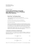
We seek a piecewise linear convex function φ as in (1) with φ(0) = 0. Such a
function has the form φ(x)=φ(a
k
)+α
k
(x − a
k
), x ∈ [a
k
,a
k+1
], with 0 = a
0
<
a
1
< <a
k
<a
k+1
→∞and increasing slopes α
k
↑∞.

Chapter I: Martingale Theory 7
The increasing property of the slopes α
k
implies that φ is convex. Observe that
φ(x) ≥ α
k
(x − a
k
), for all x ≥ a
k
.Thusα
k
↑∞implies φ(x)/x →∞,asx ↑∞.
We must choose a
k
and α
k
such that sup
i∈I
E(φ(|X
i
|)) < ∞.Ifi ∈ I, then
E(φ(|X
i
|)) =

∞
k=0
E


φ(|X
i
|); [a
k
≤|X
i
| <a
k+1
]

=

∞
k=0
E

φ(a
k
)+α
k
(|X
i
|−a
k
); [a
k
≤|X
i
| <a
k+1

]

≤

∞
k=0

φ(a
k
)P (|X
i
|≥a
k
)+α
k
E

|X
i
|;[|X
i
|≥a
k
]

.
Using the estimate P ([|X
i
|≥a
k

]) ≤ a
−1
k
E

|X
i
|;[|X
i
|≥a
k
]

and observing that
φ(a
k
)/a
k
≤ α
k
by the increasing nature of the slopes (Figure 1.1), we obtain
E(φ(|X
i
|)) ≤

∞
k=0
2α
k
E


|X
i
|;[|X
i
|≥a
k
]

≤

∞
k=0
2α
k
δ(a
k
).
Since δ(a) → 0, as a →∞, we can choose the sequence a
k
↑∞such that δ(a
k
) <
3
−k
, for all k ≥ 1. Note that a
0
cannot be chosen (a
0
= 0) and hence has to be

treated separately. Recall that δ(a
0
)=δ(0) < ∞ and choose 0 <α
0
< 2 so that
α
0
δ(a
0
) < 1=(2/3)
0
.Fork ≥ 1 set α
k
=2
k
. It follows that
E(φ(|X
i
|)) ≤

∞
k=0
2(2/3)
k
=6, for all i ∈ I.
1.b.6 Example. If p>1 then the function φ(x)=x
p
satisfies the assumptions
of Theorem 1.b.5 and E(φ(|X
i

|)) = E(|X
i
|
p
)=X
i

p
p
. It follows that a bounded
family F = {X
i
| i ∈ I }⊆L
p
(P ) is automatically uniformly integrable, that is,
L
p
-boundedness (where p>1) implies uniform integrability. A direct proof of this
fact is also easy:
1.b.7. Let p>1.IfK = sup
i∈I
X
i

p
< ∞, then the family {X
i
| i ∈ I }⊆L
p
is

uniformly integrable.
Proof. Let i ∈ I, c>0 and q be the exponent conjugate to p (1/p+1/q = 1). Using
the inequalities of Hoelder and Chebycheff we can write
E

|X
i
|1
[|X
i
|≥c]

≤1
[|X
i
|≥c]

q
X
i

p
= P

|X
i
|≥c

1
q

X
i

p
≤

c
−p
X
i

p
p

1
q
X
i

p
= c
−
p
q
K
1+
p
q
→ 0,
as c ↑∞, uniformly in i ∈ I.

8 2.a Sigma fields, information and conditional expectation.
2. CONDITIONING
2.a Sigma Þelds, information and conditional expectation. Let E(P ) denote the
family of all extended real valued random variables X on (Ω, F,P) such that
E(X
+
) < ∞ or E(X
−
) < ∞ (i.e., E(X) exists). Note that E(P )isnotavec-
tor space since sums of elements in E(X) are not defined in general.
2.a.0. (a) If X ∈E(P ), then 1
A
X ∈E(P ), for all sets A ∈F.
(b) If X ∈E(P ) and α ∈ R, then αX ∈E(P ).
(c) If X
1
,X
2
∈E(P ) and E(X
1
)+E(X
2
) is defined, then X
1
+ X
2
∈E(P ).
Proof. We show only (c). We may assume that E(X
1
) ≤ E(X

2
). If E(X
1
)+E(X
2
)
is defined, then E(X
1
) > −∞ or E(X
2
) < ∞. Let us assume that E(X
1
) > −∞
and so E(X
2
) > −∞, the other case being similar. Then X
1
,X
2
> −∞, P -as.
and hence X
1
+ X
2
is defined P -as. Moreover E(X
−
1
),E(X
−
2

) < ∞ and, since
(X
1
+ X
2
)
−
≤ X
−
1
+ X
−
2
, also E

(X
1
+ X
2
)
−

< ∞.ThusX
1
+ X
2
∈E(P ).
2.a.1. Let G⊆Fbe a sub-σ-field, D ∈Gand X
1
,X

2
∈E(P ) G-measurable.
(a) If E(X
1
1
A
) ≤ E(X
2
1
A
), ∀A ⊆ D, A ∈G, then X
1
≤ X
2
as. on D.
(b) If E(X
1
1
A
)=E(X
2
1
A
), ∀A ⊆ D, A ∈G, then X
1
= X
2
as. on D.
Proof. (a) Assume that E(X
1

1
A
) ≤ E(X
2
1
A
), for all G-measurable subsets A ⊆ D.
If P

[X
1
>X
2
] ∩ D

> 0 then there exist real numbers α<βsuch that the
event A =[X
1
>β>α>X
2
] ∩ D ∈Ghas positive probability. But then
E(X
1
1
A
) ≥ βP(A) >αP(A) ≥ E(X
2
1
A
), contrary to assumption. Thus we must

have P

[X
1
>X
2
] ∩ D

= 0. (b) follows from (a).
We should now develop some intuition before we take up the rigorous devel-
opment in the next section. The elements ω ∈ Ω are the possible states of nature
and one among them, say δ, is the true state of nature. The true state of nature
is unknown and controls the outcome of all random experiments. An event A ∈F
occurs or does not occur according as δ ∈ A or δ ∈ A, that is, according as the
random variable 1
A
assumes the value one or zero at δ.
To gain information about the true state of nature we determine by means
of experiments whether or not certain events occur. Assume that the event A
of probability P(A) > 0 has been observed to occur. Recalling from elementary
probability that P(B ∩ A)/P (A) is the conditional probability of an event B ∈F
given that A has occurred, we replace the probability measure P on F with the
probability Q
A
(B)=P (B ∩ A)/P (A), B ∈F, that is we pass to the probability
space (Ω, F,Q
A
). The usual extension procedure starting from indicator functions
shows that the probability Q
A

satisfies
E
Q
A
(X)=P (A)
−1
E(X1
A
), for all random variables X ∈E(P ).
At any given time the family of all events A, for which it is known whether they
occur or not, is a sub-σ-field of F. For example it is known that ∅ does not occur,