financial statement analysis tools

105
CHAPTER 4 Financial Statement
Analysis Tools
In previous chapters we have seen how the firm’s basic financial statements are constructed.
In this chapter we will see how financial analysts can use the information contained in the
income statement and balance sheet for various purposes.
Many tools are available for use when evaluating a company, but some of the most valuable
are financial ratios. Ratios are an analyst’s microscope; they allow us to get a better view of
the firm’s financial health than just looking at the raw financial statements. A ratio is simply a
comparison of two numbers by division. We could also compare numbers by subtraction, but
a ratio is superior in most cases because it is a measure of relative size. Relative measures
After studying this chapter, you should be able to:
1. Describe the purpose of financial ratios and who uses them.
2. Define the five major categories of ratios (liquidity, efficiency, leverage,
coverage, and profitability).
3. Calculate the common ratios for any firm by using income statement and
balance sheet data.
4. Use financial ratios to assess a firm’s past performance, identify its current
problems, and suggest strategies for dealing with these problems.
5. Calculate the economic profit earned by a firm.
CHAPTER 4: Financial Statement Analysis Tools
106
are more easily compared to previous time periods or other firms than changes in dollar
amounts.
Ratios are useful to both internal and external analysts of the firm. For internal purposes,
ratios can be useful in planning for the future, setting goals, and evaluating the performance
of managers. External analysts use ratios to decide whether or not to grant credit, to monitor
financial performance, to forecast financial performance, and to decide whether to invest in
the company.
We will look at many different ratios, but you should be aware that these are, of necessity,
only a sampling of the ratios that might be useful. Furthermore, different analysts may

calculate ratios slightly differently, so you will need to know exactly how the ratios are
calculated in a given situation. The keys to understanding ratio analysis are experience and
an analytical mind.
We will divide our discussion of the ratios into five categories based on the information
provided:
1. Liquidity ratios describe the ability of a firm to meets its short-term
obligations. They compare current assets to current liabilities.
2. Efficiency ratios describe how well the firm is using its investment in
various types of assets to produce sales. They may also be called asset
management ratios.
3. Leverage ratios reveal the degree to which debt has been used to finance
the firm’s asset purchases. These ratios are also known as debt
management ratios.
4. Coverage ratios are similar to liquidity ratios in that they describe the
ability of a firm to pay certain expenses.
5. Profitability ratios provide indications of how profitable a firm has been
over a period of time.
Before we begin the discussion of individual financial ratios, open your Elvis Products
International workbook from Chapter 2 and add a new worksheet named “Ratios.”
Liquidity Ratios
The term “liquidity” refers to the speed with which an asset can be converted into cash
without large discounts to its value. Some assets, such as accounts receivable, can easily be
converted into cash with only small discounts. Other assets, such as buildings, can be
converted into cash very quickly only if large price concessions are given. We therefore say
that accounts receivable are more liquid than buildings.
107
Liquidity Ratios
All other things being equal, a firm with more liquid assets will be more able to meet its
maturing obligations (e.g., its accounts payable and other short-term debts) than a firm with
fewer liquid assets. As you might imagine, creditors are particularly concerned with a firm’s

ability to pay its bills. To assess this ability, it is common to use the current ratio and/or the
quick ratio.
The Current Ratio
Generally, a firm’s current assets are converted to cash (e.g., collecting on accounts
receivable or selling its inventories) and this cash is used to retire its current liabilities.
Therefore, it is logical to assess a firm’s ability to pay its bills by comparing the size of its
current assets to the size of its current liabilities. The current ratio does exactly this. It is
defined as:
(4-1)
Obviously, the higher the current ratio, the higher the likelihood that a firm will be able to
pay its bills. So, from the creditor’s point of view, higher is better. However, from a
shareholder’s point of view this is not always the case. Current assets usually have a lower
expected return than do fixed assets, so the shareholders would like to see that only the
minimum amount of the company’s capital is invested in current assets. Of course, too little
investment in current assets could be disastrous for both creditors and owners of the firm.
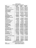
We can calculate the current ratio for 2011 for EPI by looking at the balance sheet (Exhibit
2-2, page 51). In this case, we have:
meaning that EPI has 2.39 times as many current assets as current liabilities. We will
determine later whether this is sufficient or not.
Exhibit 4-1 shows the beginnings of our “Ratios” worksheet. Enter the labels as shown. We
can calculate the current ratio for 2011 in B5 with the formula: h#BMBODF 4IFFUh#
h#BMBODF 4IFFUh#. After formatting to show two decimal places, you will see that
the current ratio is 2.39. Copy the formula to C5.
Current Ratio
Current Assets
Current Liabilities
=
Current Ratio
1,290.00
540.20

2.39 times==
CHAPTER 4: Financial Statement Analysis Tools
108
EXHIBIT 4-1
RATIO WORKSHEET FOR EPI
Notice that we have applied a custom number format (see page 51 to refresh your memory)
to the result in B5. In this case, the custom format is wYw. Any text that you include in
quotes will be shown along with the number. However, the presence of the text in the display
does not affect the fact that it is still a number and may be used for calculations. As an
experiment, in B6 enter the formula: #. The result will be 4.78 just as if we had not
applied the custom format. Now, in B7 type: Y and then copy the formula from B6 to
B8. You will get a #VALUE error because the value in B7 is a text string, not a number. This
is one of the great advantages to custom number formatting: We can have both text and
numbers in a cell and still use the number for calculations. Delete B6:B8 so that we can use
the cells in the next section.
The Quick Ratio
Inventories are often the least liquid of the firm’s current assets.
1
For this reason, many
believe that a better measure of liquidity can be obtained by excluding inventories. The
result is known as the quick ratio (sometimes called the acid-test ratio) and is calculated as:
(4-2)
For EPI in 2011 the quick ratio is:
Notice that the quick ratio will always be less than the current ratio. This is by design.
However, a quick ratio that is too low relative to the current ratio may indicate that
1. That is why you so often see 50% off sales when firms are going out of business.
Quick Ratio
Current Assets Inventories–
Current Liabilities
=

Quick Ratio
1,290.00 836.00–
540.20
0 . 8 4 t i m e s==
109
Efficiency Ratios
inventories are higher than they should be. As we will see later, this can only be determined
by comparing the ratio to previous periods or to other companies in the same industry.
We can calculate EPI’s 2011 quick ratio in B6 with the formula: h#BMBODF
4IFFUh#h#BMBODF 4IFFUh#h#BMBODF 4IFFUh#. Copying this
formula to C6 reveals that the 2010 quick ratio was 0.85. Be sure to remember to enter a
label in column A for all of the ratios.
Efficiency Ratios
Efficiency ratios, also called asset management ratios, provide information about how well
the company is using its assets to generate sales. For example, if two firms have the same
level of sales, but one has a lower investment in inventories, we would say that the firm with
lower inventories is more efficient with respect to its inventory management.
There are many different types of efficiency ratios that could be defined. However, we will
illustrate five of the most common.
Inventory Turnover Ratio
The inventory turnover ratio measures the number of dollars of sales that are generated per
dollar of inventory. It can also be interpreted as the number of times that a firm replaces its
inventories during a year. It is calculated as:
(4-3)
Note that it is also common to use sales in the numerator. Because the only difference
between sales and cost of goods sold is a markup (i.e., profit margin), this causes no
problems. In addition, you will frequently see the average level of inventories throughout the
year in the denominator. Whenever using ratios, you need to be aware of the method of
calculation to be sure that you are comparing “apples to apples.”
For 2011, EPI’s inventory turnover ratio was:

meaning that EPI replaced its inventories about 3.89 times during the year. Alternatively, we
could say that EPI generated $3.89 in sales for each dollar invested in inventories. Both
interpretations are valid, though the latter is probably more generally useful.
Inventory Turnover Ratio
Cost of Goods Sold
Inventory
=
Inventory Turnover Ratio
3,250.00
836.00
3.89 times==
CHAPTER 4: Financial Statement Analysis Tools
110
To calculate the inventory turnover ratio for EPI, enter the formula: h*ODPNF
4UBUFNFOUh#h#BMBODF 4IFFUh# into B8 and copy this formula to C8. Notice
that this ratio has deteriorated somewhat from 4 times in 2010 to 3.89 times in 2011.
Generally, high inventory turnover is considered to be good because it means that the
opportunity costs of holding inventory are low, but if it is too high the firm may be risking
inventory outages and the loss of customers.
Accounts Receivable Turnover Ratio
Businesses grant credit to customers for one main reason: to increase sales. It is important,
therefore, to know how well the firm is managing its accounts receivable. The accounts
receivable turnover ratio (and the average collection period) provides us with this information.
It is calculated by:
(4-4)
For EPI, the 2011 accounts receivable turnover ratio is (assuming that all sales are credit
sales):
So each dollar invested in accounts receivable generated $9.58 in sales. In cell B9 of your
worksheet, enter: h*ODPNF 4UBUFNFOUh#h#BMBODF4IFFUh#. The result is
9.58, which is the same as we found above. Copy this formula to C9 to get the 2010 accounts

receivable turnover ratio.
Whether or not 9.58 is a good accounts receivable turnover ratio is difficult to know at this
point. We can say that higher is generally better, but too high might indicate that the firm is
denying credit to creditworthy customers (thereby losing sales). If the ratio is too low, it
would suggest that the firm might be having difficulty collecting on its sales. We would have
to see if the growth rate in accounts receivable exceeds the growth rate in sales to determine
whether the firm is having difficulty in this area.
Average Collection Period
The average collection period (also known as days sales outstanding, or DSO) tells us how
many days, on average, it takes to collect on a credit sale. It is calculated as follows:
(4-5)
Accounts Receivable Turnover Ratio
Credit Sales
Accounts Receivable
=
Accounts Receivable Turnover Ratio
3,850.00
402.00
9.58 times==
Average Collection Period
Accounts Receivable
Credit Sales 360⁄
=
111
Efficiency Ratios
Note that the denominator is simply credit sales per day.
2
In 2011, it took EPI an average of
37.59 days to collect on their credit sales:
We can calculate the 2011 average collection period in B10 with the formula: h#BMBODF

4IFFUh#h*ODPNF 4UBUFNFOUh#. Copy this to C10 to find that in 2010
the average collection period was 36.84 days, which was slightly better than in 2011.
Note that this ratio actually provides us with the same information as the accounts receivable
turnover ratio. In fact, it can easily be demonstrated by simple algebraic manipulation:
Or alternatively:
Because the average collection period is (in a sense) the inverse of the accounts receivable
turnover ratio, it should be apparent that the inverse criteria apply to judging this ratio. In
other words, lower is usually better, but too low may indicate lost sales.
Many firms offer a discount for fast payment in order to get customers to pay more quickly.
For example, the credit terms on an invoice might specify 2/10n30, which means that there
is a 2% discount for paying within 10 days otherwise the entire balance is due in 30 days.
Such a discount is very attractive for customers, but whether it makes sense for a particular
firm is for them to decide. Remember that accounts receivable represents short-term loans
made to customers, and those funds have an opportunity cost. Regardless, offering a
discount will almost certainly reduce the average collection period and increase the accounts
receivable turnover.
Fixed Asset Turnover Ratio
The fixed asset turnover ratio describes the dollar amount of sales that are generated by each
dollar invested in fixed assets. It is given by:
2. The use of a 360-day year dates back to the days before computers. It was derived by assuming that
there are 12 months, each with 30 days (known as a “Banker’s Year”). You may also use 365 days;
the difference is irrelevant as long as you are consistent.
Average Collection Period
402.00
3,850.00 360⁄
37.59 days==
Accounts Receivable Turnover Ratio
360
Average Collection Period
=

Average Collection Period
360
Accounts Receivable Turnover Ratio
=
CHAPTER 4: Financial Statement Analysis Tools
112
(4-6)
For EPI, the 2011 fixed asset turnover is:
So, EPI generated $10.67 in revenue for each dollar invested in fixed assets. In your
“Ratios” worksheet, entering: h*ODPNF 4UBUFNFOUh#h#BMBODF 4IFFUh#
into B11 will confirm that the fixed asset turnover was 10.67 times in 2011. Again, copy this
formula to C11 to get the 2010 ratio.
Total Asset Turnover Ratio
Like the other ratios discussed in this section, the total asset turnover ratio describes how
efficiently the firm is using all of its assets to generate sales. In this case, we look at the
firm’s total asset investment:
(4-7)
In 2011, EPI generated $2.33 in sales for each dollar invested in total assets:
This ratio can be calculated in B12 on your worksheet with: h*ODPNF
4UBUFNFOUh#h#BMBODF 4IFFUh#. After copying this formula to C12, you
should see that the 2010 value was 2.34, essentially the same as 2011.
We can interpret the asset turnover ratios as follows: Higher turnover ratios indicate more
efficient usage of the assets and are therefore preferred to lower ratios. However, you should
be aware that some industries will naturally have lower turnover ratios than others. For
example, a consulting business will almost surely have a very small investment in fixed
assets and therefore a high fixed asset turnover ratio. On the other hand, an electric utility
will have a large investment in fixed assets and a low fixed asset turnover ratio. This does
not mean, necessarily, that the utility company is more poorly managed than the consulting
firm. Rather, each is simply responding to the demands of their very different industries.
Fixed Asset Turnover

Sales
Net Fixed Assets
=
Fixed Asset Turnover
3,850.00
360.80
10.67 times==
Total Asset Turnover
Sales
Total Assets
=
Total Asset Turnover
3,850.00
1,650.80
2.33 times==
113
Leverage Ratios
EXHIBIT 4-2
EPI’S FINANCIAL RATIOS
At this point, your worksheet should resemble the one in Exhibit 4-2. Notice that we have
applied the custom format, discussed above, to most of these ratios. In B10 and C10,
however, we used the custom format w EBZTw because the average collection period
is measured in days.
Leverage Ratios
In physics, leverage refers to a multiplication of force. Using a lever and fulcrum, you can
press down on one end of a lever with a given force and get a larger force at the other end.
The amount of leverage depends on the length of the lever and the position of the fulcrum. In
finance, leverage refers to a multiplication of changes in profitability measures. For
example, a 10% increase in sales might lead to a 20% increase in net income.
3

The amount
of leverage depends on the amount of debt that a firm uses to finance its operations, so a firm
that uses a lot of debt is said to be “highly leveraged.”
Leverage ratios describe the degree to which the firm uses debt in its capital structure. This
is important information for creditors and investors in the firm. Creditors might be
concerned that a firm has too much debt and will therefore have difficulty in repaying loans.
Investors might be concerned because a large amount of debt can lead to a large amount of
volatility in the firm’s earnings. However, most firms use some debt. This is because the tax
3. As we will see in Chapter 6, this would mean that the degree of combined leverage is 2.
CHAPTER 4: Financial Statement Analysis Tools
114
deductibility of interest can increase the wealth of the firm’s shareholders. We will examine
several ratios that help to determine the amount of debt that a firm is using. How much is too
much depends on the nature of the business.
The Total Debt Ratio
The total debt ratio measures the total amount of debt (long-term and short-term) that the
firm uses to finance its assets:
(4-8)
Calculating the total debt ratio for EPI, we find that debt financing makes up about 58.45%
of the firm’s capital structure:
The formula to calculate the total debt ratio in B14 is: h#BMBODF 4IFFUh#
h#BMBODF 4IFFUh#. The result for 2011 is 58.45%, which is higher than the 54.81%
in 2010.
The Long-Term Debt Ratio
Many analysts believe that it is more useful to focus on just the long-term debt (LTD) instead
of total debt. The long-term debt ratio is the same as the total debt ratio, except that the
numerator includes only long-term debt:
(4-9)
EPI’s long-term debt ratio is:
In B15, the formula to calculate the long-term debt ratio for 2011 is: h#BMBODF

4IFFUh#h#BMBODF 4IFFUh#. Copying this formula to C15 reveals that in
2010 the ratio was only 22.02%. Obviously, EPI has increased its long-term debt at a faster
rate than it has added assets.
Total Debt Ratio
Total Liabilities
Total Assets

Total Assets Total Equity–
Total Assets
==
Total Debt Ratio
964.81
1,650.80
58.45%==
Long-Term Debt Ratio
Long-Term Debt
Total Assets
=
Long-Term Debt Ratio
424.61
1,650.80
25.72%==
115
Leverage Ratios
The Long-Term Debt to Total Capitalization Ratio
Similar to the previous two ratios, the long-term debt to total capitalization ratio tells us the
percentage of long-term sources of capital that is provided by long-term debt (LTD). It is
calculated by:
(4-10)
For EPI, we have:

Because EPI has no preferred equity, its total capitalization consists of long-term debt and
common equity. Note that common equity is the total of common stock and retained
earnings. We can calculate this ratio in B16 of the worksheet with: h#BMBODF
4IFFUh#h#BMBODF 4IFFUh#h#BMBODF 4IFFUh#. In 2010 this
ratio was only 32.76%.
The Debt to Equity Ratio
The debt to equity ratio provides exactly the same information as the total debt ratio, but in a
slightly different form that some analysts prefer:
(4-11)
For EPI, the debt to equity ratio is:
In B17, this is calculated as: h#BMBODF 4IFFUh#h#BMBODF 4IFFUh#.
Copy this to C17 to find that the debt to equity ratio in 2010 was 1.21 times.
To see that the total debt ratio and the debt to equity ratio provide the same information,
realize that:
(4-12)
but from rearranging equation (4-8) we know that:
LTD to Total Capitalization
LTD
LTD Preferred Equity Common Equity++
=
LTD to Total Capitalization
424.61
424.61 685.99+
38.23%==
Debt to Equity
Total Debt
Total Equity
=
Debt to Equity
964.81

685.99
1 . 4 1 t i m e s==
Total Debt
Total Equity

Total Debt
Total Assets

Total Assets
Total Equity

×=
CHAPTER 4: Financial Statement Analysis Tools
116
(4-13)
so, by substitution we have:
(4-14)
We can convert the total debt ratio into the debt to equity ratio without any additional
information (the result is not exact due to rounding):
The Long-Term Debt to Equity Ratio
Once again, many analysts prefer to focus on the amount of long-term debt that a firm
carries. For this reason, many analysts like to use the long-term debt to total equity ratio:
(4-15)
EPI’s long-term debt to equity ratio is:
The formula to calculate EPI’s 2011 long-term debt to equity ratio in B18 is: h#BMBODF
4IFFUh#h#BMBODF 4IFFUh#. After copying this formula to C18, note that
the ratio was only 48.73% in 2010.
At this point, your worksheet should look like the one in Exhibit 4-3.
Coverage Ratios
The coverage ratios are similar to liquidity ratios in that they describe the quantity of funds

available to “cover” certain expenses. We will examine two very similar ratios that describe
the firm’s ability to meet its interest payment obligations. In both cases, higher ratios are
desirable to a degree. However, if they are too high, it may indicate that the firm is under-
utilizing its debt capacity and therefore not maximizing shareholder wealth.
Total Assets
Total Equity

1
1Total Debt Ratio–
=
Total Debt
Total Equity

Total Debt
Total Assets

1
1
Total Debt
Total Assets
–

×=
Total Debt
Total Equity
0.5845
1
1 0.5845–

× 1.41==

Long-Term Debt to Equity
LTD
Preferred Equity Common Equity+
=
Long-Term Debt to Equity
424.61
685.99
6 1 . 9 0 %==
117
Coverage Ratios
EXHIBIT 4-3
EPI’S FINANCIAL RATIOS WITH THE LEVERAGE RATIOS
The Times Interest Earned Ratio
The times interest earned ratio measures the ability of the firm to pay its interest obligations
by comparing earnings before interest and taxes (EBIT) to interest expense:
(4-16)
For EPI in 2011 the times interest earned ratio is:
In your worksheet, the times interest earned ratio can be calculated in B20 with the formula:
h*ODPNF 4UBUFNFOUh#h*ODPNF 4UBUFNFOUh#. Copy the formula to
C20 and notice that this ratio has declined rather precipitously from 3.35 in 2010.
Times Interest Earned
EBIT
Interest Expense
=
Times Interest Earned
149.70
76.00
1 . 9 7 t i m e s==
CHAPTER 4: Financial Statement Analysis Tools
118

The Cash Coverage Ratio
EBIT does not really reflect the cash that is available to pay the firm’s interest expense. That
is because a noncash expense (depreciation) has been subtracted in the calculation of EBIT.
To correct for this deficiency, some analysts like to use the cash coverage ratio instead of
times interest earned. The cash coverage ratio is calculated as:
(4-17)
The calculation for EPI in 2011 is:
Note that the cash coverage ratio will always be higher than the times interest earned ratio.
The difference depends on the amount of depreciation expense and therefore the amount and
age of fixed assets.
The cash coverage ratio can be calculated in cell B21 of your “Ratios” worksheet
with: h*ODPNF4UBUFNFOUh#h*ODPNF4UBUFNFOUh#h*ODPNF
4UBUFNFOUh#. In 2010, the ratio was 3.65.
Profitability Ratios
Investors, and therefore managers, are particularly interested in the profitability of the firms
that they own. As we’ll see, there are many ways to measure profits. Profitability ratios
provide an easy way to compare profits to earlier periods or to other firms. Furthermore, by
simultaneously examining the first three profitability ratios, an analyst can discover
categories of expenses that may be out of line.
Profitability ratios are the easiest of all the ratios to analyze. Without exception, high ratios
are preferred. However, the definition of high depends on the industry in which the firm
operates. Generally, firms in mature industries with lots of competition will have lower
profitability measures than firms in faster growing industries with less competition. For
example, grocery stores will have lower profit margins than computer software companies.
In the grocery business, a net profit margin of 3% would be considered quite good. That
same margin would be abysmal in the software business, where 15% or higher is common.
Cash Coverage Ratio
EBIT Noncash Expenses+
Interest Expense
=

Cash Coverage Ratio
149.70 20.00+
76.00
2.23 times==
119
Profitability Ratios
The Gross Profit Margin
The gross profit margin measures the gross profit relative to sales. It indicates the amount of
funds available to pay the firm’s expenses other than its cost of sales. The gross profit
margin is calculated by:
(4-18)
In 2011, EPI’s gross profit margin was:
which means that cost of goods sold consumed about 84.42% ( ) of sales
revenue. We can calculate this ratio in B23 with: h*ODPNF4UBUFNFOUh#
h*ODPNF4U BUFNFOUh#. After copying this formula to C23, you will see that the
gross profit margin has declined from 16.55% in 2010.
The Operating Profit Margin
Moving down the income statement, we can calculate the profits that remain after the firm
has paid all of its operating (nonfinancial) expenses.
The operating profit margin is calculated as:
(4-19)
For EPI in 2011:
The operating profit margin can be calculated in B24 with the formula: h*ODPNF
4UBUFNFOUh#h*ODPNF4UBUFNFOUh# . Note that this is significantly lower
than the 6.09% from 2010, indicating that EPI seems to be having problems controlling its
operating costs.
The Net Profit Margin
The net profit margin relates net income to sales. Because net income is profit after all
expenses, the net profit margin tells us the percentage of sales that remains for the
shareholders of the firm:

Gross Profit Margin
Gross Profit
Sales
=
Gross Profit Margin
600.00
3,850.00
15.58%==
10.1558–=
Operating Profit Margin
Net Operating Income
Sales
=
Operating Profit Margin
149.70
3,850.00
3.89%==
CHAPTER 4: Financial Statement Analysis Tools
120
(4-20)
The net profit margin for EPI in 2011 is:
which can be calculated on your worksheet in B25 with: h*ODPNF4UBUFNFOUh#
h*ODPNF4UBUFNFOUh#. This is lower than the 2.56% in 2010. If you take a look at
the common-size income statement (Exhibit 2-5, page 56), you can see that profitability has
declined because cost of goods sold, SG&A expense, and interest expense have risen more
quickly than sales.
Taken together, the three profit margin ratios that we have examined show a company that
may be losing control over its costs. Of course, high expenses mean lower returns for
investors, and we’ll see this confirmed by the next three profitability ratios.
Return on Total Assets

The total assets of a firm are the investment that the shareholders have made. Much like you
might be interested in the returns generated by your investments, analysts are often
interested in the return that a firm is able to get from its investments. The return on total
assets is:
(4-21)
In 2011, EPI earned about 2.68% on its assets:
For 2011, we can calculate the return on total assets in cell B26 with the formula:
h*ODPNF4UBU FNFOUh#h#BMBODF 4IFFUh#. Notice that this is more
than 50% lower than the 5.99% recorded in 2010. Obviously, EPI’s total assets increased in
2011 at a faster rate than its net income (which actually declined).
Net Profit Margin
Net Income
Sales
=
Net Profit Margin
44.22
3,850.00
1.15%==
Return on Total Assets
Net Income
Total Assets
=
Return on Total Assets
44.22
1650.80
2 . 6 8 %==
121
Profitability Ratios
Return on Equity
While total assets represent the total investment in the firm, the owners’ investment

(common stock and retained earnings) usually represent only a portion of this amount (some
is debt). For this reason, it is useful to calculate the rate of return on the shareholder’s
invested funds. We can calculate the return on (total) equity as:
(4-22)
Note that if a firm uses no debt, then its return on equity will be the same as its return on
assets. The more debt a firm uses, the higher its return on equity will be relative to its return
on assets (see Du Pont Analysis on page 122).
In 2011, EPI’s return on equity was:
which can be calculated in B27 with: h*ODPNF 4UBUFNFOUh#h#BMBODF
4IFFUh#. Again, copying this formula to C27 reveals that this ratio has declined from
13.25% in 2010.
Return on Common Equity
For firms that have issued preferred stock in addition to common stock, it is often helpful to
determine the rate of return on just the common stockholders’ investment:
(4-23)
Net income available to common is net income less preferred dividends. In the case of EPI,
this ratio is the same as the return on equity because it has no preferred shareholders:
For EPI, the worksheet formula for the return on common equity is exactly the same as for
the return on equity.
Return on Equity
Net Income
Total Equity
=
Return on Equity
44.22
685.99
6 . 4 5 %==
Return on Common Equity
Net Income Available to Common
Common Equity

=
Return on Common Equity
44.22 0–
685.99
6 . 4 5 %==
CHAPTER 4: Financial Statement Analysis Tools
122
Du Pont Analysis
The return on equity (ROE) is important to both managers and investors. The effectiveness
of managers is often measured by changes in ROE over time, and their compensation may be
tied to ROE-based goals. Therefore, it is important that they understand what they can do to
improve the firm’s ROE and that requires knowledge of what causes changes in ROE over
time. For example, we can see that EPI’s return on equity dropped precipitously from 2010
to 2011. As you might imagine, both investors and managers are probably trying to figure
out why this happened. The Du Pont system is one way to look at this problem.
The Du Pont system is a way to break down the ROE into its components so that
management can understand how to improve the firm’s ROE. Let’s first take another look at
the return on assets (ROA):
(4-24)
So, the ROA shows the combined effects of profitability (as measured by the net profit
margin) and the efficiency of asset usage (the total asset turnover). Therefore, ROA could be
improved by increasing profitability or by using assets more efficiently.
As mentioned earlier, the amount of leverage that a firm uses is the link between ROA and
ROE. Specifically:
(4-25)
Note that the second term in (4-25) is sometimes called the “equity multiplier” and from (4-
13) we know it is equal to:
(4-26)
Substituting (4-26) into (4-25) and rearranging we have:
(4-27)

We can now see that the ROE is a function of the firm’s ROA and the total debt ratio. If two
firms have the same ROA, the one using more debt will have a higher ROE.
We can make one more substitution to completely break down the ROE into its components.
Because the first term in (4-27) is the ROA, we can replace it with (4-24):
ROA
Net Income
Total Assets

Net Income
Sales

Sales
Total Assets

×==
ROE
Net Income
Equity

Net Income
Total Assets

Total Assets
Equity

×==
Total Assets
Total Equity

1

1Total Debt Ratio–

1
1
Total Debt
Total Assets
–
==
ROE
Net Income
Total Assets

1
Total Debt
Total Assets
–


÷=
123
Profitability Ratios
(4-28)
Or, to simplify it somewhat:
(4-29)
To prove this to yourself, in A30 enter the label: %V 1POU 30&. Now, in B30 enter the
formula: ###. The result will be 6.45% as we found earlier. Note that
if a firm uses no debt then the denominator of equation (4-29) will be 1, and the ROE will be
the same as the ROA.
Analysis of EPI’s Profitability Ratios
Obviously, EPI’s profitability has slipped rather dramatically in the past year. The sources of

these declines can be seen most clearly if we look at all of EPI’s ratios. At this point, your
worksheet should resemble the one in Exhibit 4-4.
The gross profit margin in 2011 is lower than in 2010, but not significantly (at least
compared to the declines in the other ratios). The operating profit margin, however, is
significantly lower in 2011 than in 2010. This indicates potential problems in controlling the
firm’s operating expenses, particularly SG&A expenses. The other profitability ratios are
lower than in 2010 partly because of the “trickle down” effect of the increase in operating
expenses. However, they are also lower because EPI has taken on a lot of extra debt in 2011,
resulting in interest expense increasing faster than sales. This can be confirmed by
examining EPI’s common-size income statement (Exhibit 2-5, page 56).
Finally, the Du Pont analysis of the firm’s ROE has shown us that it could be improved by
any of the following: (1) increasing the net profit margin; (2) increasing the total asset
turnover; or (3) increasing the amount of debt relative to equity. Our ratio analysis has
shown that operating expenses have grown considerably, leading to the decline in the net
profit margin. Reducing these expenses should be the primary objective of management.
Because the total asset turnover ratio is near the industry average, as we’ll soon see, it may
be difficult to increase this ratio. However, the firm’s inventory turnover ratio is
considerably below the industry average and inventory control may provide one method of
improving the total asset turnover. An increase in debt is not called for because the firm
already has somewhat more debt than the industry average.
ROE
Net Income
Sales

Sales
Total Assets

×
1
Total Debt

Total Assets
–
=
ROE
Net Profit Margin Total Asset Turnover×
1Total Debt Ratio–
=
CHAPTER 4: Financial Statement Analysis Tools
124
EXHIBIT 4-4
COMPLETED RATIO WORKSHEET FOR EPI
Financial Distress Prediction
The last thing that any investor wants to do is to invest in a firm that is nearing a bankruptcy
filing or about to suffer through a period of severe financial distress. Starting in the late
1960s and continuing today, scholars and credit analysts have spent considerable time and
effort trying to develop models that could identify such companies in advance. The best-
known of these models was created by Professor Edward Altman in 1968. We will discuss
Altman’s original model and a later one developed for privately held companies.
125
Financial Distress Prediction
The Original Z-Score Model
4
The Z-score model was developed using a statistical technique known as multiple
discriminant analysis. This technique creates a quantitative model that places a company
into one of two (or more) groups depending on the score. If the score is below the cutoff
point, it is placed into group 1 (soon to be bankrupt), otherwise it is placed into group 2. In
fact, Altman also identified a third group that fell into a so-called “gray zone.” These
companies could go either way, but should definitely be considered greater credit risks than
those in group 2. Generally, the lower the Z-score, the higher the risk of financial distress or
bankruptcy.

The original Z-score model for publicly traded companies is:
(4-30)
where the variables are the following financial ratios:
Altman reports that this model is 80–90% accurate if we use a cutoff point of 2.675. That is,
a firm with a Z-score below 2.675 can reasonably be expected to experience severe financial
distress, and possibly bankruptcy, within the next year. The predictive ability of the model is
even better if we use a cutoff point of 1.81. There are, therefore, three ranges of Z-scores:
We can easily apply this model to EPI in the Ratios worksheet. However, first note that we haven’t
supplied information regarding the market value of EPI’s common stock. In A31, enter the label:
.BSLFU 7BMVF PG &RVJUZ and in B31 enter . The market value of the equity is
found by multiplying the share price by the number of shares outstanding. Next, enter: ;4DPSF
4. See E. Altman, “Financial Ratios, Discriminant Analysis and the Prediction of Corporate
Bankruptcy,” Journal of Finance, September 1968. The models discussed in this section are from
an updated version of this paper written in July 2000: E. Altman, “Predicting Financial Distress of
Companies: Revisiting the Z-Score and ZETA Models.” This paper can be obtained from http://
www.defaultrisk.com/pp_score_14.htm.
X
1
= net working capital/total assets
X
2
= retained earnings/total assets
X
3
= EBIT/total assets
X
4
= market value of all equity/book value of total liabilities
X
5

= sales/total assets
Z < 1.81 Bankruptcy predicted within one year
1.81 < Z < 2.675 Financial distress, possible bankruptcy
Z > 2.675 No financial distress predicted
Z1.2X
1
1.4X
2
3.3X
3
0.6X
4
X
5
++++=
CHAPTER 4: Financial Statement Analysis Tools
126
into A32, and in B32 enter the formula:
h#BMBODF 4IFFUh#h#BMBODF 4IFFUh#h#BMBODF 4IFFUh
#h#BMBODF 4IFFUh#h#BMBODF 4IFFUh#h*ODPNF
4UBUFNFOUh#h#BMBODF 4IFFUh##h#BMBODF 4IFFUh
#h*ODPNF 4UBUFNFOUh#h#BMBODF 4IFFUh#.
If you’ve entered the equation correctly, you will find that EPI’s Z-score in 2011 is 3.92,
which is safely above 2.675, so bankruptcy isn’t predicted.
The Z-Score Model for Private Firms
Because variable X
4
in equation (4-30) requires knowledge of the firm’s market
capitalization (including both common and preferred equity), we cannot easily use the model
for privately held firms. Estimates of the market value of these firms can be made, but the

result is necessarily very uncertain. Alternatively, we could substitute the book value of
equity for its market value, but that wouldn’t be correct. Most publicly traded firms trade for
several times their book value, so such a substitution would seem to call for a new
coefficient for X
4
. In fact, all of the coefficients in the model changed when Altman
reestimated it for privately held firms.
The new model for privately held firms is:
(4-31)
where all of the variables are defined as before, except that X
4
uses the book value of equity
instead of market value. Altman reports that this model is only slightly less accurate than the
one for publicly traded firms when we use the new cutoff points shown below.
If we treat EPI as a privately held firm, its Z-score for 2011 is 3.35 and for 2010 is 3.55.
These scores show that EPI is not likely to file for bankruptcy anytime soon.
Using Financial Ratios
Calculating financial ratios is a pointless exercise unless you understand how to use them.
One overriding rule of ratio analysis is this: A single ratio provides very little information
and may be misleading. You should never draw conclusions from a single ratio. Instead,
several ratios, and other information, should support any conclusions that you make.
Bankruptcy predicted within one year
Financial distress, possible bankruptcy
No financial distress predicted
Z′ 0.717X
1
0.847X
2
3.107X
3

0.420X
4
0.998X
5
++++=
Z′ 1.21<
1.23 Z′ 2.90<<
Z′ 2.90>
127
Using Financial Ratios
With that precaution in mind, there are several ways that ratios can be used to draw
important conclusions.
Trend Analysis
Trend analysis involves the examination of ratios over time. Trends, or the lack of trends,
can help managers gauge their progress toward a goal. Furthermore, trends can highlight
areas in need of attention. While we don’t really have enough information on Elvis Products
International to perform a trend analysis, it is obvious that many of its ratios are moving in
the wrong direction.
For example, all of EPI’s profitability ratios have declined in 2011 relative to 2010, some
rather dramatically. Management should immediately try to isolate the problem areas. For
example, the gross profit margin has declined only slightly, indicating that increasing
materials costs are not a major problem, though a price increase may be called for. The
operating profit margin has fallen by about 36%, and since we can’t blame increasing costs
of goods sold, we must conclude that operating costs have increased at a more rapid rate than
revenues. The common-size income statement (Exhibit 2-5, page 56) shows that the culprit
is SG&A expense. This increase in operating costs has led, to a large degree, to the decline
in the other profitability ratios.
One potential problem area for trend analysis is seasonality. We must be careful to compare
similar time periods. For example, many firms generate most of their sales during the
holidays in the fourth quarter of the year. For this reason they may begin building inventories

in the third quarter when sales are low. In this situation, comparing the third-quarter
inventory turnover ratio to the fourth-quarter inventory turnover would be misleading.
Comparing to Industry Averages
Aside from trend analysis, one of the most beneficial uses of financial ratios is to compare
similar firms within a single industry. This can be done by comparing to industry average
ratios, which are published by organizations such as the Risk Management Association
(RMA) and Standard & Poor’s. Industry averages provide a standard of comparison so that
we can determine how well a firm is performing relative to its peers.
Consider Exhibit 4-5, which shows EPI’s ratios and the industry averages for 2011. You can
enter the industry averages into your worksheet starting in D3 with the label: *OEVTUSZ
. Now select D5:D28, type  into D5, and then press the Enter key. Notice that the
active cell will change to D6 as soon as the Enter key is pressed. This is an efficient method
of entering a lot of numbers because your fingers never have to leave the number keypad.
This technique is especially helpful when entering numbers into multiple columns and
discontiguous cells.
CHAPTER 4: Financial Statement Analysis Tools
128
EXHIBIT 4-5
EPI’S RATIOS VS. INDUSTRY AVERAGES
It should be obvious that EPI is not being managed as well as the average firm in the
industry. From the liquidity ratios we can see that EPI is less able to meet its short-term
obligations than the average firm, though they are probably not in imminent danger of
missing payments. The efficiency ratios show us that EPI is not managing its assets as well
as would be expected, especially inventories. It is also obvious that EPI is using substantially
more debt than its peers. The coverage ratios indicate that EPI has less cash to pay its interest
expense than the industry average. This is due to carrying more than average debt. Finally,
all of these problems have led to subpar profitability measures, which seem to be getting
worse, rather than better.
It is important to note that industry averages may not be appropriate in all cases. In many
cases, it is probably more accurate to define the “industry” as the target company’s most

129
Using Financial Ratios
closely related competitors. This group is probably far smaller (maybe only three to five
companies) than the entire industry as defined by the 4-digit SIC code. The newer 6-digit
NAICS codes
5
improves, but doesn’t eliminate, this situation.
Company Goals and Debt Covenants
Financial ratios are often the basis of company goal setting. For example, a CEO might
decide that one goal of the firm should be to earn at least 15% on equity (ROE = 15%).
Obviously, whether or not this goal is achieved can be determined by calculating the return
on equity. Further, by using trend analysis, managers can gauge progress toward meeting
goals, and they can determine whether the goals are realistic or not.
Another use of financial ratios can be found in covenants loan to contracts. When companies
borrow money, the lenders (bondholders, banks, or other lenders) place restrictions on the
company, very often tied to the values of certain ratios. For example, the lender may require
that the borrowing firm maintain a current ratio of at least 2.0. Or, it may require that the
firm’s total debt ratio not exceed 40%. Whatever the restrictions, it is important that the firm
monitor its ratios for compliance, or the loan may be due immediately.
Automating Ratio Analysis
Ratio analysis is as much art as science, and different analysts are likely to render somewhat
different judgements on a firm. Nonetheless, you can have Excel do a rudimentary analysis
for you. Actually, the analysis could be made quite sophisticated if you are willing to put in
the effort. The technique that we will illustrate is analogous to creating an expert system,
though we wouldn’t call it a true expert system at this point.
An expert system is a computer program that can diagnose problems or provide an analysis
by using the same techniques as an expert in the field. For example, a medical doctor might
use an expert system to diagnose a patient’s illness. The doctor would tell the system about
the symptoms and the expert system would consult its rules to generate a likely diagnosis.
Building a true ratio analysis expert system in Excel would be very time consuming, and

there are better tools available. However, we can build a very simple system using only a
few functions. Our system will analyze each ratio separately and will only determine
whether a ratio is “Good,” “Ok,” or “Bad.” To be really useful, the system would need to
consider the interrelationships between the ratios, the industry that the company is in, and so
on. We leave it to you to improve the system.
5. North American Industry Classification System. This system was created by the U.S. Census
Bureau and its Canadian and Mexican counterparts in 1997 and is replacing the SIC codes. See
for more information.