THE IMPACT OF PARENTAL INCOME AND EDUCATION ON CHILD HEALTH: FURTHER EVIDENCE FOR ENGLAND doc
Bạn đang xem bản rút gọn của tài liệu. Xem và tải ngay bản đầy đủ của tài liệu tại đây (357.2 KB, 33 trang )
!
"
#
!
% &
*+
'+ '
&
,
&
,
'
! ! "#
% &
'
$
'%( '
)
/
"#
'
$
- .
0
&
-
& "
1 .
1 .
*
1 1 .
"
0
2 3 5
! 4
6)
6
.
7
This paper is produced as part of the Human Development and Public Policy research programme at Geary; however the views expressed here do not necessarily reflect those of
the Geary Institute. All errors and omissions remain those of the author.
Corresponding author: E-mail: Tel: 00353 1 7164637, Fax 00353 1 7161108
Geary WP/6/2007
1
Abstract
This paper investigates the robustness of recent findings on the effect of parental
education and income on child health. We are particularly concerned about spurious
correlation arising from the potential endogeneity of parental income and education.
Using an instrumental variables approach, our results suggest that the parental income
and education effects are generally larger than are suggested by the correlations
observed in the data. Moreover, we find strong support for the causal effect of income
being large for the poor, but small at the average level of income.
JEL Classifications: I1
Keywords:
Child health; Intergenerational Transmission
Geary WP/6/2007
2
1.
Introduction
There is a vast literature documenting the relationship between socioeconomic
status (SES) and health (see, for example, Wilkinson and Marmot 2003). Specifically
the relationship between the health of children and the income of their parents has
been the focus of much research. This relationship is important because it has been
shown that the effects are long-lasting - poor health in childhood is associated with
lower educational attainment, inferior labour market outcomes and worse health later
in life.1 Case, Lubotsky and Paxson (2002) and Currie, Shields and Wheatley-Price
(2004) investigate the role of parental income, in the US and UK respectively, and
find that there is an effect on child health. They refer to this income effect as the
“gradient”. The US data suggest that this gradient is larger for older children while the
UK data suggests that is not the case - this discrepancy is perhaps due to the freely
available healthcare in the UK.
The key contribution of this paper is to investigate the robustness of the main
UK results presented in Currie et al., (2004) to the possible endogeneity of parental
income and education. In particular, this paper adopts an instrumental variables (IV)
solution to spurious correlation and measurement error. In addition to considering the
impact of parental education and income on parent or self-reported child health, we
also investigate their impact on chronic health conditions. This study also explores the
possibility that the effect of income is different (presumably larger) for poorer
households – an argument that is frequently suggested in the literature, but seldom
explicitly tested.
Our analysis is based on a sample of 6,389 children drawn from the Health
Survey for England. We find that, in support of earlier work, there is a significant
income gradient on self-reported health, but there is no significant interaction with
child age once one purges income (and education) of its endogenous variation.
Moreover, the effects are stronger once we allow for income and education to be
endogenous. Finally, we find support for the idea that the causal effects of income are
strongest for the poorest. Any effects on having a chronic health condition seem
confined to young children.
1
Marmot and Wadsworth (1997) identify several “pathways” whereby childhood health affects adult
health. See also Currie and Hyson (1999), Case et al., (2002), Currie (2004) and Graham and Power
(2004).
Geary WP/6/2007
3
First and foremost, we are concerned that the income effects on child health,
which have been found in earlier studies, may be the result of a spurious correlation
rather than a causal mechanism. This can arise due to endogeneity (i.e. reverse
causation arising from a sick child reducing parental income, or from low income
parents and sick children having some common unobservable cause) or from
measurement error (not least because the income data are grouped). In the case of
reverse causation, we would expect least squares estimates of the income effect to be
biased upwards since income would capture the effect of income and the effect of
other factors that are correlated with income, but which are not included in the model.
However, measurement error (in income) may cause the correlation to understate the
true effect and, in general, we cannot sign the direction of bias. It should be noted that
IV methods will, unlike OLS, yield estimates of local, rather than average, effects.2,3
Secondly, we are conscious that a similar argument can be made for the effect
of education - if education and child health are correlated with some common
unobservable (say, low time preference) then least squares estimates of the effect of
parental education will be biased.4 Omitting income from such analyses will cause the
education coefficient to be biased upwards, to the extent that income and health are
positively correlated. In some cases, it is useful to know the effect of education on
health, without holding income constant – for example, we may wish to know the
extent to which the effect of an education reform affects health, both directly and
indirectly via the effect of education increasing income. However, in other cases, it is
useful to disaggregate the overall effect so as to isolate the effect of income alone,
holding education constant: for example, if one is interested in the likely effect of
changes in income transfers to parents on child health. The interpretation of the
income effect may be different when education is controlled for – education may pick
up the permanent component of income so that the coefficient of current income can
then be interpreted as current income shocks.
2
See Imbens and Angrist (1994).
3
Panel data has been used to control for unobservable fixed effects in a few studies (see Adams, Hurd,
McFadden, Merrill and Ribeiro (2003), Frijters, Haisken-DeNew and Shields (2003), Meer, Miller and
Rosen (2003) and Contoyannis, Jones and Rice (2004)) but only in the context of adult health. These
suggest little support for a causal effect of income. We know of no studies that exploit sibling
differences.
4
A number of studies have addressed the issue of education endogeneity using instrumental variable
techniques but only in the context of adult health (see, for example, Berger and Leigh 1989; LlerasMuney 2005 and Arkes 2003).
Geary WP/6/2007
4
In addition, there is a well developed literature, albeit mostly in a development
context, that maternal background is more important than paternal.5 We therefore
examine the impact of both paternal and maternal education on child health outcomes,
with and without income included in the specification.
Parental income data are often grouped and, in cases where the range midpoint
is used, income is measured with error and the coefficient on income will be biased
towards zero. It is difficult to construct a likely argument as to why measurement
error in parental incomes should vary by the age of the child, so for example, the
result in Case et al., (2002) of a significantly positive interaction effect between child
age and parental income is likely to be robust to any measurement error in income.
However, the strength of any reverse causation may well vary with child age. For
example, a sick child may require greater parental care when young, which may imply
a larger reduction in parental labour supply and income consequently. In which case,
the extent of downward bias in the income effect obtained from least squares
estimation ought to be larger for households with young children relative to older
children. This might account for the changing gradient by age. However, it may well
be possible to construct arguments that go in the opposite direction and the question
ultimately becomes an empirical one that can only be resolved through obtaining
unbiased coefficients using some alternative method to least squares.
Finally, the paper explores the possibility that income effects may be
nonlinear, such that the income effect diminishes with income.
This paper is structured as follows: Section 2 outlines the existing literature.
Section 3 describes the data. Section 4 presents and discusses the results, and Section
5 concludes.
2.
Literature
There are a variety of potential disadvantages for children from having low
parental income and at least some of these may have long-lasting, and even
5
A number of studies have noted that maternal factors can affect a wide range of child outcomes
including educational choices (Simpson 2003; Chevalier, Harmon, O’Sullivan, Walker 2005), cognitive
and social development (Menaghan and Parcel 1991), political orientations (McAdams, VanDyke,
Munch, Shockey 1997) and religiosity (Kieren and Munro 1987).
Geary WP/6/2007
5
permanent, effects.6 However, the mechanisms by which income is related to health
remain controversial and, as noted by Deaton and Paxson (1998), “there is a welldocumented but poorly understood gradient linking socio-economic status to a wide
range of health outcomes” (p. 248). Case et al., (2002) analyse the relationship
between family income and child health using the US National Health Interview
Survey (NHIS).7 They show the existence of a significant and positive effect of
income, with children in poorer families having significantly worse health than
children from richer families. In addition, they find that the income gradient in child
health increases with child age in the US, with the protective effect of income
accumulating over the childhood years.8 They suggest that this effect operates partly
through poorer children with chronic health conditions such as asthma and diabetes
having worse health. In an attempt to address why poorer children should be more
afflicted by these conditions, they find that a genetic explanation, whereby parents
who are in poor health earn less and have less healthy children, does not successfully
explain the results. They also find that health insurance does not play a role.
Case, Fertig and Paxson (2005) investigate the relationship between parental
SES and child health for the UK using the National Child Development Study
(NCDS) 1958 birth cohort. They find that the relationship between parental SES and
child health gets steeper as children get older – i.e. the health differences across SES
gets larger as children age. However it remains unclear what causal mechanism lies
behind this result. For example, it is not clear whether this is due to low SES children
having more adverse health shocks, or more serious ones, or whether such households
do not cope as well with these shocks. Currie and Hyson (1999) partially succeed in
addressing a similar issue using US data - for low birthweight. They find that
birthweights are lower for babies from low SES households but, surprisingly, the
effect of low birthweight on health did not vary much across SES. They suggest that
6
See Case and Paxson (2006) for a review of the evidence relating child health to subsequent lifetime
outcomes.
7
In addition to the children in the 1986-1995 National Health Interview Survey (NHIS) cross-section
dataset, this study also used the Panel Study of Income Dynamics (PSID), and the National Health and
Nutrition Examination Survey from 1988 and 1994. The NHIS has large sample sizes and so permits
the analysis of conditions that are relatively rare, while the PSID allows the effect of household income
over time to be investigated.
8
Currie and Stabile (2003) replicate this result for Canada, and also found evidence of an increasing
income effect that increased with child age, which they attributed to low income children experiencing
more health shocks than high income children.
Geary WP/6/2007
6
health is a potentially important transmission mechanism for the intergenerational
correlation of income and education.
Case et al., (2002) find that not only do children from poorer households
suffer from worse health, but also that these adverse health effects tend to compound
over time so that the variation in health across income or social class increases with
age, even across children with similar chronic conditions. This results in children of
poorer households entering adulthood in worse health and with more serious chronic
conditions. It appears their results do not arise because higher income parents tend to
have more education. They find that this income gradient remains even after
controlling for parental education, and that education has an independent positive
effect on health. Despite the common finding that income effects on child outcomes
are larger at lower levels of income, they find that the gradient appears at all income
levels; upper-income children do better than middle-income children, and middleincome children do better than lower-income children. The authors also find that the
disparities in child health by parental income become larger with child age. Even after
controlling for parental education, doubling household income increases the
probability that a child aged 0–3 (4-8, 9-12, 13-17) is in excellent or very good health
by about 4 percent (5 percent, 6 percent, 7 percent). They go on to investigate chronic
conditions, such as asthma, other respiratory conditions, kidney disease, heart
conditions, diabetes, digestive disorders, and mental health conditions. Poor children
with chronic conditions have poorer health than do higher-income children with the
same conditions. Finally, they examine whether it is only permanent income that
matters or, rather, whether the timing of income matters such that, for example, low
income in early childhood has a more adverse effect on later health than low income
later in childhood and they find no effect of the timing of income.
Recent work by Currie, Shields and Wheatley-Price (2004) also investigates
the relationship between the health of children and the incomes (and education levels)
of their parents, using pooled data from the 1997-2002 Health Surveys of England
(HSE, see Sprosten and Primatesta, 2003). In this data two generations are present in
the household, therefore it is possible to match the health of children with the
educational attainment and income of their parents. This study attempted to confirm
the extent to which findings for the US, in the earlier research by Case et al., (2002),
also hold in England.
Geary WP/6/2007
7
Like Case et al., (2002), Currie et al., (2004) find robust evidence of an
income gradient using subjectively assessed general health status, both controlling for
parental education and not. However, the size of this gradient is somewhat smaller
than in Case et al., (2002). Moreover, they find no evidence that the income gradient
increases with child age. They find statistically significant income effects on the
probability of having some chronic health conditions - notably asthma, mental and
other nervous system problems, and skin complaints, which have a higher incidence
in poorer families. There is some evidence that income does ‘protect’ children from
the adverse general health consequences of some conditions such as mental illness
and other nervous system problems, metabolic problems such as diabetes, and blood
pressure problems such as hypertension. Independent effects of parental education,
especially the mother’s, on the health of children were also found.9 However, they
failed to find a significant interaction between child age and parental income –
something which they attribute to the success of the National Health Service (NHS) in
the UK. While both Case et al., (2002) and Currie et al., (2004) show that their
income gradient results are robust to including other observable parental
characteristics and lifestyle variables, there remains the possibility that unobservable
factors might still account for the results.
Burgess, Propper and Rigg et al., (2004) use an early 1990’s cohort of children
from a particular part of South West England and find the direct impact of income on
child health is small. They also find no change in the income gradient with child
age.10
Unlike the US, where private health insurance is the norm, the UK has had a
National Health Service with health care being free at the point of delivery since 1948
(see Culyer and Wagstaff 1993).
Currie et al., (2004) argue that the NHS is
successful in insuring the health of the children of low income UK parents as they,
unlike Case et al (2002), find no evidence that the income effect on child health
increases with child age.11 They also extend the findings of US research in a number
9
Additionally, they found that a significant income gradient remains after controlling for family fixed
effects, child diet and parental exercise.
10
Emerson et al., (2005) use a UK survey of child mental health to demonstrate a correlation with
household income.
11
Currie et al., (2004) do not, however, argue that there is no income effect at all - although the logic
of their argument should apply for pre-natal child health as well, since NHS is a “cradle to grave”
service that ought to ensure maternal health before and during pregnancy.
Geary WP/6/2007
8
of important ways. For example, they find clear effects of vegetable consumption and
physical exercise on child health, but controlling for these, they find that their income
effect results are largely unchanged. They also show that an income effect exists for
objective measures of child health, derived from anthropometrical measurements and
blood samples.
Very few studies examine the effect of exogenous income variation on child
outcomes. Some studies exploit experimental welfare reforms - for example, Morris
and Gennetian (2003) and Chase-Lansdale et al., (2003) look at the effects of
experimental and non-experimental welfare reforms in the US on child outcomes and
generally find favourable effects. The only study, to our knowledge, that considers the
effects of natural experimental variation in lump-sum income is due to Costello et al.,
(2003) who track the mental health and behaviour of Native American Indian children
before and after the opening of a casino that resulted in large lump-sum transfers
being made to these parents.12 The control group was the children of other (nonNative American) poor parents in the same counties. Both treatment and control
groups benefited from the improvement in the job market associated with the casino
opening.
Brooks-Gunn and Duncan (1997) lament the paucity of evidence on
exogenous income variation and refer to the income maintenance experiments that
occurred in several places in the US during the 1960’s and 70’s. They note that only
in the poorest area (rural North Carolina) were there significant effects on child
health, suggesting that the effect of income may be confined to just the children of
low income parents. Although there seems to be a presumption in the literature that
the effects of income are largest for the poorest, very few studies investigate the
possibility of such nonlinearity explicitly and this is something we explore in our
analysis below.13
12
Many parents also increased their labour supply but the effects for those that did not were similar to
those that did suggesting that it was income that mattered.
13
The review in Blau (1999) suggests that there is little evidence of any diminution in the effect of
income as income rises.
Geary WP/6/2007
9
3.
Data and sample selection
The Health Survey for England (HSE) was initiated by the British
government’s Department of Health in 1992 to monitor trends in the nation’s health.14
The HSE surveys are an important source of information on household and individual
characteristics and both subjective and objective measures of health. Each survey uses
the Postcode Address File as a sampling frame, and is collected by a combination of
face-to-face interviews, self-completed questionnaires and medical examinations.
Each year the survey over-samples particular groups – for example, the elderly, ethnic
minorities, etc. and our analysis applies sampling weights to produce the correct
standard errors.
Although the HSE was initiated in 1992, the sample used in this paper only
includes surveys from 1997-2002, since information on children aged 2-15 was only
collected from 1995 onwards15 (the 2001 survey extended the analysis to children
under the age of 2) and household income was only collected from 1997 onwards. As
children and parents from the same household are interviewed we are able to match
parental characteristics to the child’s record.16 Pooling the six surveys resulted in a
dataset containing 26,498 children; however as the parents of the over-sampled
children included in 1997 and 2002 surveys were not interviewed our sample size is
substantially reduced to 16,175. In addition, unlike Currie et al., (2004) we exclude
children whose fathers or mothers are either missing from the survey or are missing
from the household (i.e. one-parent families), and we also drop those whose parents
self-report themselves as being in an ethnic minority.17 These criteria reduce our
sample size to 9,958 children. We then drop any observations where data are missing
on our variables of interest: for example household income is missing for
approximately 10 percent of the sample. Our final sample therefore includes 6,389
children aged between 0 and 15, 19% of which are aged 0-3, 35% aged between 4-8,
14
The HSE are carried out by the Joint Health Surveys Unit of the National Centre for Social Research
and the Department of Epidemiology and Public Health, Royal Free and University College London.
Scotland, Northern Ireland and Wales have separate administrative arrangements for health care and
the HSE only covers England. There is a separate Scottish Health Survey.
15
Up to two randomly selected children per household are surveyed.
16
The HSE data does distinguish between natural, adoptive, foster and step parents and we define a
“parent” as any type of parent.
17
It seems likely that single mothers and ethnic minorities will exhibit different relationships to the
explanatory variables than white couples. Unfortunately the dataset is too small to sustain separate
analyses of these groups.
Geary WP/6/2007
10
27% between 9-12, and 19% between13-15.18 Table 1 describes the summary
statistics for the sub-sample used in the analysis. The average age that fathers left
school (17.36) is slightly higher than mothers (17.33) and, as expected, the average
age of fathers is approximately 2 years greater than that of mothers.
The primary variable of interest in this paper is a subjective measure of
children’s general health. It is a self-reported measure for children aged between 13
and 15 and is reported by parents for children less than 13 years of age. The variable
is based on responses to the question “How is your health in general?. Possible
answers range from Very Good to Very Bad on a 1 to 5 scale. Following Currie et al.,
(2004) the measure was recoded into a 4-category variable, whereby “Bad” and
“Very Bad” were combined due to low sample sizes in these categories. The
distribution of our dependent variable is as follows: Very Good (60.8 %), Good (33.9
%), Fair (4.7 %), Very Bad/Bad (0.5 %). The surveys also include information on
whether the child has a long-term chronic health condition (CHC). The respondent
can list up to 6 CHCs from the 42 categories that are coded. In our sample of 6,389
children, 20.9 percent have at least one chronic health condition. Thus, we also
include an analysis of chronic condition incidence. Figures 1 and 2 show the joint
distributions of self-reported health and child age, and the incidence of having a CHC
and child age. Note that both subjective ill health and having a chronic condition
increase as children age.
Following Currie et al., (2004) current total pre-tax annual family income is
used as a measure of parental income. It is coded in 31 income bands ranging from
less than £520 to more than £150,000. The midpoints of each band were taken and
deflated to 2000 prices using the UK average earnings19 index according to the month
in which the interview was conducted20. The average annual household real income is
£34,869.21,22
18
Full details of the original HSE data, and the (small) impact of our selection criteria, are available in
Table A1 in the appendix..
19
We follow Currie et al in deflating by an earnings index, and we also follow them in using incomes
of £520 and £150,000 for the bottom and top codes of the income distribution.
20
Estimates using the grouped dependent variable estimator due to Stewart (1983) were also conducted
and the results were unchanged.
Geary WP/6/2007
11
Our measure of parental schooling is derived from two sources. The HSE asks
parents the age at which they finished full-time education. It is coded 1-8 (where
1=Not yet finished, 2=Never went to school, 3= aged 14 or under, 4=aged 15, 5=
aged 16, 6= aged 17, 7=aged 18 and 9=aged 19 or over). As there are no parents in
the dataset who were old enough to have left school at age 14 (the minimum schoolleaving age prior to the 1958 increase), and as we drop ethnic minorities from our
sample, there is no one in our sample who left education before age 15. Furthermore,
as the variable is top coded at 19, we use an additional HSE variable which captures
the parents highest educational qualification to distinguish parents who left at 19 from
those who left after 19. We combine this with information from the UK Labour Force
Survey to determine the average leaving age of individuals with a degree.23 This
allows us to create a new age left school variable ranging from 15 to 21.24
21
Note that this figure is greater than Currie et al., (2004) findings as we only include households with
two parents, while Currie et al. also include single-parent households. We use the log of household
income in the empirical analysis.
22
Indeed the Labour Force Survey provides an important point of comparison to gauge the reliability of
the HSE data in regards the parental income and educational measures. Therefore, we compare our
HSE sample to a similar, but much larger, selected sample in the UK Labour Force Survey from 19972002. We attempt to replicate the HSE sample by analysing white two-parent households in England
who have children between the ages 0 and 15. Unlike the HSE, the household income measure in LFS
is continuous and represents a combination of mothers and fathers income. The average real household
income of £34,889 in LFS is almost the same as the HSE measure (£34,869). Appendix Figures A1a
and A1b show that the distribution of income (as reported in the 31 income bands in the HSE and
equivalent income bands imposed on LFS) is similar across both samples.
23
The HSE data contain two education measures – the age at which the respondent left school (which
is top coded at 19) and the respondent’s highest qualification level. The LFS data also contain the same
two measures, however the age left school variable is not top coded. To overcome the top-coding
problem within HSE, we use the LFS data to generate the average age of a respondent with a degree
(age 21), and the average age of a respondent with a teaching qualification (age 20). Then, for
respondents within HSE who have a degree or a teaching qualification, we recode their age left
education variable with the average age left education generated from the LFS data. Therefore the new
age left education variable the HSE data ranges from 14 to 21.
24
As already noted, one particular concern with the HSE data is that the educational measure, which
reports the age at which the parent left full-time education, has an upper bound at age 19; therefore we
cannot distinguish different levels of higher education. The LFS data, on the other hand, include a
continuous educational measure. Table A1 in the Appendix compares the age at which mothers and
fathers left full-time education in both the LFS and HSE samples. It shows that the majority of mothers
(43.21 percent in LFS and 43.51 percent in HSE) and fathers (46.98 percent in LFS and 43.71 percent
in HSE) left education at 16. There are notable similarities between the two datasets. While a direct
comparison of the upper age categories is not possible, Table A1 shows that 25.47 percent of fathers
and 23.41 percent of mothers in the LFS left education at 19 or over, compared with 28.23 percent and
23.27 percent in the HSE. Appendix Figures A2a-A2d report the corresponding histograms.
Geary WP/6/2007
12
Figure 1
Self-reported child (ill) health and age of child
Subjective Child Health
0
.2
Proportion
.4
.6
by age category
0-3
4-8
9-12
Very Good
Fair
Figure 2
13-15
Good
Poor
Having a chronic health condition and age of child
Child Chronic Health Condition (CHC)
0
Mean Chronic Health Condition
.05
.1
.15
.2
.25
by age category
0-3
Geary WP/6/2007
4-8
13
9-12
13-15
Table 1
Descriptive Statistics HSE 1997-2002 - Estimation Sample
Child’s subjective ill health (1-5)
Child has a chronic health condition
All Ages
1.45
0-3
1.45
4-8
1.42
9-12
1.42
0.22
(0.61)
(0.62)
(0.61)
0.21
0.16
0.20
(0.58)
13-15
1.55
(0.64)
0.25
(0.41)
(0.37)
(0.40)
(0.42)
(0.43)
Household log income
10.25
10.22
10.25
10.26
10.29
Mother’s schooling
17.33
3.74
3.38
3.24
Father’s schooling
17.36
Mother’s age at birth
29.02
(5.14)
(5.25)
(5.10)
(0.66)
(1.82)
(1.88)
3.74
(0.65)
(1.77)
3.39
(0.69)
(1.81)
3.27
(0.63)
2.98
(1.80)
3.06
(2.04)
(1.77)
(2.03)
(2.09)
30.0
29.29
28.43
28.42
Father’s age at birth
31.21
32.17
31.64
30.56
30.44
Mother started smoking before age 16
0.15
0.15
0.14
0.15
Mother started smoking between ages
16 and 19
Mother started smoking after age 19
Father started smoking before age 16
Father started smoking between ages
16 and 19
Father started smoking after age 19
Mother smokes
Father smokes
Years exposed to Mother’s smoking
Years exposed to Father’s smoking
Mother smoked when pregnant
Paternal grandfather smoked
Paternal grandmother smoked
Maternal grandfather smoked
Maternal grandmother smoked
Mother affected by RoSLA
Father affected by RoSLA
(2.04)
(0.68)
(6.00)
(0.36)
0.20
(0.40)
0.08
(0.28)
0.26
(0.44)
0.21
(0.40)
0.09
(0.29)
0.24
(0.42)
0.24
(0.43)
2.34
(4.32)
5.84
(5.03)
0.01
(6.01)
(0.36)
0.18
(0.39)
0.08
(0.27)
0.24
(0.43)
0.19
(0.39)
0.09
(0.28)
0.22
(0.41)
0.25
(0.43)
0.60
(1.19)
1.73
(1.41)
0.03
(5.93)
(0.35)
0.20
(0.40)
0.08
(0.28)
0.25
(0.43)
0.20
(0.40)
0.09
(0.29)
0.23
(0.42)
0.24
(0.43)
1.66
(2.84)
4.56
(3.05)
0.01
(5.17)
(5.96)
(0.36)
0.22
(0.42)
0.09
(0.28)
0.27
(0.45)
0.21
(0.41)
0.09
(0.28)
0.25
(0.43)
0.23
(0.42)
3.24
(4.90)
7.48
0.71
0.64
0.70
0.71
0.49
0.45
0.67
(0.47)
0.47
(0.50)
0.76
(0.43)
0.66
(050)
0.60
(0.49)
0.44
(0.50)
0.96
(0.18)
0.91
0.49
(0.50)
0.65
(0.48)
0.46
(0.50)
0.88
(0.33)
0.88
0.09
(0.28)
0.28
(0.45)
0.22
(0.42)
0.09
(0.28)
0.23
(0.42)
0.23
(0.42)
4.02
(6.26)
9.79
0.003
(0.09)
(0.50)
0.21
(0.41)
0.01
(0.10)
(0.46)
0.16
(0.36)
(6.36)
(0.16)
(0.48)
(6.00)
(4.89)
(0.11)
(0.46)
(4.89)
(0.45)
0.49
(0.50)
0.69
(0.46)
0.49
(0.50)
0.69
(0.46)
0.57
(0.057)
0.76
(0.43)
0.53
(0.50)
0.72
(0.45)
0.50
(0.50)
0.46
(0.50)
0.34
(0.29)
(0.33)
(0.50)
(0.47)
6389
N
(0.47)
1187
2232
1742
1228
Note: Means and standard deviations (in parentheses) reported.
Geary WP/6/2007
14
4.
Estimation, identification, and results
We estimate the impact of parental background on child health within the
following model:25
c
H h = S h + Yhα + Ch + X h + ε h
(1)
where h indicates household and H h = SRH h , CHCh such that self-reported
health, SRH, is a four point ordinal variable defining child (ill) health status (1=very
good, 2=good, 3=fair, 4=bad or very bad) as discussed above, and CHC is a binary
variable indicating whether the child has a chronic health condition. The first is
estimated as an ordered probit and the second as a probit. In both cases, child health is
a function of parental education, S, measured as the ages at which the mother and
father left full-time education,26 and the (log of) household income Yh27 (and, in some
specifications, we have included income squared to allow for possible nonlinear
effects). We also include controls for cigarette smoking, C - specifically whether the
father or mother is currently a smoker, whether the mother smoked during pregnancy,
and the number of years the child has been exposed to parental smoking. Finally, X
contains additional parental and child characteristics including the mother and fathers
ages at the time of the child’s birth (entered as a quadratic), log of number of children
in the household, year and month of survey dummies, and region of residence at time
of survey.28
Table 2a and 2b present our benchmark estimates assuming that income and
education are exogenous (replicating the structure of Table 1 in Currie et al.,
25
While there are sibling pairs in the data the household is observed at only one point in time and so
we cannot estimate sibling difference models. However, we do control for the clustering that occurs
because households contain siblings.
26
We tested the assumption that the effect of education is linear against a general specification that
allowed each level of education to have its own independent effect. We found that the linear restriction
for maternal schooling was acceptable while the effect of paternal education was nonlinear with no
significant marginal effects of education above a school leaving age of 16. We found that a
parsimonious acceptable specification of the paternal education effect was a simple dummy variable for
having education leaving age of 16 or higher compared to 15.
27
The strong distributional assumption of the ordered probit model was relaxed in alternative
specifications based on the semi-parametric estimator of Stewart (2004). While the estimates for the
pooled exogenous model, available on request, seem statistically preferable to the ordered probit model
in column 2 of Table 2 (based on the likelihood tests in the Stewart model), the impact of the change in
specification is slight. Attempts to use the semi-parametric specification to estimate the endogenous
model, i.e. Table 4, were unsuccessful, as the model fails to converge.
28
We found no effects of month of birth.
Geary WP/6/2007
15
(2004)).29 We estimate separate models for the four age cohorts, both to test for the
stability of the income effect and to control for the fact that for children up to the age
of 13 health was reported by their parents and self-reported thereafter. Our results for
income in the centre of Table 2a confirm the findings in Currie et al., (2004) despite
slight differences in specification and sample selection. While, there are income
effects, they do not vary significantly with child age. We also find that including
education reduces the size of the income coefficients, although not by very much.
Finally, we find that the education effects, while not as well determined as the income
effects, are relatively stable with respect to the inclusion of income.
We also explored the possibility of nonlinear income effects. Full results are
available on request but they can be summarized as follows: the education effects
were unaffected by the inclusion of the squared log income term; and the quadratic
term was generally small and typically not significant – a typical finding was that the
effect at half average income was approximately 30% larger than at the average level
of income, yet the effect at this level was still not statistically significant. These
estimates do not provide support for the common assertion that income effects are
more important for the poor.
Table 2b shows the probit results for CHC. While there are no education
effects, there are income effects; although they are not stable across age groups- they
are largest for the oldest and youngest groups and insignificant for those between.
As already discussed, the impact of parental schooling and income on child
health outcomes may suffer from endogeneity problems. In this analysis we identify
the effect of parental education on child health outcomes using plausibly exogenous
variation in schooling and incomes from a number of sources. Harmon and Walker
(1995) show that the raising of the minimum school leaving age (a reform known as
RoSLA) in Britain, whereby individuals born before September 1957 could leave
school at 15 while those born after this date had to stay for an additional year, affected
education levels and hence income. In this data 76 percent of the mothers and 66
percent of fathers in the sample are born after the relevant birth date that raises the
29
Tables A2a and A2b in the Appendix replicate Table 2, but exclude the parental smoking controls
and birthweight respectively. In addition, models including interactions between father’s schooling and
household income, mother’s schooling and household income and father’s schooling and mother’s
schooling were also estimated, and are available upon request. However including such interactions do
not substantially change the results.
Geary WP/6/2007
16
minimum age at which one could leave school from 15 to 16. This policy change
creates a discontinuity in the age at which parents left school that we can exploit if we
assume that a smooth function of birth date can be used to control for the long term
time trend rise in school leaving ages. We allow this RoSLA affect to vary across
different regions in the UK, on the grounds that it is likely to affect education more in
areas with low average education.30
We also exploit grandparental smoking histories as instruments. We assume
that having a grandparent who smoked is associated with lower parental
education/income and that this does not affect child health outcomes once we control
for other factors that affect child health. While adolescent smoking has been used as
an instrument when examining educational choices (see Evans and Montgomery
1994, and a review in Harmon, Oosterbeek and Walker 2003), no study to date has
used grandparental smoking to instrument parental education/income in a child’s
health equation. Our instruments also include a set of binary variables indicating
whether the parent started smoking prior to age 16, started smoking between 16 and
19 and, finally, started smoking after age 19. Again, we rely on these not affecting
health directly once we control for other child health determinants, which will include
parental smoking and the number of years the child has been exposed to parental
smoking.
We therefore estimate first stages as S m = Z
level, I S p >15 = Z
p
m
+ ξ m for maternal schooling
+ ξ p for paternal post-compulsory schooling, and Y = Z + ξY for
household income, where m and p indicate mother and father, I Sm >15 is a dummy
variable indicating that paternal education exceeds a school leaving age of 15, and the
Z' are relevant exogenous control variables which include: the maternal and paternal
s
RoSLA controls; maternal and paternal RoSLA interacted with region of residence;
vectors containing grandparental smoking dummies (paternal and maternal) and a set
of dummy variables accounting for whether the parents smoked before the age of 16,
between the age 16 and 19, or after age 19; and a cohort (cubic) function of parental
date of birth.
30
Appendix Figures A3a and A3b illustrates this by showing the mean schooling leaving age for males
and females by birth year and month between January 1956 and December 1958. There is a marked
jump in both graphs for respondents born in September 1957 which coincides with the introduction of
the new school leaving age.
Geary WP/6/2007
17
Table 3 shows the results from these first stage regressions. The RoSLA
variable shows a strong significant 30% impact on the probability that the schooling
level of the father exceeds 15, while the effect on maternal schooling is more than two
thirds of a year of schooling in the North West region, which has had a historically
low level of education. This is consistent with the findings in Harmon and Walker
(1995) and the survey in Harmon et al., (2003), based on similar samples of males
from a range of UK surveys. The early teen smoking variable, for mothers and fathers,
has a very strong and negative effect on schooling, and the smoking status of
grandparents also have strong, negative effects on the schooling of both parents. Later
teen smoking seems to affect only mothers’ education. Table 3 also presents the
estimates of the parameters of the parental characteristics in the household income
equation. Many of the variables are significant in the log income equation. The F-test
for the significance of the instruments reported at the end of Table 3 is passed with
very low P – values.
Tables 4a and 4b present the child health equations and mirror the structure of
Tables 2a and 2b, yet now parental schooling and household income are endogenous.
The test statistics support the appropriateness of our instruments. The paternal
education variables are now insignificant in all specifications. However, maternal
education continues to have effects which are somewhat larger than the simple
correlations in Table 2. The income effects for the whole sample are now larger than
in Table 2 – presumably reflecting the local average treatment interpretation.
However, the effects on the age subgroups are generally not sufficiently well
determined to indicate how the gradient changes with child age.
We go on to explore the possibility that the income effect is nonlinear in this
model that allows for endogeneity. Unlike the exogenous income effect, we now find
powerful nonlinear effects. For example, Table 5a shows that in the case of SRH,
using the whole sample and controlling for education or not, we find that the log
income coefficient is well determined and approximately equal to -14, while the
quadratic term is well determined and approximately equals 0.7. Thus, the implied
income effect at the mean income (a log income of 10.25) is approximately -0.065,
while the effect at half of the mean income (a log income of 9.3) is approximately 1.5. Thus, we find strong support for large effects of income on the outcomes for the
very poor.
Geary WP/6/2007
18
Table 2a
Ordered Probit Estimates of Parental Income and Education on Child Ill Health Status: Exogenous
SRH
Mom Schooling
-0.035*** -0.027 -0.041** -0.055*** -0.009
All
~
~
~
Dad Schooling
-0.192*** 0.232
~
~
~
(0.010)
(0.021)
(0.059)
(0.302)
~
6389
Household
Income
Observations
Table 2b
0-3
4-8
(0.017)
9-12
(0.019)
13-15
All
(0.021)
-0.300** -0.300*** -0.086
(0.129)
(0.109)
(0.094)
~
~
~
~
1187
2232
1742
1228
0-3
4-8
9-12
13-15
All
0-3
4-8
9-12
~
~
-0.018*
-0.019
-0.021
-0.041**
~
~
-0.151** 0.246
(0.010)
(0.060)
(0.022)
(0.301)
(0.017)
(0.020)
-0.239* -0.274**
(0.128)
(0.110)
13-15
0.014
(0.023)
-0.036
(0.096)
-0.181*** -0.091 -0.213*** -0.184*** -0.197*** -0.153*** -0.078 -0.182*** -0.131** -0.206***
(0.028)
(0.061)
(0.049)
(0.054)
(0.059)
(0.029)
(0.063)
(0.051)
(0.056)
(0.065)
6389
1187
2232
1742
1228
6389
1187
2232
1742
1228
Probit Estimates of Parental Income and Education on Child having a Chronic Health Condition: Exogenous
CHC
Mom Schooling
Dad Schooling
Household
Income
Observations
All
0-3
4-8
9-12
13-15
0.001
-0.020
(0.028)
0.021
(0.019)
-0.001
-0.009
~
~
~
0.107
~
~
~
(0.011)
-0.036
(0.021)
(0.025)
(0.070)
(0.389)
0.050
-0.094
-0.149
(0.122)
(0.111)
~
~
~
~
~
6389
1187
2232
1742
1228
(0.163)
All
0-3
-0.053* -0.154**
4-8
0.014
9-12
13-15
All
0-3
4-8
9-12
~
~
0.008
-0.004
(0.029)
0.020
(0.020)
-0.005
~
~
0.084
-0.094
-0.156
0.001
0.031 -0.297***
(0.062) (0.078)
(0.012)
-0.021
(0.071)
(0.388)
0.016 -0.242*** -0.059* -0.152*
(0.165)
(0.032)
(0.077)
(0.057)
(0.059)
(0.072)
(0.034)
(0.081)
(0.060)
6389
1187
2232
1742
1228
6389
1187
2232
(0.022)
(0.123)
1742
13-15
0.024
(0.026)
0.177
(0.115)
1228
Notes: Table 2a reports coefficients from ordered probit models of general health status (1= Very Good, 2=Good, 3=Fail, 4=Bad/Very Bad). Robust standard errors are in
parenthesis. Thresholds are also estimated but not reported. Table 2b reports coefficients from probit models indicating whether the child has a chronic health condition are
reported. Robust standard errors are in parenthesis. All specifications include mother’s and father’s age at the time of the child’s birth in quadratic, indicators of whether the
mother or father is currently a smoker, indicator of whether the mother smoked during pregnancy, the number of years the child has been exposed to parental smoking,
ethnicity (white base), log of number of children in the household, month of survey dummies and year of survey dummies and region of residence. Significant levels: *** 1%,
** 5% and * 10%.
Geary WP/6/2007
19
Table 3
First Stage Equations
Schooling
Household Log Income
Mom
Dad
variables
variables
Mom
SLA
Dad
SLA>15
-0.050
0.305***
0.115**
(0.051)
(0.047)
RoSLA*Region N.West
0.678***
0.045*
-0.042
0.114*
RoSLA*Region W.Mids
0.016*
-0.046*
-0.216***
0.191**
RoSLA*Region South
-0.217*
-0.135***
-0.140**
-0.008
Started smoking before age 16
-0.986***
-0.075***
-0.174***
-0.165***
Started smoking ages 16 to 19
-0.560***
-0.004
-0.074***
-0.099***
0.125
-0.007
(0.012)
0.007
(0.029)
-0.059**
Grandfather smoked
-0.314***
-0.022***
-0.073***
-0.042**
Grandmother smoked
-0.278***
-0.023***
-0.027*
-0.068***
Region N.E & E.Mids
-0.590***
-0.049***
0.057
0.041**
0.635***
0.130***
0.375***
(0.013)
(0.039)
~
~
~
47.90
174.37
(0.000)
(0.000)
6389
6389
6389
RoSLA* Region N.E. & E.Mids
Started smoking after age 19
Region WMids
Region EMids
Region South
F test of instruments
(p-value)
Observations
(0.128)
(0.175)
(0.187)
(0.123)
(0.064)
(0.056)
(0.080)
(0.048)
(0.045)
(0.154)
(0.163)
(0.107)
(0.000)
(0.017)
(0.23)
(0.025)
(0.016)
(0.008)
(0.009)
(0.007)
(0.007)
(0.019)
(0.020)
0.044
(0.077)
(0.069)
(0.083)
(0.074)
(0.054)
(0.049)
(0.023)
(0.019)
(0.020)
(0.021)
(0.029)
(0.017)
(0.018)
(0.016)
(0.016)
0.058
(0.055)
0.088
(0.059)
34.49
Notes: OLS estimates (standard errors in parentheses). Controls included, but not reported, are Father’s
and Mother’s date of birth in cubics (they are continuous variables with months divided by 100 being
the unit of measurement with September 1934 being equal to zero). The omitted category is Never
smoked. Significant levels: *** 1%, ** 5% and * 10%.
Geary WP/6/2007
20
Table 4a
Estimates of Parental Income and Education on Child Ill Health Status: Endogenous
SRH
Mom Schooling
All
-0.102*** -0.091
(0.038)
(0.110)
-0.213
Dad Schooling
0.494
(0.211)
Household
Income
Observations
Hansen J Statistic
(over ID test)
F test of
residuals (P)
Table 4b
0-3
(0.638)
4-8
9-12
13-15
-0.037
-0.136* -0.137*
(0.074)
(0.080)
0.191
-0.524
-0.588
(0.067)
(0.372)
(0.381)
(0.445)
~
~
~
~
~
6389
1187
2232
1742
1228
23.78
(0.008)
4.10
(0.129)
12.93
(0.228)
1.13
(0.567)
14.50
(0.152)
2.23
(0.327)
8.76
(0.555)
2.00
(0.368)
10.98
(0.359)
4.49
(0.106)
All
0-3
4-8
9-12
13-15
All
~
~
~
~
~
-0.067
(0.053)
(0.175)
(0.106)
1.148
~
~
-0.373*** -0.371
(0.137)
(0.347)
6389
1187
20.52
(0.039)
3.72
(0.054)
14.53
(0.205)
0.75
(0.387)
0-3
0.055
4-8
9-12
13-15
0.107
-0.183*
-0.141
0.604
-0.658
-0.599
(0.102)
(0.115)
~
~
~
-0.086
(0.228)
(0.785)
-0.357
-0.426
-0.564*
-0.194
-0.827 -0.806**
(0.733)
(0.397)
(0.462)
(0.565)
2232
1742
1228
6389
1187
2232
1742
1228
(0.242)
18.94
(0.062)
0.55
(0.457)
(0.273)
20.58
(0.038)
1.17
(0.280)
(0.336)
17.18
(0.103)
1.71
(0.191)
(0.224)
41.85
(0.004)
3.76
(0.289)
21.91
(0.405)
2.39
(0.495)
(0.409)
19.14
(0.576)
5.71
(0.126)
(0.388)
0.274
32.37
(0.054)
3.32
(0.345)
(0.493)
0.022
20.48
(0.491)
4.46
(0.216)
Probit Estimates of Parental Income and Education on Child having a Chronic Health Condition: Endogenous
CHC
Mom Schooling
All
0-3
-0.124*** -0.166
Dad Schooling
Household
Income
Observations
Hansen J Statistic
(over ID test)
F test of
residuals (P)
4-8
9-12
13-15
-0.138
-0.105
-0.119
~
~
~
0.103
-0.352
(0.367)
0.572
(0.476)
~
~
~
(0.043)
(0.119)
-0.043
-1.687**
(0.833)
(0.392)
~
~
~
~
~
6389
1187
2232
1742
1228
(0.215)
10.80
(0.373)
9.12
(0.011)
16.31
(0.091)
7.69
(0.021)
(0.079)
11.50
(0.320)
4.08
(0.130)
(0.079)
8.86
(0.545)
2.12
(0.347)
(0.094)
13.21
(0.212)
2.43
(0.297)
All
0-3
4-8
-0.335** -0.978** -0.373
(0.152)
(0.480)
(0.257)
6389
1187
2232
14.73
(0.195)
4.44
(0.035)
23.98
(0.013)
3.81
(0.051)
11.23
(0.424)
1.94
(0.164)
9-12
13-15
All
0-3
4-8
9-12
13-15
~
~
-0.104*
-0.119
-0.111
-0.003
-0.056
~
~
0.026
-1.500
(1.147)
0.179
(0.500)
-0.061
(0.428)
(0.617)
-0.615*
-0.266
-0.107
-0.261
-0.147
-0.587
-0.362
1742
1228
6389
1187
2232
1742
1228
(0.328)
4.91
(0.935)
4.18
(0.041)
(0.436)
11.45
(0.407)
0.04
(0.850)
(0.062)
(0.276)
(0.237)
23.70
(0.308)
8.98
(0.030)
(0.171)
(0.823)
30.08
(0.090)
7.09
(0.069)
(0.114)
(0.444)
22.49
(0.372)
4.38
(0.224)
(0.113)
(0.490)
19.24
(0.570)
3.56
(0.313)
(0.135)
0.752
(0.549)
27.32
(0.161)
2.69
(0.442)
Notes: Table 4a reports coefficients from ordered probit models of general health status (1= Very Good, 2=Good, 3=Fail, 4=Bad/Very Bad) are reported. Table 4b reports
coefficients from probit models indicating whether the child has a chronic health condition are reported. Bootstrapped standard errors are in parenthesis for Dad Schooling,
Mom Schooling and Household Income. This used 100 replications in Stata 9’s bootstrap routine with the force option to allow for weights. Thresholds are also estimated but
not reported. All specifications include mother’s and father’s age at the time of the child’s birth in quadratic, indicators of whether the mother or father is currently a smoker,
indicator of whether the mother smoked during pregnancy, the number of years the child has been exposed to parental smoking, log of number of children in the household,
month of survey dummies and year of survey dummies and region of residence. Exogeneity test is from Smith and Blundell (1986). The residuals from each first stage
regression are included in the ordered probit model along with the variables that the first stage equations would have instrumented. Estimation of the model gives rise to an F
test of the hypothesis that all of the coefficients on the three residuals are zero. Significant levels: *** 1%, ** 5% and * 10%.
Geary WP/6/2007
21
Table 5a
Estimates of Parental Non-Linear Income and Education on Child Ill Health Status: Endogenous
SRH
Mom Schooling
All
-0.102*** -0.091
(0.038)
(0.110)
-0.213
Dad Schooling
0.494
(0.211)
Household
Income
Household
Income Squared
Observations
Hansen J Statistic
(over ID test)
F test of
residuals (P)
Table 5b
0-3
(0.638)
4-8
9-12
13-15
-0.037
-0.136* -0.137*
(0.074)
(0.080)
0.191
-0.524
-0.588
(0.067)
(0.372)
(0.381)
(0.445)
All
0-3
4-8
9-12
13-15
All
~
~
~
~
~
-0.661
(0.052)
(0.128)
(0.113)
~
-0.026
1.159
~
~
~
~
(0.238)
0-3
0.059
(0.811)
4-8
9-12
13-15
0.130
-0.175*
-0.130
0.641
-0.618
-0.554
(0.450)
(0.0.97)
(0.438)
(0.128)
(0.503)
~
~
~
~
~
-14.21*** -2.920 -13.717 -13.810 -21.164* -14.21*** -4.300 -16.517 -11.247 -19.715*
~
~
~
~
~
0.680*** 0.125
6389
1187
2232
1742
23.78
(0.008)
4.10
(0.129)
12.93
(0.228)
1.13
(0.567)
14.50
(0.152)
2.23
(0.327)
8.76
(0.555)
2.00
(0.368)
(5.283)
(16.290)
(9.479)
(11.732)
(0.259)
(0.795)
(0.466)
(0.470)
0.655
1.008*
1228
6389
1187
2232
1742
10.98
12.47
(0.255)
14.28
(0.160)
10.34
(0.411)
4.49
11.81
(0.003)
0.76
(0.683)
1.90
(0.387)
(0.359)
(0.106)
0.654
(9.547)
(4.563)
(19.502)
0.766
(10.661)
(11.093)
(0.225)
(0.944)
(0.523)
(0.518)
0.562
0.963*
1228
6389
1187
2232
1742
1228
20.05
(0.029)
8.88
(0.544)
37.83
(0.009)
21.11
(0.391)
14.33
(0.813)
32.02
(0.043)
18.33
(0.566)
2.84
(0.241)
4.78
(0.092)
11.79
(0.019)
2.41
(0.661)
7.23
(0.124)
4.88
(0.299)
6.98
(0.137)
(0.577)
0.688*** 0.169
(10.703)
(0.540)
Probit Estimates of Non-Linear Parental Income and Education on Child having a Chronic Health Condition: Endogenous
CHC
Mom Schooling
All
0-3
-0.124*** -0.166
Dad Schooling
Household
Income
Household
Income Squared
Observations
Hansen J Statistic
(over ID test)
F test of
residuals (P)
4-8
9-12
13-15
-0.138
-0.105
-0.119
0.103
-0.352
(0.367)
0.572
(0.476)
~
-4.097
(0.043)
(0.119)
-0.043
-1.687**
(0.833)
(0.392)
~
~
~
~
~
~
~
~
~
~
6389
1187
2232
1742
1228
(0.215)
10.80
(0.373)
9.12
(0.011)
16.31
(0.091)
7.69
(0.021)
(0.079)
11.50
(0.320)
4.08
(0.130)
(0.079)
8.86
(0.545)
2.12
(0.347)
(0.094)
13.21
(0.212)
2.43
(0.297)
All
~
0-3
~
~
0.682
4-8
~
~
-3.937
~
~
-5.924
All
0-3
4-8
9-12
13-15
~
-0.104*
-0.123
-0.108
(0.122)
0.000
(0.125)
-0.055
~
0.028
-1.504
0.184
-0.042
-0.146
(0.981)
(0.575)
(0.644)
(0.615)
1228
6389
1187
2232
1742
1228
(0.607)
(0.653)
6389
1187
2232
1742
14.57
21.99
4.47
(0.107)
3.79
(0.150)
8.93
(0.539)
2.00
(0.368)
4.06
(0.944)
4.32
(0.115)
8.64
(0.566)
0.07
(0.964)
(0.267)
23.42
(0.269)
8.93
(0.063)
30.28
(0.066)
7.17
(0.127)
(11.898)
0.094
16.09
(0.711)
4.34
(0.362)
-5.834
0.757
(0.592)
0.0220
(0.605)
-2.072
(0.502)
0.042
(13.315)
2.737
(0.431)
(20.093)
(1.090)
(0.05)
(1.019)
(0.137)
(5.459)
-0.081
(0.149)
(0.281)
(0.182)
-0.555
0.004
0.260
(0.064)
-1.115
(22.336)
0.175
(12.408)
13-15
(5.787)
(0.284)
(12.352)
9-12
(13.268)
0.256
19.24
(0.506)
3.63
(0.458)
-2.170
(12.583)
0.088
26.29
(0.157)
2.49
(0.478)
Notes: Table 4a reports coefficients from ordered probit models of general health status (1= Very Good, 2=Good, 3=Fail, 4=Bad/Very Bad) are reported. Table 4b reports coefficients from probit
models indicating whether the child has a chronic health condition are reported. Bootstrapped standard errors are in parenthesis for Dad Schooling, Mom Schooling and Household Income. This
used 100 replications in Stata 9’s bootstrap routine with the force option to allow for weights. Thresholds are also estimated but not reported. All specifications include mother’s and father’s age
at the time of the child’s birth in quadratic, indicators of whether the mother or father is currently a smoker, indicator of whether the mother smoked during pregnancy, the number of years the
child has been exposed to parental smoking, log of number of children in the household, month of survey dummies and year of survey dummies and region of residence. Exogeneity test is from
Smith and Blundell (1986). The residuals from each first stage regression are included in the ordered probit model along with the variables that the first stage equations would have instrumented.
Estimation of the model gives rise to an F test of the hypothesis that all of the coefficients on the three residuals are zero. Significant levels: *** 1%, ** 5% and * 10%.
Geary WP/6/2007
22
5.
Conclusion
In this paper we have investigated the relationship between key parental
characteristics of education and income on child health using data from the Health
Survey for England (HSE). This is motivated by a large literature, mainly from the
US, which suggests a strong parental income gradient in child health which increases
with the age of the child. Our work is further motivated by the results in Currie et al.
(2004) who, based on the same HSE data, find evidence of similar, although smaller,
income effects.
In this paper we replicate the main finding of the Currie et al. (2004) results –
significant effects of income but no significant differences across child age groups.
These findings do not change much when education is included. Indeed, when we go
beyond this to consider endogenous income and education we find larger income
effects. We also find some support for the idea that maternal education is important
for child health while paternal education is not.
Finally, while we find no support for the idea that income effects are larger for
the poor in the case where income is treated as exogenous, in the endogenous case, we
find very pronounced nonlinearity and very large effects of income on the very poor.
Geary WP/6/2007
23
Acknowledgments
We are indebted to the Nuffield Foundation for providing a New Career Development
Fellowship for Harmon and to Princeton University’s Education Research Section for
providing a Visiting Fellowship for Walker. We are grateful to Christina Paxson, and
other participants at the Global Network on Inequality: New Direction in Inequality
and Stratification Conference at Princeton University, for their helpful comments on
an earlier version of this paper. This paper forms part of the Geary Institute
programme of research at University College Dublin. The data used in this paper were
made available by the UK Data Archive at the University of Essex and is used with
permission. The data files can be made available subject to permission from the Data
Archive.
Geary WP/6/2007
24
References
Adams P, Hurd MD, McFadden D, Merrill A, Ribeiro T. Healthy, wealthy, and wise?
Tests for direct causal paths between health and socioeconomic status. Journal
of Econometrics 2003; 112; 3-56.
Arkes J. Does schooling improve adult health?. Santa Monica, California: Rand
Health 2003.
Berger MC, Leigh P. Schooling, self-selection and health. Journal of Human
Resources 1989; 4(3); 433-455.
Brooks-Gunn J, Duncan GJ. The effects of poverty on children. The Future of
Children and Poverty 1997; 7(2); 56-71.
Burgess S, Propper C, Rigg J, and the ALSPAC Study Team. The impact of low
income on child health: Evidence from a British cohort study. Centre for
Analysis of Social Exclusion, CASE paper 85, May 2004.
Case A, Fertig A, Paxson C. The lasting impact of childhood health and
circumstances. Journal of Health Economics 2005; 24(2); 365-389.
Case A, Paxson C. Children’s health and social mobility. The Future of Children
2006;16(2); 151-173.
Case A, Lubotsky D, Paxson C. Economic status and health in childhood: The origins
of the gradient. American Economic Review 2002;92(5); 1308-1334.
Chase-Lansdale PL, Moffitt RA, Lohman BJ, Cherlin AJ, Levine Coley R. Pittman
LD, Roff J, Votruba-Drzal E. Mother’s Transitions from welfare to work and
the well-being of preschoolers and adolescence. Science 2003; 299, March 7,
1548-52.
Chevalier A, Harmon C, O’Sullivan V, Walker I. The impact of income and education
on the schooling on their children. IZA Working Paper No. 1496, 2005.
Contoyannis P, Jones AM, Rice N. The dynamics of health in the British Household
Panel Study. Journal of Applied Econometrics 2004; 19(4); 473-503.
Costello EJ, Compton SN, Keeler G, Angold A. Relationship between poverty and
psychopathology. JAMA 2003; 290(15); 2023-64.
Culyer AJ, Wagstaff A. Equity and the equality of health and health care. Journal of
Health Economics 1993; 12(4); 431-457.
Currie A, Shields MA. Wheatley-Price S. Is the child health / family income gradient
universal? Evidence from England. IZA Working Paper No.1328, 2004.
Currie J. Viewpoint: Child research comes of age. Canadian Journal of Economics
2004; 37(3); 509-527.
Currie J, Hyson R. Is the impact of health shocks cushioned by socioeconomic status?
The case of low birth weight. American Economic Review (Papers and
Proceedings) 1999; 89(2): 245-50.
Currie J, Stabile M. Socio-economic status and child health: Why is the relationship
stronger for older children? American Economic Review 2003; 93(5); 18131823.
Geary WP/6/2007
25