Expanding Microenterprise Credit Access: Using Randomized Supply Decisions to Estimate the Impacts in Manila * ppt
Bạn đang xem bản rút gọn của tài liệu. Xem và tải ngay bản đầy đủ của tài liệu tại đây (180.56 KB, 32 trang )
Expanding Microenterprise Credit Access:
Using Randomized Supply Decisions to Estimate the Impacts in Manila
*
Dean Karlan
Yale University
Innovations for Poverty Action
M.I.T. Jameel Poverty Action Lab
Financial Access Initiative
Jonathan Zinman
Dartmouth College
Innovations for Poverty Action
July 2009
ABSTRACT
Microcredit seeks to promote business growth and improve well-being by expanding access to
credit. We use a field experiment and follow-up survey to measure impacts of a credit
expansion for microentrepreneurs in Manila. The effects are diffuse, heterogeneous, and
surprising. Although there is some evidence that profits increase, the mechanism seems to be
that businesses shrink by shedding unproductive workers. Overall, borrowing households
substitute away from labor (in both family and outside businesses), and into education. We also
find substitution away from formal insurance, along with increases in access to informal risk-
sharing mechanisms. Our treatment effects are stronger for groups that are not typically
targeted by microlenders: male and higher-income entrepreneurs. In all, our results suggest that
microcredit works broadly through risk management and investment at the household level,
rather than directly through the targeted businesses.
*
; Thanks to Jonathan Bauchet, Luke Crowley, Dana Duthie, Mike Duthie,
Eula Ganir, Kareem Haggag, Tomoko Harigaya, Junica Soriano, Meredith Startz and Rean Zarsuelo for outstanding project
management and research assistance. Thanks to Nancy Hite, David McKenzie, David Roodman, and seminar participants at
the Center for Global Development for helpful comments. Thanks to Bill and Melinda Gates Foundation and the National
Science Foundation for funding. Special thanks to John Owens and his team at the USAID-funded MABS program for help
with the project. Any views expressed are those of the authors and do not necessarily represent those of the funders, MABS
or USAID. Above all we thank the Lender for generously providing the data from its credit scoring experiment.
Microfinance is a proven and cost-effective tool to help the very poor lift themselves out of poverty
and improve the lives of their families (Microcredit Summit Campaign)
1
It is easy to construct examples where… the mere possibility that a new outsider might enter the market
can crowd-out existing local contracting, leading to the possibility of a decline in welfare
(Conning and Udry 2005)
I. Introduction
Microcredit is an increasingly common weapon in the fight to reduce poverty and promote
economic growth. Microlenders typically target women operating small-scale businesses and
traditionally uses group lending mechanisms. But as microlending has expanded and evolved into what
might be called its “second generation,” it often ends up looking more like traditional retail or small
business lending: for-profit lenders, extending individual liability credit, in increasingly urban and
competitive settings.
2
The motivation for the continued expansion of microcredit, or at least for the continued flow of
subsidies to both nonprofit and for-profit lenders, is the presumption that expanding credit access is a
relatively efficient way to fight poverty and promote growth. Yet despite often grand claims about the
effects of microcredit on borrowers and their businesses (e.g., the first quote above), there is relatively
little convincing evidence in either direction. In theory, expanding credit access may well have null or
even negative effects on borrowers. Formal options can crowd-out relatively efficient informal
mechanisms (see the second quote above). The often high cost of microcredit (60% APR in our setting)
means that high returns to capital are required for microcredit to produce improvements in tangible
outcomes like household or business income.
3
Empirical evaluations of microcredit impacts are
typically complicated by classic endogeneity problems; e.g., client self-selection and lender strategy
based on critical unobserved inputs like client opportunity sets, preferences, and risks.
4
We generate clean variation in access to microcredit by working with a lender to randomly approve
some microenterprise loans within a pool of marginally creditworthy, first-time applicants. We then use
an extensive follow-up survey to measure a wide range of impacts on households and their businesses.
The setting for our study is very much second generation microcredit: individual liability loans,
1
.
2
See Karlan and Morduch (2009).
3
There is also some evidence that psychological biases can lead to “overborrowing” that does more harm than good; see
Zinman (2009) for a brief review.
4
Prior studies have used various methodologies to address endogeneity problems; see, e.g., Coleman (1999), Kaboski and
Townsend (2005), McKernan (2002), Morduch (1998), Pitt et al (2003), and Pitt and Khandker (1998). One newer study of
note examines the intensive impact margin of a government program, by using a program in Thailand that delivered a fixed
amount of money to a village regardless of the number of individuals in the village (Joseph Kaboski and Robert Townsend
2009).
delivered by First Macro Bank (“FMB,” or the “Lender”), a for-profit lender that operates in the
outskirts of Manila and receives implicit subsidies to expand access to microentrepreneurs from a
USAID-funded program.
5
Our study is the first randomized evaluation with such a firm, and
complements a contemporaneous randomized evaluation of group lending in urban Indian slums by the
non-profit microfinance institution Spandana (Banerjee et al. 2009), and our earlier study of expanding
access to consumer loans in South Africa (Karlan and Jonathan Zinman).
The expansion we study changed borrowing outcomes, despite the existence of other formal and
informal borrowing options in the markets where the expanding lender operates. “Treated” applicants
(those randomly assigned a loan) significantly increase their formal sector borrowing. There is no
evidence of significant effects on informal borrowing, but the point estimates are negative. The effects
on total borrowing (sum of all types of formal and informal) are not significant but consistent with
effect sizes on the order of the increases we find in our more precise estimates on formal borrowing.
The impacts of FMB’s credit expansion on more ultimate outcomes are varied, diffuse, and
surprising in many respects. Business investment does not increase; rather, we find some evidence that
the size and scope of treated businesses shrink. We do find some evidence that profits increase, at least
for male borrowers, and the mechanism seems to be that treated businesses shed unproductive
employees. One explanation is that increased access to credit reduces the need for favor-trading within
family or community networks. This hypothesis is consistent with other treatment effects that are
consistent with less short-term diversification and hedging, better access to risk-sharing, and more
long-term investment in human capital. The likelihood of other household members working (either in
family or outside businesses) falls, as does the likelihood of someone working overseas. The use of
formal insurance falls, while trust in one’s neighborhood and access to emergency credit from friends
and family increase (i.e., microcredit seems to complement, not crowd-out, informal mechanisms). The
likelihood of a household member attending school increases. We find no evidence of improvements in
measures of subjective well-being; if anything, the results point to a small overall decrease.
In all, we find that increased access to microcredit leads to less investment in the targeted business,
to substitution away from labor and into education, and to substitution away from insurance (both
explicit/formal, and implicit/informal) even as overall access to risk-sharing mechanisms increases.
Thus although microcredit does have important— and potentially salutary— economic effects in our
setting, the effects are not those advertised by the “microfinance movement”. Rather the effects seem to
work through interactions between credit access and risk-sharing mechanisms that are often viewed as
5
The program is administered by Chemonics, Microenterprise Access to Banking Services (MABS).
second- or third-order by theorists, policymakers, and practitioners. At least in a second-generation
setting, microcredit seems to work broadly through risk management and investment at the household
level, rather than directly through the targeted businesses.
A final set of key findings suggests that treatment effects are stronger for groups that are not
typically targeted by microcredit initiatives: male, and relatively high-income, borrowers. The gender
split is interesting because although microlenders typically target female entrepreneurs, recent evidence
finds higher returns to capital for men (de Mel, McKenzie, and Woodruff 2008; de Mel, McKenzie, and
Woodruff forthcoming). The income split is interesting because many consider poverty targeting an
important criteria for microfinance (e.g., USAID has a Congressional requirement to allocate a
proportion of funding to programs that reach the poor). Although we do not address the question of
whether microcredit can help the poorest of the poor — our sample frame are microentrepreneurs, but
wealthier than average for the Philippines — the fact that we find little evidence of effects on those
with lower-income within our sample frame does not bode well for arguments that impact is biggest on
those who are poorer. The overall picture of our results also questions the wisdom of targeting
microentrepreneurs to the exclusion of “consumers.” Although we do not directly address the question
of whether salaried workers benefit from microloans as in prior work (Karlan and Jonathan Zinman,
forthcoming), our findings highlight that money is fungible. Entrepreneurs do not necessarily invest
loan proceeds in their businesses. Limiting microcredit access to entrepreneurs may forgo opportunities
to improve human capital and risk-sharing for non-microentrepreneurs.
II. Market and Lender Overview
Our cooperating Lender, First Macro Bank (FMB), has operated as a rural bank in the Metro
Manila region of the Philippines since 1960. Filipino “microlenders” include both for-profit and
nonprofit lenders offering small, short-term, uncollateralized credit with fixed repayment schedules to
microentrepreneurs. Interest rates are high by developed-country standards: FMB charges 63% APR on
its standard product for first-time borrowers. There is also a similar market segment for consumer
loans.
Most Filipino microlenders operate on a small scale relative to microfinance institutions (MFIs) in
the rest of Asia,
6
and our lender is no exception. FMB maintained a portfolio of approximately 1,400
individual and 2,000 group borrowers throughout the course of the study. This portfolio represents a
small fraction of its overall lending, which also includes larger business and consumer loans, and home
6
In Benchmarking Asian Microfinance 2005, the Microfinance Information eXchange (MIX) reports that Filipino
microlenders have the lowest outreach in the region – a median of 10,000 borrowers per MFI.
mortgages.
Microloan borrowers typically lack the credit history and/or collateralizable wealth needed to
borrow from traditional institutional sources such as commercial banks. This holds for our sample
which is only marginally creditworthy by the standards of a microlender, as detailed in Section III—
despite the fact that our subjects are better educated and wealthier than average. Table 1 provides some
demographics on our sample frame, relative to the rest of Manila and the Philippines.
Casual observation suggests that many microentrepreneurs in our study population face binding
credit constraints. Credit bureau coverage of microentrepreneurs in the Philippines is quite thin, so
building a credit history is difficult for poor business owners and consumers. Informal credit markets
and serial borrowing from moneylenders charging 20% per month or more is common (e.g., more than
30% of our sample reported borrowing from moneylenders during the past year). Trade credit is quite
uncommon. There are several microlenders operating in Metro Manila, but most MFIs operate on a
small scale (as noted above) and charge high rates (see below).
The loan terms granted in this experiment were the Lender’s standard ones for first time borrowers.
Loan sizes range from 5,000 to 25,000 pesos, which is small relative to the fixed costs of underwriting
and monitoring, but substantial relative to borrower income. For example, the median loan size made
under this experiment 10,000 pesos, US$400 was 37% of the median borrower’s net monthly income.
Loan maturity is 13 weeks, with weekly repayments. The monthly interest rate is 2.5%, charged over
the declining balance. Several upfront fees combine with the interest rate to produce an annual
percentage rate of around 60%.
7
The Lender conducted underwriting and transactions in its branch network. At the onset of this
study, FMB changed its risk assessment process from one based on weekly credit committee meetings
to one that utilized computerized credit scoring.
Delinquency and default rates are substantial. 19.0% of the loans in our sample paid late at some
point, and 4.6% were charged off.
III. Methodology
Our research design uses credit scoring software to randomize the approval decision for marginally
creditworthy applicants, and then uses data from household/business surveys to measure impacts on
credit access and several classes of more ultimate outcomes of interest. The survey data is collected by
a firm, hired by the researchers, that has no ties to the Lender.
7
The Lender also requires first-time borrowers to open a savings account and maintain a minimum balance of 200 pesos.
A. Experimental Design and Implementation
i. Overview
We drew our sample frame from the universe of several thousand applicants who applied at eight of
the Lender’s nine branches between February 10, 2006 and November 16, 2007.
8
The branches are
located in the provinces of Rizal, Cavite, and the National Capital Region. The Lender maintained
normal marketing procedures by having loan officers canvass public markets and hold group
information sessions for prospective clients.
Our sample frame is comprised of 1,601 marginally creditworthy applicants, nearly all (1,583) of
whom were first-time applicants to the Lender. Table 1 provides some summary statistics, from
application data, on our sample frame. The table shows that our sample is largely female, has a typical
household size, and is relatively well-educated and wealthy compared to local and national averages.
The most common business is a sari-sari (small grocery/convenience) store. Other common businesses
are food vending, and services (e.g., auto and tire repair, water supply, tailoring, barbers and salons).
Table 1 does not contain sample means for each dependent variable we use for measuring impact of
access to microcredit; these means can be found in the tables on treatment effects.
The Lender identified marginally creditworthy applicants using a credit scoring algorithm that
places roughly equal emphasis on business capacity, personal financial resources, outside financial
resources, personal and business stability, and demographic characteristics. Credit bureau coverage of
our study population is very thin, and our Lender does not use credit bureau information as an input
into its scoring. Scores range from 0 to 100, with applicants scoring below 31 rejected automatically
and applicants scoring above 59 approved automatically. Our 1,601 marginally creditworthy applicants
fall into two randomization “windows”: low (scores 31-45, with 60% probability of approval, N =256)
and high (scores 46-59, with 85% probability of approval, N = 1,345). Only the Lender’s Executive
committee was informed about the details of the algorithm and its random component, so the
randomization was “double-blind” in the sense that neither loan officers (nor their direct supervisors)
nor applicants knew about assignment to treatment versus control.
Table 2 corroborates that the random treatment assignments generated observably similar treatment
and control groups. In total, 1,272 applicants were assigned to the treatment (loan approval) group,
leaving 329 in the control (loan rejection) group.
The motivation for experimenting with credit access on a pool of marginal applicants is twofold.
8
One branch was removed from the study when it was discovered that loan officers had eliminated the randomization
component of the credit scoring software.
First, it focuses on those who are targeted by initiatives to expand access to credit. Second, (randomly)
approving some marginally creditworthy applicants generates data points on the lender’s profitability
frontier that will feed into revisions to the credit scoring model. This allows the lender to manage risk
best, by controlling the flow of their more marginal clients in terms of creditworthiness.
ii. Details on Experimental Design and Operations
Our sample frame and treatment assignments were created in the flow of the Lender’s three-step credit
scoring process (Figure 1 summarizes this flow).
First, loan officers screened potential applicants on the “Basic Four Requirements”: 18-60 years
old; in business for at least one year; in residence for at least one year if owner or at least three years if
renter; and daily income of at least 750 pesos. 2,158 applicants passed this screen.
Second, loan officers entered household and business information on those 2,158 into the credit
scoring software, and the software then rendered its application disposition within seconds. 391
applications received scores in the automatic approval range. 166 applications received scores in the
automatic rejection range. The remaining 1,601 applicants had scores in one of the two randomization
windows (approve with 60% or 85% probability), and comprise our sample frame. 1,272 marginal
applicants were assigned “approve”, and 329 applicants were assigned “reject”. The software simply
instructed loan officers to approve or reject— it did not display the application score or make any
mention of the randomization. Neither loan officers, branch managers, nor applicants were informed
about the credit scoring algorithm or its random component.
The credit scoring software’s decision was contingent on complete verification of the application
information, so the third step involved any additional due diligence deemed necessary by the loan
officer or his supervisor. Verification steps include visits to the applicant’s home and/or business,
meeting with neighborhood officials, and checking references (e.g., from other lenders). If loan officers
found discrepancies they updated the information in the credit scoring software, and in some cases the
software changed its decision from approve to reject (nevertheless in all cases we use the software’s
initial assignment, from Step 2, to estimate treatment effects). In other cases applicants decided not to
go forward with completing the application, or completed the application successfully but did not avail
the loan.
In all, there were 351 applications assigned out of the 1,272 assigned to treatment that did not
ultimately result in a loan. Conversely, there were 5 applications assigned to the control (rejected)
group that did receive a loan (presumably due to loan officer noncompliance or clerical errors). Table 3
shows all of the relevant tabs, separately for each randomization window. In all cases we use the
original treatment assignment from Step 2 to estimate treatment effects; i.e., we use the random
assignment to loan approval or rejection, rather than the ultimate disposition of the application, and
thereby estimate intention-to-treat effects.
As detailed in Section II, the loans made to marginal applicants were based on the Lender’s standard
terms for first-time applicants. Loan repayment was monitored and enforced according to normal
operations.
B. Follow-up Data Collection and Analysis Sample
Following the experiment, we hired researchers from a local university to organize a survey of all
1,601 applicants in the treatment and control groups.
9
The stated purpose of the survey was to collect
information on the financial condition and well-being of microentrepreneurs and their households. As
detailed below, the surveyors asked questions on business condition, household resources,
demographics, assets, household member occupation, consumption, subjective well-being, and political
and community participation.
In order to avoid potential response bias in the treatment relative to control groups, neither the
survey firm nor the respondents were informed about the experiment or any association with the
Lender. Surveyors completed 1,113 follow-up surveys, for a 70% response rate. Table 2, Column 2
shows that survey completion was not significantly correlated with treatment assignment.
Ninety-nine percent of the surveys were conducted within eleven to twenty-two months of the date
that the applicant entered the experiment by applying for a loan and being placed in the pool of
marginally creditworthy applicants. The mean number of days between treatment and follow-up is 411;
the median is 378 days; and the standard deviation is 76 days.
C. Estimating Intention-to-Treat Effects
We estimate intention-to-treat effects for each individual outcome Y using the specification:
(1) Y
k
i
= α + β
k
assignment
i
+ δrisk
i
+ φAPP_WHEN
i
+ γSURVEY_WHEN
i
+ ε
i
k indexes different outcomes— e.g., number of formal sector loans in the month before the survey, total
household income over the last year, value of business inventory, etc for applicant i (or i’s
household). Assignment
i
= 1 if the individual was initially assigned to treatment (regardless of whether
they actually received a loan). Risk
i
captures the applicant’s credit score window (low or high); the
probability of assignment to treatment was conditional on this (set to either 0.60 or 0.85, depending on
9
Midway through the survey effort, Innovations for Poverty Action staff replaced the survey firm’s management team but
retained local surveyors.
their credit score), and thus it is necessary to include this as a control variable in all specifications.
APP_WHEN is a vector of indicator variables for the month and year in which the applicant entered the
experiment and SURVEY_WHEN is a vector of indicator variables for the month and year in which the
survey was completed. These variables control flexibly for the possibility that the lag between
application and survey is correlated with both treatment status and outcomes.
10
We estimate (1) using
ordinary least squares (OLS) unless otherwise noted.
IV. Results
A. Reading the Treatment Effect Tables
Tables 4 through 11 present our key estimated treatment effects on borrowing, business outcomes,
and other outcomes. Each table is organized the same way, with each row an outcome or summary
index of related outcomes, and each column either the full sample or a subsample. Each cell presents
the intention-to-treat effect on that outcome or index, i.e., the coefficient on a variable that equals one if
the applicant was randomly assigned to receive a loan. We also present the (sub)-sample mean for the
outcome in each cell, in brackets, for descriptive and scaling purposes.
Each column presents results for a different (sub)-sample. Column 1 uses the full sample, and
columns 2 through 5 use sub-samples based on gender and income, since these characteristics are
commonly used for targeting microcredit. For the income sub-samples we use a measure taken by the
Lender at the time of application (i.e., at the time of treatment, not at the time of follow-up outcome
measurement).
B. Impacts on Borrowing Levels and Composition, Table 4
Table 4 presents the estimated treatment effects on various measures of borrowing. The key
questions here are whether being randomly assigned a loan from our Lender affects overall borrowing,
and borrowing composition. Ex-ante the impacts are not obvious, given the prevalence of other lenders
in the market as described in Section II.
The first panel of Table 4 shows large increases in borrowing on loan types plausibly most directly
affected by the treatment: loans from the Lender, or from close substitutes.
11
The probability of having
10
This could occur if control applicants were harder to locate (e.g., because we could not provide updated contact
information to the survey firm), and had poor outcomes compared to the treatment group (e.g., because they did not obtain
credit).
11
We define "close substitutes" to the treating lender as loans in the amount of 50,000 pesos or less (since the treating lender
did not make loans larger than 25,000 pesos to first-time borrowers), from formal sector lenders with no collateral or group
requirements that listed as either a rural bank or microlender by the MIX Market and/or Microfinance Council of the
Philippines.
any such loan in the month before the survey increases by 9.6 percentage points in the treatment
relative to control group, on a sample mean of only 14.5 percentage points. The total original principal
amount of loans outstanding increase 2,156 pesos. This is a large effect in percentage terms (83% of the
sample mean) and equates to about $50 US or 10% of our sample’s monthly income. The number of
loans increases by 0.11, a 72% increase of the sample mean of 0.15.
The second panel of Table 4 presents results on overall formal sector borrowing. There is no
significant effect on any reported borrowing in the month before the survey,
12
but amount borrowed
and the number of loans increase by roughly the same amount as in the first panel. This suggests that
increases in formal sector borrowing are driven entirely by loans like the Lender’s, and that the
treatment did not crowd-in other types of formal sector borrowing like collateralized loans. This could
be due to credit constraints, or because unsecured and secured loans are neither complements nor
substitutes for our sample. Note that we again ignore loans larger than 50,000 pesos (thereby throwing
out the largest 1% of formal sector loans), and here this restriction has some effect on the results:
Appendix Table 2 shows that including all formal sector loans flips the sign and eliminates the
significant treatment effect on loan amount. The effect on the number of loans get a bit weaker but
remains significant at the 90% level.
The third panel of Table 4 presents results on informal loans: those from friends and family,
moneylenders, and borrowing circles. The point estimates are all negative, but do not indicate
statistically significant decreases in informal debt outstanding in the month before the survey.
13
As
discussed below, any reduction in informal borrowing seems to be the result of borrower choice rather
than market constraints: Table 9 provides evidence that the treatment actually sharply increased access
to informal borrowing.
The final panel of Table 4 presents results on overall borrowing. Relative to the formal sector
categories, the standard errors increase, and the point estimates decrease, so there are no statistically
significant results. This is most likely due to a lack of precision (caused in part by adding noise from
unaffected loan types), rather than a true null result of not finding statistically or economically
meaningful increases in overall borrowing.
Indeed, all of the above estimated treatment effects on borrowing are probably biased downward by
borrower underreporting. More than half of respondents known, from the Lender’s data, to have a loan
outstanding from the Lender in the month before the survey, do not report having a loan from the
12
The survey also collects some, albeit less detailed, information on borrowing over the last 12 months. We present these
results in Appendix Table 1.
13
Appendix Table 1 shows a statistically significant decrease in the likelihood of any informal sector loan over the last 12
months.
Lender (Appendix Table 3). Nearly half do not report any outstanding formal sector loan.
14
Prior
evidence suggests that this level underreporting of unsecured debt is common in household surveys
(Copestake et al. 2005; Karlan and Jonathan Zinman 2008; Jonathan Zinman 2009). Debt
underreporting will bias the treatment effects on borrowing outcomes downward if underreporting is
more severe in levels in the treatment than in the control group.
15
In all, the results on borrowing outcomes suggest that the treatment had some meaningful effects on
borrowing. There is robust evidence that households who were assigned loans from the Lender shifted
their borrowing composition towards formal sector loans like those offered by Lender. There is some
evidence that this shift produced an overall increase in formal sector borrowing. We cannot rule out
significant increases in overall borrowing, and our ability to detect (larger) effects on all of the
borrowing outcomes are probably biased downward by respondent underreporting of debt. We find
some evidence that borrowing increases are larger for males than for females, and for lower-income
than for higher-income households.
C. Business Outcomes and Inputs, Table 5
As discussed at the outset, the theory and practice of microcredit posit a broad set of treatment
effects that are of more ultimate interest than those on borrowing. Given that most microlenders
(including ours) target microentrepreneurs, we start with measures of business activity.
Panel A presents intention-to-treat-effects on business “outcomes”. Profit is arguably the most
important outcome, as it is arguably the closest thing we have to a summary statistic on the success of
the business and its ability to generate resources for the household. The full sample point estimate on
last month’s profits is positive and nontrivial in magnitude a roughly $50 US increase, compared to a
sample mean of about $500.
16
Dropping the top and bottom percentile of profit reports from the sample
(including 96 zeros) leaves the point estimate essentially unchanged, and reduces the standard error so
14
Conversely, only 3% of households reported having a loan outstanding from the Lender that did not appear in the
Lender’s administrative data.
15
This will happen even if both groups underreport in the same proportion, so long as the treatment group obtains more loan
in actuality. This is easiest to see by considering the limiting cases. Say 50% of the treatment group and 0% in the control
group obtain loans. If only half of those obtaining loans report them, the true treatment effect is 50 percentage points, but
the estimated treatment effect is only 25 percentage points. Now say 100% of the treatment group and 50% of the control
group obtains loans. If only half of those obtaining loans report them (as assumed in the first case), then the true treatment
effect is 100-50=50 percentage points, while the estimated treatment effect will be only 100*0.5-50*0.5 = 25 percentage
points.
16
We measure profits using the response to the question: “What was the total income each business earned during the past
month after paying all expenses including wages of employees, but not including any income or goods paid to yourself? In
other words, what were the profits of each business during the past month?” Including salary paid to the owner/operator
does not materially change our measure of profits (this measure is correlated 0.97 with the measure based only on the profits
question), or our estimates of treatment effects thereon.
that the p-value drops to 0.123. The point estimate on log profits is 0.05, but with standard error 0.10.
17
The fact that microfinance often targets women, and the results in de Mel, McKenzie, and Woodruff
(2008), suggest that it is important to explore gender differences in profitability. Our Columns 2 and 3
in Table 5 show some evidence that is broadly in lines with de Mel et al. Profits increase for men, but
less so and not statistically significantly for women. Each of the three profit point estimates for men are
large, and statistically significant with at least 90% confidence. Each of the three point estimates for
women are smaller and not statistically significant. However, if analyzed in one regression with an
interaction term on female and treatment, the differences between the male and female profitability
estimates are not significant at 90%. Furthermore, the small sample does not permit us to analyze
whether the difference in returns for men and women is driven by social status, household bargaining,
occupation/entrepreneurial choice, etc. Lastly, note that Table 4 suggests that larger profits may be an
indicator of larger treatment effects on borrowing, rather than of higher returns to capital, for men.
The results by income suggest that effects on profits may be larger for those with relatively high
incomes (Column 4 vs. Column 5). This is noteworthy in part because Table 4 suggests that treatment
effects on borrowing are actually larger for lower-income households.
18
Taken together the results in
Table 4 and 5 suggest that returns to capital are higher for higher-income borrowers.
Table 5 Panel A also presents results on another key business outcome, total revenues. The point
estimates for all three functional forms are negative, but imprecisely estimated.
Table 5 Panel B presents results for several measures of business “inputs” that, along with sales, we
think of as proxies for the level and scope of business investment. The point estimates on inventory are
imprecisely estimated, and sensitive to functional form. The other results here are surprising in that
they point to decreases in the number of businesses,
19
and in the number of helpers in businesses owned
by the household. The reduction in helpers is driven by paid (and non-household-member) employees.
In all, Table 5 suggests that treated microentrepreneurs used credit to re-optimize business
investment in a way that produced smaller, lower-cost, and more profitable businesses. Profits increase
in an absolute sense, suggesting that many microentrepreneurs employ workers with negative net
productivity, and raising the question of why (and in particular, of why access to credit led them to
reduce employment and increase profits). The various results relating to risk management suggest an
17
We do not find any significant correlations between treatment status and (non)response to the profit question.
18
Appendix Table 3 suggests that the larger effects on borrowing for relatively low-income households may be due in part
to more severe debt underreporting by relatively high-income households.
19
The likelihood of any reported business activity in the household is quite high, 0.93 in the full sample, which is not
surprising since the sample frame is composed entirely of people who had been in business for at least one year at the time
of application. We do not find any treatment effect on the likelihood of any business activity.
explanation that we discuss below (in sub-section G., and in the Conclusion).
D. Human Capital and Occupational Choice, Table 6
Table 6 presents estimated treatment effects on various types of human capital. The first row
indicates no effect on the likelihood that the owner/operator has a second job. The second row shows a
large but insignificant decrease in the likelihood that a household member helps in a family business.
The next two rows show that household member employment in other businesses drops (significantly
and sharply for households with a male applicant). The last row suggests that instead of work,
individuals are now in school: the likelihood of enrollment increases significantly (p-value = 0.061) in
the male sub-sample. In all, the results suggest that (male) microentrepreneurs use loan proceeds to
invest in human capital of their children, rather than in capital specific to their businesses.
E. Non-Inventory Fixed Assets, Table 7
The possibility remains that our focus on inventory and labor inputs has overlooked fixed-capital
investments in the business. Table 7 helps examine this, and does not find evidence of such
investments. The first two rows present estimated treatment effects on the purchase or sale of many
different types of non-inventory assets. We did not ask surveyors or respondents to distinguish between
assets used for business or household production, given the nature of the non-inventory assets
(computers, stoves, refrigerators, vehicles), and the closely-held nature of the businesses being studied.
We do not find any significant effects in the full sample. The next rows present estimated treatment
effects on surveyor observations of proxies for other types of investment. We find no full sample effects
on building materials (wall, ceiling, or floor). The surveyor also recorded whether she observed a
phone on the premises, and we do not find an effect on that either.
Again, however, the absence of full sample effects should not obscure some potentially important
heterogeneity. The quality of building materials drops significantly for treated males compared to
controls. This suggests the treated males were reducing capital investment by deferring maintenance, or
by replacing worn-out roofs/walls/floors with lower-quality materials. Similarly, lower-income treated
applicants have lower-quality roof material (the point estimates on the other two materials are also
negative), and are also significantly less likely to have a phone. In all these results suggest that
increased access to credit may lead some microentrepreneurs to re-optimize into lower level of capital
inputs into their businesses.
F. Other Household Investments and Risk Management, Table 8
Table 8 presents treatment effects on the use of formal insurance, and on two other precautionary
“investments” that plausibly relate to risk management: savings, and sending remittances.
The results on formal insurance suggest that increased access to credit induces changes in risk
management strategies. The effect on the likelihood of having health insurance is negative and
insignificant in the full sample, with large and significant decreases in the male and higher-income sub-
samples. The treatment effect on having any other insurance (life, home, property, fire, and car) is
negative and significant in the full sample, with no evident differences across the sub-samples. The
reductions in formal insurance are consistent with credit and formal insurance being substitutes, and/or
with formal and informal insurance being substitutes; as documented directly below (Table 9), we find
evidence of positive treatment effects on access to informal risk-sharing.
We do not find any significant effects on savings and remittance outcomes, although our confidence
intervals include large effects on either side of zero.
G. Informal Risk-Sharing: Trust and Informal Access, Table 9
Table 9 presents treatment effects that plausibly relate to informal risk-sharing.
The first four outcomes are measures of local trust (Cleary and Stokes 2006). The point estimates
are positive on three out of the four measures (indicating more trust), and the increase on “trust in your
neighborhood” is significant. Effects again seem to be stronger for males and higher-income applicants.
The next set of results point to increased access to financial assistance from friends or family in an
emergency. We find no effects on the extensive margin (on a very high likelihood of being able to get
any assistance: 0.9), but large and significant effects on the intensive margin: the ability to get 10,000
pesos of, or unlimited, assistance. Again, the effects are largest for male and higher-income
respondents.
20
In all this table suggests that increased access to formal sector credit complements, rather than
crowds-out, local and family risk-sharing mechanisms. Treated microentrepreneurs have more places to
turn for formal and informal credit in a pinch, and consequently rely less on formal sector insurance
(Table 8). They may also rely less on informal insurance; the reduced likelihood of employing
unproductive workers suggested by Table 5 may be an indicator of this. The drop in outside
employment at the household level (Table 6) can be interpreted in a similar vein, as reduced reliance on
20
Our results on other subjective questions suggest that the positive effects on trust and perceived access to financial
assistance are not due to the treatment group being artificially sanguine in response to subjective questions. The average
treatment effect on subjective well-being is negative (Table 11).
diversification.
H. Household Income and Consumption, Table 10
Table 10 examines whether any business profit increase (Table 5) translates into income and
consumption changes. We look at four different functional forms of total household income and do not
find any evidence that it increases, although our confidence intervals are wide. Nor do we find any
significant effects on two key measures of consumption: food quality, and the likelihood of not visiting
a doctor due to financial constraints. These "non-results" could be due to a combination of the earlier
noted effects: business profits increased, but outside employment decreased (with an increase in school
attendance and perhaps related expenditures), thus leading to no change in total household income or
consumption.
I. Subjective Well-Being, Table 11
Table 11 presents treatment effects on nine different measures of the subjective well-being, based
on responses to standard batteries of questions on optimism, calmness, (lack of) worry, life satisfaction,
work satisfaction, job stress, decision making power, and socio-economic status (see Karlan and
Zinman (forthcoming) for more details on these questions and their sources). In all cases higher values
indicate better outcomes. We find no evidence of significant treatment effects on any of the individual
measures. Examining sub-samples, we find only one effect: an increase in stress (i.e., a negative point
estimate) for men.
21
Overall, nearly all of the point estimates are negative, however, and aggregating
the nine outcomes into a summary index (Karlan and Jonathan Zinman; Kling, Liebman, and Katz
2007) leads to a marginally significant (p-value = 0.079) decrease for the full sample. The implied
effect size is small: a 0.06 standard deviation decrease in the average well-being outcome.
V. Conclusion
Theories marshaled in support of microcredit expansion assume that small businesses are credit
constrained, and predict that expanding access to microcredit will lead to business growth. Other
theories show that expanding access to formal credit may have indirect but potentially important effects
on risk-management strategies and opportunities. We test these theories, and estimate a broader set of
impacts of a microcredit expansion, using a randomized trial implemented by a bank in Metro Manila.
The first key result is that individuals assigned to the treatment group did borrow more than those
21
Fernald, Hamad, Karlan, Ozer, and Zinman (2008) also find that increased access to produces higher stress, in South
Africa.
in the control group, i.e., those rejected by this lender did not simply borrow from somewhere else.
This expanded use of credit then drives our results on more ultimate outcomes.
The first surprising result is that marginally creditworthy microentrepreneurs who randomly receive
credit shrink their businesses relative to the control group. The treatment group also reports increased
access to informal credit to absorb shocks (contrary to theories where formal credit may unintentionally
crowd-out risk sharing arrangements by making it difficult to for those with better formal access to
commit to reciprocation, e.g. see Conning and Udry (2005)). We also find that access to credit
substitutes for formal insurance.
We find two other noteworthy results. First, following de Mel et al (2008, forthcoming), we find
some evidence that expanding access to capital (credit in our case) increases profits for male but not for
female microentrepreneurs. Males seem to use these increased profits to send a child to school (and we
find an accompanying decrease in household members employed outside the family business). Second,
we find no evidence that increased access to credit improves subjective well-being, as many
microcredit advocates claim; rather, we find some evidence of a small decline in subjective well-being.
The results here have several implications. They provide tests of broad classes of theories, as noted
above. They call into question the wisdom of microcredit policies that target women and
microentrepreneurs to the exclusion of men and wage-earners. They highlight the importance of
replicating tests of theories and programs across different settings. And they support the hypothesis that
the household financial arrangements in developing countries are complex (Collins et al. 2009), and
hence that it is important to measure impacts on a broad set of behaviors, opportunity sets, and
outcomes. Business outcomes are not a sufficient statistic for household welfare, nor even necessarily
the locus of the biggest impacts of changing access to financial services.
REFERENCES
Banerjee, Abhijit, Esther Duflo, Rachel Glennerster, and Cynthia Kinnan. 2009. The miracle of microfinance?
Evidence from a randomized evaluation. Working paper.
Cleary, Matthew R., and Susan Carol Stokes. 2006. Democracy and the Culture of Skepticism: Political Trust in
Argentina and Mexico. Russell Sage Foundation Publications, January 30.
Coleman, Brett. 1999. The Impact of Group Lending in Northeast Thailand. Journal of Development Economics
60: 105-141.
Collins, Daryl, Jonathan Morduch, Stuart Rutherford, and Orlanda Ruthven. 2009. Portfolios of the Poor: How
the World's Poor Live on $2 a Day. Princeton University Press.
Conning, Jonathan, and Christopher Udry. 2005. Rural Financial Markets in Developing Countries. In The
Handbook of Agricultural Economics, ed. R.E. Evenson, P. Pingali, and T.P. Schultz, Vol 3, Agricultural
Development: Farmers, Farm Production, and Farm Markets: Vol. 3.
Copestake, J., P. Dawson, J-P Fanning, A. McKay, and K. Wright-Revolledo. 2005. Monitoring Diversity of
Poverty Outreach and Impact of Microfinance: A Comparison of Methods Using Data From Peru.
Development Policy Review 23, no. 6: 703-723.
Fernald, Lia, Rita Hamad, Dean Karlan, Emily Ozer, and Jonathan Zinman. 2008. Small Individual Loans and
Mental Health: A Randomized Controlled Trial among South African Adults. BMC Public Health 8, no.
1: 409
Kaboski, J., and R. Townsend. 2005. Policies and Impact: An Analysis of Village-Level Microfinance
Institutions. Journal of the European Economic Association 3, no. 1 (March): 1-50.
Kaboski, Joseph, and Robert Townsend. 2009. The Impact of Credit on Village Economies. working paper.
Karlan, Dean, and Morduch, Jonathan. 2009. Access to Finance. In Handbook of Development Economics, 5:
Vol. 5. edited by Dani Rodrik Mark Rosenzweig. Elsevier.
Karlan, Dean, and Jonathan Zinman. Expanding Credit Access: Using Randomized Supply Decisions to Estimate
the Impacts. Review of Financial Studies (forthcoming).
———. 2008. Lying About Borrowing. Journal of the European Economic Association Papers and Proceedings
6, no. 2-3 (August).
Kling, Jeffrey, Jeffrey Liebman, and Lawrence Katz. 2007. Experimental Analysis of Neighborhood Effects.
Econometrica 75, no. 1 (January): 83-120.
McKernan, S M. 2002. The Impact of Microcredit Programs on Self-Employment Profits: Do Noncredit
Program Aspects Matter? Review of Economics and Statistics 84, no. 1 (February): 93-115.
de Mel, Suresh, David McKenzie, and Christopher Woodruff. Are women more credit constrained? Experimental
evidence on gender and microenterprise returns. American Economic Journal: Applied Economics:
forthcoming.
———. 2008. Returns to Capital: Results from a Randomized Experiment. Quarterly Journal of Economics 123,
no. 4: 1329-1372.
Morduch, Jonathan. 1998. Does miicrofinance really help the poor? New evidence on flagship programs in
Bangladesh. Working paper.
Pitt, M., and S. Khandker. 1998. The Impact of Group-Based Credit Programs on Poor Households in
Bangladesh: Does the Gender of Participants Matter? Journal of Political Economy 106, no. 5 (October):
958-96.
Pitt, M., S. Khandker, O.H. Chowdhury, and D. Millimet. 2003. Credit Programs for the Poor and the Health
Status of Children in Rural Bangladesh. International Economic Review 44, no. 1 (February): 87-118.
Zinman, J. 2009. Restricting Consumer Credit Access: Household Survey Evidence on Effects Around the
Oregon Rate Cap. Working paper. March.
Zinman, Jonathan. 2009. Where is the missing credit card debt? Clues and implications.
Review of Income and
Wealth 55, no. 2: 249-265.
First-time
applicants
[2,140]
Applications
entered into
credit scoring
software
[2,158]
Auto-rejected
[166]
Auto-approved
[391]
Our Sample Frame:
[1,601] with marginal
credit scores
Treatment Group:
Assigned to get a loan
[1,272]
Control Group:
Assigned to not get a
loan [329]
Got Loan
[921]
Did not Get
Loan [351]
Found [650]
Not Found [271]
Bad† Repeat
borrowers
[18]
Got Loan
[5]
Did not Get
Loan [324]
Found [241]
Not Found [110]
Found [4]
Not Found [1]
Found [218]
Not Found [106]
† “Bad” defined as too many unexcused missed payments.
Possible Reasons for “Did not Get Loan” if Assigned to Treatment Group:
Could not find suitable co-borrower;
Discrepancies between self-provided application information and reality;
Simply chose not to avail a loan at last minute;
Prevented from availing loan by Account Officer (deemed unlikely due to anecdotal evidence and structure of
incentive scheme).
Figure 1. Sample Construction
Table 1. Demographics
Metro Manila Philippines
Mean Median Mean Median Mean Median Mean Mean
(1) (2) (3) (4) (5) (6) (7) (8)
Applicant is female 85% - 86% - 85% -
Applicant is married 78% - 53% - 82% -
Age of applicant 42.1 42.0 41.8 42.0 42.1 42.0
Education level of applicant
Primary 2% - 3% - 2% - 26% 43%
Some High School 4% - 7% - 4% -
Graduated High School 34% - 45% - 32% -
Some College 24% - 20% - 25% -
Graduated College 35% - 24% - 37% -
Household size 5.1 5.0 5.0 5.0 5.1 5.0 5.0 5.0
Number of dependents 2.28 2 2.29 2 2.28 2
Applicant owns a sari-sari (corner) store 49% - 55% - 48% -
Monthly household income PhP64,866 PhP37,500 PhP58,239 PhP35,000 PhP65,979 PhP38,000 PhP25,917 PhP14,417
Number of businesses owned by household 1.15 1 1.20 1 1.14 1
Applicant's business has employees 25% - 17% - 26% -
Source for data on sample frame: Lender's application data
Sources for Manila and Philippines population:
Median income - />Education & household size - www.measuredhs.com
Exchange rate was approximately 50 PhP = $1 USD during our sample period.
18%
31%37%
32%
Applicants with 80%
chance of approval
(N = 1,345)
All All
Our Sample Frame
All (N = 1,601)
Applicants with 60%
chance of approval
(N = 256)
Table 2. Orthogonality of Treatment to Applicant Characteristics
Dependent Variable: 1 = Loan Assigned 1 = Surveyed 1 = Loan Assigned
sample: frame frame surveyed=1
Mean (dependent variable)
0.795 0.695 0.801
(1) (2) (3)
Female 0.059** 0.053
(0.028) (0.037)
Marital status Married -0.004 -0.006
(0.037) (0.048)
Marital Status Widowed / separated 0.003 0.056
(0.046) (0.057)
Number of dependents -0.002 -0.002
(0.007) (0.008)
Age of applicant 0.000 0.000
(0.001) (0.002)
Education Some college -0.001 -0.026
(0.025) (0.031)
Education Graduated high school -0.020 -0.010
(0.025) (0.029)
Education Some high school -0.031 0.008
(0.060) (0.063)
Education Elementary school 0.008 0.052
(0.070) (0.073)
Primary business location Poblacion 0.016 0.036
(0.028) (0.033)
Primary business location Public market -0.013 0.007
(0.033) (0.041)
Primary business property arrangement Lease 0.013 0.018
(0.039) (0.053)
Primary business property arrangement Rent -0.009 -0.024
(0.027) (0.034)
Primary business type Small grocery/convenience store -0.029 0.001
(0.028) (0.034)
Primary business type Wholesale 0.023 -0.006
(0.043) (0.059)
Primary business type Service 0.004 0.017
(0.035) (0.043)
Primary business type Manufacturing (not food processing) -0.133* -0.186*
(0.078) (0.100)
Primary business type Food vending -0.028 -0.029
(0.038) -0.047
No regular employees in primary business 0.028 0.003
(0.031) -0.039
One regular employee in primary business 0.047 0.028
(0.037) -0.048
Log of years primary business in business 0.011 -0.017
(0.014) (0.016)
Log of net weekly cash flow 0.000 -0.006
(0.013) (0.015)
Randomized loan decision 0.004
(0.030)
Test linear hypotheses of independent variables F(22, 1576) = 0.67 F(22, 1089) = 0.71
(Probability > F) 0.875 0.836
Number of Observations 1600 1601 1113
OLS with Huber-White standard errors in parentheses * significant at 10%; ** significant at 5%; *** significant at 1%. Sample frame contains
1,601 marginal applicants eligible for the treatment (i.e., for loan approval). One observation dropped from column (1) due to primary business
having been in business for zero years. Each column represents the dependent variable listed in the column heading regressed on a set of covariates
comprised of: 1) the right-hand-side variables listed in the row headings; 2) a dummy variable to differentiate between the lower and upper random
approval rates (60% and 85%). 'Single' is the omitted marital status category. 'College graduate' is the omitted educational attainment variable.
'Barangay [neighborhood]' is the omitted primary business location variable. 'Own' is the omitted primary business property arrangement. 'Other retail)'
is the omitted primary business type variable.
Table 3. Treatment Assignment and Treatment Status
Panel A. Entire Sample of Randomized Subjects
Loan
Made? Frequency
"Compliance"
rate Frequency
"Compliance"
rate Frequency
"Compliance"
rate
Randomizer says to: (1) (2) (3) (4) (5) (6) (7)
Reject no 324 114 210
Reject yes 5 0.98 1 0.99 4 0.98
total assigned Reject 329 115 214
Approve yes 921 81 840
Approve no 351 0.72 60 0.57 291 0.74
total assigned Approve 1272 141 1131
total reached for survey 1601 256 1345
Panel B. Those Subjects Reached for Survey
Loan
Made? Frequency
"Compliance"
rate Frequency
"Compliance"
rate Frequency
"Compliance"
rate
Randomizer says to: (1) (2) (3) (4) (5) (6) (7)
Reject no 218 72 146
Reject yes 4 0.98 1 0.99 3 0.98
total assigned Reject 222 73 149
Approve yes 650 50 600
Approve no 241 0.73 38 0.57 203 0.75
total assigned Approve 891 88 803
total reached for survey 1113 161 952
Sample includes everyone reached for follow-up survey (Table 2 shows that being reached is uncorrelated with treatment assignment). "Compliance" rate
does not have normative meaning: it simply refers to the proportion of application dispositions that matched the random assignment. Noncompliance with
"approve" assignment was due to one of two unobservable reasons: 1) branch did not approve the loan despite the credit scoring software's instruction to
approve; 2) branch did approve the loan, but the applicant ultimately chose not to take it.
Full sample 60% treatment probability 85% treatment probability
60% treatment probability 85% treatment probabilityFull sample
Table 4: Intention-to-Treat Effects on Borrowing in Month Before Survey
FORMAL SECTOR LOANS FROM TREATING
LENDER OR CLOSE SUBSTITUTES (1) (2) (3) (4) (5)
Any outstanding loan <= 50,000 pesos 0.096*** 0.078*** 0.163*** 0.105*** 0.084***
(0.022) (0.026) (0.045) (0.034) (0.030)
[0.145] [0.149] [0.122] [0.150] [0.139]
Level loan size for loans <=50,000 pesos 2,155.95*** 1,790.57*** 3,107.73*** 2,911.40*** 1,172.90***
(435.58) (490.89) (988.21) (741.68) (404.95)
[2,585.90] [2,529.72] [2,908.54] [3,188.07] [1,983.73]
Number of loans <=50,000 pesos 0.108*** 0.090*** 0.164*** 0.121*** 0.088***
(0.024) (0.028) (0.046) (0.038) (0.030)
[0.151] [0.155] [0.128] [0.157] [0.145]
ALL FORMAL SECTOR LOANS
Any outstanding loan <= 50,000 pesos 0.015 0.003 0.089 -0.003 0.048
(0.038) (0.043) (0.088) (0.056) (0.054)
[0.408] [0.419] [0.341] [0.394] [0.421]
Level loan size for loans <=50,000 pesos 2,344.58** 1,979.24* 4,321.26** 1,968.02 3,006.18***
(920.87) (1,056.14) (1,675.83) (1,553.80) (946.55)
[7,202.26] [7,371.87] [6,228.05] [7,706.51] [6,698.01]
Number of loans <=50,000 pesos 0.094** 0.081 0.151* 0.070 0.132**
(0.045) (0.052) (0.086) (0.069) (0.060)
[0.445] [0.466] [0.323] [0.427] [0.463]
ALL INFORMAL SECTOR LOANS
Any outstanding loan <= 50,000 pesos -0.036 -0.036 -0.025 -0.064 -0.006
(0.035) (0.039) (0.084) (0.053) (0.049)
[0.246] [0.241] [0.274] [0.253] [0.239]
Level loan size for loans <=50,000 pesos -786.03 -570.26 -1,296.70 -1,345.64 -390.37
(728.76) (777.11) (2,224.04) (1,255.21) (692.15)
[3,161.48] [2,891.83] [4,710.37] [3,907.78] [2,415.19]
Number of loans <=50,000 pesos -0.011 -0.008 -0.013 -0.052 0.032
(0.042) (0.046) (0.103) (0.061) (0.057)
[0.273] [0.268] [0.305] [0.284] [0.262]
ALL LOAN TYPES
Any outstanding loan <= 50,000 pesos 0.003 -0.008 0.045 -0.048 0.061
(0.039) (0.044) (0.094) (0.056) (0.056)
[0.538] [0.550] [0.470] [0.528] [0.548]
Level loan size for loans <=50,000 pesos 1,525.85 1,367.62 3,024.56 590.88 2,625.81**
(1,236.80) (1,392.07) (2,954.26) (2,099.08) (1,202.42)
[10,456.78] [10,372.93] [10,938.41] [11,778.12] [9,135.44]
Number of loans <=50,000 pesos 0.066 0.053 0.138 -0.009 0.164*
(0.066) (0.075) (0.138) (0.098) (0.089)
[0.733] [0.752] [0.628] [0.734] [0.732]
Number of Observations 1106 942 164 553 553
OLS with Huber-White standard errors in parentheses * significant at 10%; ** significant at 5%; *** significant at 1% followed by the mean of the dependent variable in
brackets. Each cell presents the estimate intention-to-treat effect (i.e., the result on the treatment assignment variable) for the borrowing outcome in that row, and the (sub)-
sample in that column. All results are conditional on the randomization conditions (credit score cut-offs), appication month, application year, survey month, and survey year.
"Formal" sector loans are defined as loans from commercial, thrift, and rural banks (including mortgages), lending organizations, NGOs, cooperatives, and employers (including
salary advances). "Informal" sector loans are defined as loans from paluwagans (savings groups), bombays (moneylenders), 5-6ers (borrow 5, repay 6), family, and friends.
"All" loan types are defined as formal and informal sector loans, plus loans from pawnshops. "Close substitutes" to the treating lender are defined as formal sector lenders with
no collateral or group requirements, listed as either a rural bank or microlender by the MIX Market and/or Microfinance Council of the Philippines.
All Female Male
Above median
income
Below median
income
Table 5: Intention-to-Treat Effects on Business Outcomes and In
p
ut
s
Panel A. Business Outcomes
(1) (2) (3) (4) (5)
Total Profit in All Household Businesses in 2,482.57 2,225.37 12,665.61* 4,795.85 680.30
Month Before Survey: Profit Directly Reported (2,114.02) (2,407.01) (7,642.53) (3,700.34) (2,338.35)
[17,074.62] [16,622.81] [19,610.35] [21,807.33] [12,341.91]
1,058 898 160 529 529
Total Profit in All Household Businesses in 2,340.28 2,623.66 7,363.89* 4,488.16** 126.14
Month Before Survey: Profit Directly Reported (1,515.42) (1,787.34) (3,792.71) (2,215.95) (2,163.64)
(trim top and bottom percentiles) [16,945.48] [16,725.04] [18,167.06] [19,543.59] [14,211.52]
942 798 144 483 459
Log of Total Profit in All Household Businesses 0.052 0.054 0.370* 0.115 0.017
in Month Before Survey: Profit Directly Reported (0.096) (0.110) (0.205) (0.130) (0.147)
[9.178] [9.142] [9.378] [9.349] [8.996]
952 807 145 490 462
Total Sales in All Household Businesses in Month -4,312.06 -756.70 -10,083.69 -2,471.65 -3,689.99
Before Survey (7,008.00) (7,811.85) (16,312.34) (11,417.31) (8,192.00)
[57,319.51] [56,822.15] [60,148.28] [72,459.45] [42,065.95]
1,070 910 160 537 533
Total Sales in All Household Businesses in Month -3,025.70 1,885.65 -16,803.87 -244.54 -4,502.10
Before Survey (trim top and bottom percentiles) (6,333.55) (6,843.71) (16,173.31) (9,011.81) (9,064.00)
[56,691.95] [55,597.53] [62,977.26] [66,293.45] [46,499.27]
971 827 144 500 471
Log of Total Sales in All Household Businesses -0.017 0.045 -0.076 -0.008 0.005
in Month Before Survey (0.101) (0.111) (0.228) (0.150) (0.134)
[10.389] [10.361] [10.551] [10.531] [10.237]
981 836 145 509 472
Panel B. Business Inputs
Total Current Market Value of Inventory in All -10,913.01 -12,789.48 1,742.90 -29,714.05 5,628.68
Household Businesses (15,736.38) (18,852.11) (28,541.58) (30,374.65) (10,374.67)
[43,572.77] [39,185.56] [69,395.46] [59,300.97] [27,534.96]
1,026 877 149 518 508
Total Current Market Value of Inventory in All 788.92 3,748.44 9,397.44 4,037.93 -5,227.20
Household Businesses (trim top and bottom (7,072.32) (6,118.18) (29,748.70) (11,287.38) (7,902.10)
percentiles)
[36,594.43] [30,894.93] [70,158.13] [47,344.36] [25,440.75]
868 742 126 442 426
Log of Total Current Market Value of Inventory
0.039 0.077 0.207 0.090
-0.059
in All Household Businesses
(0.152) (0.166) (0.469) (0.226)
(0.206)
[9.278] [9.243] [9.483] [9.525]
[9.019]
878 751 127 450
428
Number of Businesses in Household -0.102* -0.062 -0.277 -0.073 -0.139
(0.060) (0.061) (0.172) (0.073) (0.100)
[1.282] [1.287] [1.255] [1.282] [1.282]
1,113 948 165 556 557
Number of Helpers in All Household -0.261* -0.156 -0.645 -0.451** -0.111
Businesses (0.134) (0.137) (0.411) (0.223) (0.140)
[1.051] [1.022] [1.212] [1.298] [0.805]
1,104 939 165 551 553
Number of Paid Helpers (not Including In-kind -0.273** -0.248* -0.276 -0.397* -0.181
Contributions) in All Household Businesses (0.123) (0.130) (0.321) (0.208) (0.124)
[0.698] [0.659] [0.921] [0.953] [0.443]
1,113 948 165 556 557
Number of Unpaid Helpers (not Including In-kind 0.028 0.106* -0.367 -0.059 0.097
Contributions) in All Household Businesses (0.071) (0.058) (0.290) (0.115) (0.082)
[0.312] [0.315] [0.297] [0.291] [0.334]
1,113 948 165 556 557
* p<0.10, ** p<0.05, *** p<0.01. Each cell presents the OLS estimate on the variable for 1= assigned a loan. Huber-White standard errors in parentheses. Mean
of the dependent variable in brackets. Number of observations is listed below mean. All regressions include controls for the probability ofassignment to treatment
(60% or 85%), survey month, survey year, application month, and application year. All sample restrictions based on application data. To determine profits, we
asked: "Whatwas the total income each business earned during the past month after payingall expenses includingwages of employees,but not including anyincome
or goods paid to yourself? In other words, what were the profits of each business during the past month?"
All Female Male
Above median
income
Below median
income
Table 6: Intention-to-Treat Effects on Other Human Capital and Occupational Choice
Business Owner/Operator has Second Job Outside -0.006 -0.001 -0.065 -0.025 0.011
the Business (0.029) (0.031) (0.085) (0.043) (0.039)
[0.176] [0.160] [0.267] [0.178] [0.174]
1,113 948 165 556 557
Any Household Member Helping in Family -0.058 -0.058 -0.001 -0.066 -0.036
Business (0.039) (0.044) (0.096) (0.054) (0.056)
[0.525] [0.505] [0.636] [0.588] [0.461]
1,113 948 165 556 557
Any Household Member Employed Outside the -0.047 -0.022 -0.230** -0.078 -0.019
Family Business (0.039) (0.044) (0.096) (0.055) (0.056)
[0.527] [0.540] [0.455] [0.480] [0.575]
1,113 948 165 556 557
Any Overseas Foreign Workers in Household -0.013 -0.004 -0.060 0.002 -0.028
(0.019) (0.021) (0.050) (0.023) (0.033)
[0.058] [0.062] [0.036] [0.043] [0.074]
1,113 948 165 556 557
Any Students in Househol
d
-0.014 -0.043 0.168* -0.051 0.017
(0.033) (0.035) (0.089) (0.045) (0.049)
[0.758] [0.763] [0.733] [0.764] [0.752]
1,113 948 165 556 557
* p<0.10, ** p<0.05, *** p<0.01. Each cell presents the OLS estimate on the variable for 1= assigned a loan. Huber-White standard errors in parentheses.
Mean of the dependent variable in brackets. Number of observations is listed below mean. All regressions include controls for the probability of
assignment to treatment (60% or 85%), survey month, survey year, application month, and application year. All sample restrictions based on application
data. Lower randomization window corresponds to a 60% probability of assignment to treatment. Higher randomization window corresponds to 85%
All Female Male
Above median
income
Below median
income
Table 7: Intention-to-Treat Effects on Non-Inventory Fixed Assets
Purchased Any Assets in 12 Months Prior to
0.023 0.034 -0.033 0.088*
-0.037
Survey
(0.033) (0.037) (0.080) (0.047)
(0.048)
[0.245] [0.252] [0.207] [0.265]
[0.226]
1,104 940 164 551
553
Sold Any Assets in 12 Months Prior to Survey -0.014 -0.021 0.032 -0.020 -0.013
(0.020) (0.022) (0.057) (0.029) (0.028)
[0.070] [0.068] [0.085] [0.062] [0.078]
1,095 931 164 546 549
Wall Material is Finished Concrete (omitted: 0.014 0.044
-0.155* 0.072
-0.059
semi- or unfinished concrete, wood, plain GI sheet,
(0.039) (0.043) (0.091) (0.056) (0.055)
salvaged or scrap materials, and bamboo) [0.536] [0.531]
[0.570] [0.558]
[0.515]
1,113 948
165 556
557
Floor Material is Marble or Finished Concrete -0.013 0.038 -0.219*** 0.032 -0.071
(omitted: ceramic or vinyl tiles, unfinished concrete, (0.036) (0.040) (0.076) (0.051) (0.052)
wood, earth, sand, and bamboo) [0.687] [0.684] [0.709] [0.701] [0.673]
1,113 948 165 556 557
Roof Material is Concrete Slab or Metal Sheet -0.010 0.021 -0.138*** 0.041 -0.080**
(omitted: tiles, salvaged or scrap, and other) (0.027) (0.031) (0.052) (0.039) (0.036)
[0.872] [0.868] [0.891] [0.879] [0.864]
1,113 948 165 556 557
Owns a Phone (landline and/or cell phone) -0.040 -0.041 0.019 0.016 -0.090**
(0.029) (0.031) (0.066) (0.041) (0.041)
[0.828] [0.826] [0.838] [0.838] [0.817]
1,079 919 160 544 535
* p<0.10, ** p<0.05, *** p<0.01. Each cell presents the OLS estimate on the variable for 1= assigned a loan. Huber-White standard errors in parentheses. Mean o
f
the dependent variable in brackets. Number of observations is listed below mean. All regressions include controls for the probability of assignment to treatment
(60% or 85%), survey month, survey year, application month, and application year. All sample restrictions based on application data. Lower randomization
window corresponds to a 60% probability of assignment to treatment. Higher randomization window corresponds to 85% probability of assignment to treatment.
All Female Male
Above median
income
Below median
income