Policies for Macrofinancial Stability: How to Deal with Credit Booms ppt
Bạn đang xem bản rút gọn của tài liệu. Xem và tải ngay bản đầy đủ của tài liệu tại đây (1.78 MB, 46 trang )
I M F S T A F F D I S C U S S I O N N O T E
June 7, 2012
SDN/12/06
Policies for Macrofinancial Stability: How to Deal with
Credit Booms
Giovanni Dell'Ariccia, Deniz Igan, Luc Laeven, and Hui Tong,
with Bas Bakker and Jérôme Vandenbussche
I N T E R N A T I O N A L M O N E T A R Y F U N D
INTERNATIONAL MONETARY FUND
Research Department
Policies for Macrofinancial Stability: How to Deal with Credit Booms
Prepared by Giovanni Dell’Ariccia, Deniz Igan, Luc Laeven, and Hui Tong
1
with Bas Bakker and Jérôme Vandenbussche
Authorized for distribution by Olivier Blanchard
June 7, 2012
JEL Classification Numbers: E58, G01, G28
Keywords:
credit booms; financial stability; macroprudential
regulation; macroeconomic policy
Authors’ E-mail Addresses:
; ;
; ;
;
1
The authors would like to thank Olivier Blanchard, Claudio Borio, Stijn Claessens, Luis Cubeddu, Laura
Kodres, Srobona Mitra, José-Luis Peydró, Ratna Sahay, Marco Terrones, and Kostas Tsatsaronis for useful
comments and discussions. Roxana Mihet and Jeanne Verrier provided excellent research assistance.
DISCLAIMER: This Staff Discussion Note represents the views of the authors
and does not necessarily represent IMF views or IMF policy. The views
expressed herein should be attributed to the authors and not to the IMF, its
Executive Board, or its management. Staff Discussion Notes are published to
elicit comments and to further debate.
2
Table of Contents Page
Executive Summary 4
I. Introduction 5
II. Credit Booms: Definition and Characteristics 6
A. Macroeconomic Performance around Credit Booms 8
B. Long-Run Consequences of Credit Booms 9
C. Credit Booms and Financial Crises 10
III. What Triggers Credit Booms? 13
IV. Can We Tell Bad from Good Credit Booms? 15
V. Policy Options 17
A. Monetary Policy 18
B. Fiscal Policy 21
C. Macroprudential Regulation 23
VI. Conclusions 27
Tables
1. Economic Performance………………………………………. 9
2. Long-Term Growth and Credit Booms 10
3. Credit Booms Gone Wrong 11
4. Economic and Financial Policy Frameworks and Credit Booms, 1970–2009 15
Figures
1. A Typical Credit Boom 7
2. Concurrence of Credit Booms, 1978–2008 8
3. Credit Booms and Financial Deepening, 1970–2010 10
4. Leverage: Linking Booms to Defaults 11
5. Credit Booms and Financial Crises: Examples of Bad Booms 12
6. Credit Growth and Depth of Recession 13
7. Bad versus Good Booms 16
8. Credit Growth and Monetary Policy 19
9. Macroprudential Index and its Components 24
Annexes
1. Technical Definition of a Credit Boom 29
2. Policy Responses to Credit Booms 31
3. The CEE Experience with Credit Booms 33
4. Regression Analysis: Incidence of Credit Booms and Prevention of Bad Booms 37
3
Annex Tables
A1. Correlation of Booms across Definitions 30
A2. Incidence of Bad Booms across Definitions 30
A3. Policy Responses to Credit Booms 31
A4. Policy Options to Deal with Credit Booms 32
A5. CEE: Credit Growth and Foreign Currency Loans, 1998–2008 34
A6. Selected Prudential Measures and Monetary Controls in
Selected CEE, 2003:Q1–2008:Q3 35
A7. Regression Analysis: Incidence of Credit Booms 37
A8. Regression Analysis: Policy Effectiveness in Preventing Credit Booms
from Going Wrong 38
Annex Figures
A1. Selected CEE Countries: Private Sector Credit and Housing Prices, 2003–08 33
A2. CEE: Domestic Demand Contraction in 2009 and Pre-Crisis Change in
Private Sector Credit 34
A3. CEE: Change in NPL Ratio during 2008-10 and Pre-Crisis Change in
Private Sector Credit 35
References 39
4
EXECUTIVE SUMMARY
Credit booms buttress investment and consumption and can contribute to long-term financial
deepening. But they often end up in costly balance sheet dislocations, and, more often than
acceptable, in devastating financial crises whose cost can exceed the benefits associated with
the boom. These risks have long been recognized. But, until the global financial crisis in
2008, policy paid limited attention to the problem. The crisis—preceded by booms in many
of the hardest-hit countries—has led to a more activist stance. Yet, there is little consensus
about how and when policy should intervene. This note explores past credit booms with the
objective of assessing the effectiveness of macroeconomic and macroprudential policies in
reducing the risk of a crisis or, at least, limiting its consequences.
It should be recognized at the onset that a more interventionist policy will inevitably imply
some trade-offs. No policy tool is a panacea for the ills stemming from credit booms, and any
form of intervention will entail costs and distortions, the relevance of which will depend on
the characteristics and institutions of individual countries. With these caveats in mind, the
analysis in this note brings the following insights.
First, credit booms are often triggered by financial reform, capital inflow surges associated
with capital account liberalizations, and periods of strong economic growth. They tend to be
more frequent in fixed exchange rate regimes, when banking supervision is weak, and when
macroeconomic policies are loose.
Second, not all booms are bad. About a third of boom cases end up in financial crises. Others
do not lead to busts but are followed by extended periods of below-trend economic growth.
Yet many result in permanent financial deepening and benefit long-term economic growth.
Third, it is difficult to tell “bad” from “good” booms in real time. But there are useful
telltales. Bad booms tend to be larger and last longer (roughly half of the booms lasting
longer than six years end up in a crisis).
Fourth, monetary policy is in principle the natural lever to contain a credit boom. In practice,
however, capital flows (and related concerns about exchange rate volatility) and currency
substitution limit its effectiveness in small open economies. In addition, since booms can
occur in low-inflation environments, a conflict may emerge with its primary objective.
Fifth, given its time lags, fiscal policy is ill-equipped to timely stop a boom. But
consolidation during the boom years can help create fiscal room to support the financial
sector or stimulate the economy if and when a bust arrives.
Finally, macroprudential tools have at times proven effective in containing booms, and more
often in limiting the consequences of busts, thanks to the buffers they helped to build. Their
more targeted nature limits their costs, although their associated distortions, should these
tools be abused, can be severe. Moreover, circumvention has often been a major issue,
underscoring the importance of careful design, coordination with other policies (including
across borders), and close supervision to ensure the efficacy of these tools.
5
I. INTRODUCTION
“Credit booms” – episodes of rapid credit growth – pose a policy dilemma. More credit
means increased access to finance and greater support for investment and economic growth
(Levine, 2005). But when expansion is too fast, such booms may lead to vulnerabilities
through looser lending standards, excessive leverage, and asset price bubbles. Indeed, credit
booms have been associated with financial crises (Reinhart and Rogoff, 2009). Historically,
only a minority of booms has ended in crashes, but some of these crashes have been
spectacular, contributing to the notion that credit booms are at best dangerous and at worst a
recipe for disaster (Gourinchas, Valdes, and Landerretche, 2001; Borio and Lowe, 2002;
Enoch and Ötker-Robe, 2007).
These dangers notwithstanding, until the recent global financial crisis the policy debate paid
limited attention to credit booms, especially in advanced economies.
2
This might have
reflected two issues. First, with the diffusion of inflation targeting, monetary policy had
increasingly focused on interest rates and had come largely to disregard monetary
aggregates.
3
And regulatory policy, with its focus on individual institutions, was ill-equipped
to deal with aggregate credit dynamics.
4
Second, as for asset price bubbles, there was the
long-standing view that it was better to deal with the bust than to try to prevent the boom,
because unhealthy booms were difficult to separate from healthy ones, and in any event,
policy was well equipped to contain the effects of a bust.
The crisis, preceded by booms in many of the harder-hit countries, has challenged that view.
In its aftermath, calls for more effective tools to monitor and control credit dynamics have
come from several quarters (see, for instance, FSA, 2009). And the regulatory framework has
already started to respond. For instance, Basel III introduced a capital buffer range that is
adjusted “when there are signs that credit has grown to excessive levels” (Basel Committee
on Banking Supervision, 2010).
Yet, while a consensus is emerging that credit booms are too dangerous to be left alone, there
is little agreement on what the appropriate policy response should be. First, there is the issue
of whether and when to intervene. After all, not all booms end up in crises, and the macro
costs of curtailing credit can be substantial. Second, should intervention be deemed
necessary, there are questions about what form such intervention should take. Is this a natural
job for monetary policy, or are there concerns that favor other options? This paper addresses
both of these issues by exploring several questions about past credit booms and busts: What
2
In a few emerging markets, however, credit booms were an important part of the policy discussions, and
warnings on possible risks were put out prior to the crisis. See, for instance, Backé, Égert, and Zumer (2005),
Boissay, Calvo-Gonzales, and Kozluk (2006), Cottarelli, Dell’Ariccia, and Vladkova-Hollar (2003), Duenwald,
Gueorguiev, and Schaechter (2005), Hilbers and others (2005), and Terrones (2004).
3
Of course, there were exceptions, such as the “two-pillar” policy of the ECB and the more credit-responsive
approach of central banks in India and Poland.
4
Again, there were exceptions, like the Bank of Spain’s dynamic provisioning, the loan eligibility requirements
of the Hong Kong Monetary Authority, and the multipronged approach of the Croatian National Bank.
6
triggers credit booms? When do credit booms end up in busts, and when do they not? Can
we tell in advance those that will end up badly? What is the role of different policies in
curbing credit growth and/or mitigating the associated risks?
This discussion note proceeds as follows. Section II presents some stylized facts on the
characteristics of credit booms. Section III discusses the triggers of credit booms. Section IV
analyzes the characteristics of booms that end up in busts or crises. Section V discusses the
policy options and their effectiveness in dealing with credit booms. Section VI concludes.
II. CREDIT BOOMS: DEFINITION AND CHARACTERISTICS
Two caveats before we start. First, in this paper, we limit our attention to bank credit.
Obviously, there are other sources of credit in the economy (bond markets, nonbank financial
intermediaries, trade credit, informal finance, and so on). But data availability makes a cross-
country analysis of these alternative sources difficult, and with a few exceptions (notably the
United States), bank credit accounts for an overwhelming share of total credit. Hence, we are
confident that we are capturing the vast majority of macro-relevant episodes. Second, for
similar reasons, we confine our attention to countries with credit-to-GDP ratios above
10 percent. Unfortunately, this automatically excludes the vast majority of low-income
countries. However, given these countries’ different institutional and structural
characteristics, an analysis of their credit dynamics is better conducted in a separate paper.
We are interested in episodes that can be characterized as “extraordinary” positive deviations
in the relationship between credit and economic activity. Admittedly, what constitutes an
extraordinary deviation and how the “normal” level of credit growth should be computed are
both open to interpretation (Gourinchas, Valdes, and Landerretche, 2001; Mendoza and
Terrones, 2008; Barajas, Dell’Ariccia, and Levchenko, 2008; Jordà, Schularick, and Taylor,
2011; Claessens, Kose, and Terrones, 2012; Mitra and others, 2011). Most methodologies in
the literature compare a country’s credit-to-GDP ratio to its nonlinear trend (some focus on
absolute growth thresholds). But the methodologies differ in several respects, such as
whether the trend and the thresholds identifying the booms should be country-specific,
whether information unavailable at the time of the boom should be used for its identification,
and whether the credit and GDP series should be filtered separately or directly as a ratio.
Luckily, the set of booms identified using different methods is rather robust.
Our aim in this paper is to provide a definition that can be applied using the standard
information that is available and therefore can be used as a guide in policymaking. For that
reason, we opt for feasibility first and accept the cost of ignoring information that exists
today but was not available to policymakers in real time. This contrasts with methodologies
that use the entire time series to detect deviations from trend (for example, Mendoza and
Terrones, 2008). We also apply a mix of country-specific, path-dependent thresholds and
absolute numerical thresholds. This is because thresholds for the credit-to-GDP gap are often
hard to determine or interpret (and have been shown to miss many of the episodes associated
with financial crises; Mitra and others, 2011). In contrast, absolute thresholds for credit
growth are easier to interpret, but abstract from country- and time-specific characteristics.
Overall, our methodology allows us to account for differences across countries as well as
changes over time within the same country, and it avoids the risk of missing episodes due to
7
an over-fitting trend. (More details on our approach, its pros and cons, and comparison to
other methodologies are in Annex 1.)
Specifically, we identify boom episodes by comparing the credit-to-GDP ratio in each year t
and country i to a backward-looking, rolling, country-specific, cubic trend estimated over the
period between years t-10 and t. We classify an episode as a boom if either of the following
two conditions is satisfied: (i) the deviation from trend is greater than 1.5 times its standard
deviation and the annual growth rate of the credit-to-GDP ratio exceeds 10 percent; or
(ii) the annual growth rate of the credit-to-GDP ratio exceeds 20 percent. We introduce the
second condition to capture episodes in which aggregate credit accelerates very gradually but
credit growth reaches levels that are well above those previously observed in the country.
Similar thresholds identify the beginning and end of each episode. Since only information on
GDP and bank credit to the private sector available at time t is used, this definition can, in
principle, be made operational.
We apply this definition to a sample of 170 countries with data starting as far back as the
1960s and extending to 2010. We identify 175 credit boom episodes.
5
This translates into a
14 percent probability of a country experiencing a credit boom in a given year.
6
Based on this
sample, the stylized facts that characterize credit booms are as follows:
The median boom lasts
three years, with the credit-
to-GDP ratio growing at
about 13 percent per year,
or about five times its
median growth in non-
boom years (Figure 1).
Credit booms are not a
recent phenomenon. But the
fraction of countries
experiencing a credit boom
in any given year has seen
an upward trend since the
financial liberalization and deregulation of the 1980s. It reached an all-time high
(30 percent in 2006; see Figure 2) in the run-up to the global financial crisis when a
combination of factors – such as the financial reform associated with EU accession in
5
Following similar practice in the literature, we drop cases in which the credit-to-GDP ratio is less than
10 percent. The reason for this is twofold. First, financial deepening is more likely to be the main driver of rapid
credit expansion episodes in such financially underdeveloped economies. Second, the data series tend to be less
smooth, making it difficult to distinguish between trend-growth and abnormal growth episodes.
6
This probability is calculated by dividing the number of country-year observations that correspond to a credit
boom episode by the number of non-missing observations in the dataset.
0
2
4
6
8
10
12
14
16
18
-5-4-3-2-1012345678910
Median
Median for all years
Sources: IMF International Financial Statistics; staff calculations.
Figure 1. A Typical Credit Boom
(Growth rate of credit-to-GDP ratio around boom episodes)
Boom
8
Europe and the expansion
of securitization in the
United States – provided
further support for credit
growth.
Most booms happen in
middle-income countries.
This is consistent with the
view that, at least in part,
credit booms are
associated with catching-
up effects. Yet high-
income countries are not
immune to booms, suggesting that other factors are also at play.
More booms happen in relatively undeveloped financial systems. The median credit-
to-GDP ratio at the start of a boom is 19 percent, compared to a median credit-to-
GDP ratio of about 30 percent for the entire dataset. This supports the notion that
booms can play a role in financial deepening.
Geographically, booms are more likely to be observed in Sub-Saharan Africa and
Latin America. This partially reflects these regions’ country composition and
historically volatile macroeconomic dynamics. Eastern Europe stands out in the later
period, reflecting the expansion of the EU and the associated integration and catching
up that fueled booms in many of the new or prospective member states. Of course,
this summarizes past experience, and inferences on the probability of future booms
should be drawn with caution.
A. Macroeconomic Performance around Credit Booms
Real economic activity and aggregate credit fluctuations are closely linked through wealth
effects and the financial accelerator mechanism (see, among others, Bernanke and Gertler,
1989; Kiyotaki and Moore, 1997; Gilchrist and Zakrajsek, 2008). In an upturn, better growth
prospects improve borrower creditworthiness and collateral values. Lenders respond with an
increased supply of credit and, sometimes, looser lending standards. More abundant credit
allows for greater investment and consumption and further increases collateral values. In a
downturn, the process is reversed.
Not surprisingly, economic activity is significantly higher during booms compared to non-
boom years (Table 1). Real GDP growth during booms exceeds the rate observed in non-
boom years by roughly 2 percentage points, on average.
7
Private consumption expands faster
during booms. But it is private investment that picks up markedly, with the average growth
7
Note that non-boom years include (asset price and/or credit) busts and recessions. The comparative statistics,
however, remain broadly the same when the bust and recession years are excluded.
0
5
10
15
20
25
30
35
0
5
10
15
20
1978 1982 1986 1990 1994 1998 2002 2006
Figure 2. Concurrence of Credit Booms, 1978-2008
Sources: IMF International Financial Statistics; staff calculations.
U.S. Federal Funds rate
(right-hand-side axis)
Collapse of
Bretton
Woods
Petro-dollar
recycling and oil
crisis
Deregulation wave
and
ERM crisis
Capital flows
surge and Asian
crisis
Global liquidity surge and
subprime crisis
Percent of countries experiencing a
credit boom in a given year
(left-hand-side axis)
9
rate more than doubling compared to non-boom
years. This is in line with the important role played
by banks in financing real-estate and corporate
investment in many countries, but it also reflects, at
least in part, the role played by capital inflows in the
form of foreign direct investment.
8
The increase in consumption and investment
associated with credit booms is often more
pronounced in the nontradables sector. Consistently,
booms are typically associated with real exchange
rate appreciations (Terrones, 2004). Interestingly,
inflation remains subdued (more on this later).
Taken together, these findings suggest that domestic
imbalances that may be building up vent through the
external sector. Indeed, during a boom the current
account deteriorates, on average, by slightly more than 1 percentage point of GDP per year.
Most of the associated increase in net foreign liabilities comes from the “other flows”
category, which includes banks’ funding by foreign sources.
Since asset price cycles tend to co-move with business and credit cycles (Claessens, Kose,
and Terrones, 2012; and Igan and others, 2011), the comparison between non-boom years
and booms carries over to these indicators. Both stock and real estate prices surge during
credit booms and lose traction at the end of a boom. The difference from non-boom years is
more striking than in the case of GDP components: equity prices rise at almost quadruple the
rate in real terms. House prices, on average, grow at an annual rate of around 2 percent in
non-boom years but accelerate sharply during booms to a growth rate of 10 percent. This
synchronization with asset price booms may create balance sheet vulnerabilities for the
financial and nonfinancial sectors, with repercussions for the broader economy.
B. Long-Run Consequences of Credit Booms
Credit booms can also be linked to macroeconomic performance over the long run. After all,
financial development—typically measured by the credit-to-GDP ratio, the same variable
used to detect credit booms—has a positive effect on growth (King and Levine, 1993; Rajan
and Zingales, 1998; Levine, Loayza, and Beck, 1999; Favara, 2003).
9
Moreover, the
8
See Mendoza and Terrones (2008), Igan and Pinheiro (2011), and Mitra and others (2011) for more on the
behavior of macroeconomic variables and some micro-level analysis around credit booms. At the macro level,
there is evidence of a systematic relationship between credit booms and economic expansion, rising asset prices,
leverage, foreign liabilities of the private sector, real exchange rate appreciation, widening external deficits, and
managed exchange rates. At the micro level, there is a strong association between credit booms and firm-level
measures of leverage, market value, and external financing, and bank-level indicators of banking fragility.
9
This causal interpretation is supported by its differential impact across sectors: financial development affects
economic growth more for sectors with external financing needs for investment (Rajan and Zingales, 1998).
Non-boom
years
Booms
Average change in:
Credit-to-GDP
1.6 16.8
GDP
3.1 5.4
Consumption
4.0 5.4
Investment
4.2 10.3
Equity prices
3.8 11.0
House prices
1.8 9.5
Exchange rate
5.1 2.5
Inflation
10.7 9.3
Current account
0.2 -1.2
All years
Notes: Average across all credit boom episodes.
Average annual changes expressed in percent.
Table 1. Economic Performance
10
economic magnitude of this effect is substantial: increasing financial depth (measured by
M2-to-GDP ratio) from 20 percent to 60 percent would increase output growth by 1 percent a
year (Terrones, 2004).
Obviously, whether episodes that sharply increase the credit-to-GDP ratio have long-term
beneficial effects depends on two factors. The first is the extent to which credit booms
contribute to permanent financial deepening. The second is the extent to which financial
deepening acquired through a sharp increase in credit resembles, in “quality,” deepening
achieved through gradual growth.
As for the first question, booms are sometimes followed by financial crises (see next section)
that are typically associated with sharp drops in the credit-to-GDP ratio. However, in about
40 percent of the episodes, the
credit-to-GDP ratio seems to shift
permanently to a new, higher
“equilibrium” level. In fact, there is
a positive correlation between
long-term financial deepening
(measured as the change in the
credit-to-GDP ratio over the period
1970-2010) and the cumulated
credit growth that occurred during
boom episodes (Figure 3).
The second question can be
answered only indirectly, by
looking at the relationship between
credit booms and long-term growth. This task is complicated, because growth benefits gained
from increased financial deepening due to a boom are likely to take time to be fully realized,
making it hard to measure them at a given point in time. That said, some evidence does point
to such benefits. There is a positive correlation between the number of years a country has
undergone a credit boom and the cumulative real
GDP per capita growth achieved since 1970
(Table 2). However, this relationship seems to
flatten when credit booms become too frequent, and
since countries with more credit booms also
experienced more crises (on average), there seems to
be a trade-off between macroeconomic performance
and stability (Rancière, Tornell, and
Westermann, 2008).
C. Credit Booms and Financial Crises
Balancing the benefits described earlier is the notion that credit booms are dangerous because
they lead to financial crises. This is not just an underserved bad reputation due to a small
fraction of episodes that were particularly bad. Credit growth can be a powerful predictor of
Mean Median
None 40% 38%
Between 1 and 5 54% 60%
More than 5 61% 59%
Change in Real Per Capita Income
Years spent in a
boom:
Table 2. Long-Term Growth and Credit Booms
y = 1.1863x + 12.127
R² = 0.5211
-50
0
50
100
150
200
-101030507090110
Change in credit-to-GDP ratio
(percentage points)
Cumulated change in credit-to-GDP ratio during booms
(percentage points)
Figure 3. Credit Booms and Financial Deepening,1970-2010
Sources: IMF International Financial Statistics; staff calculations.
11
financial crises (Borio and Lowe, 2002; Mendoza and Terrones, 2008; Schularick and
Taylor, 2009; Mitra and others, 2011). In our sample, about one in three booms is followed
by a banking crisis (as defined in Laeven and Valencia, 2010; and Caprio and others, 2005)
within three years of its end (Table 3).
10
The recent global financial crisis has reinforced this notion. After all, the crisis had its roots
in a rapid increase of mortgage loans in the United States. And it was exactly the regions that
had experienced greater booms during the expansion that suffered greater increases in credit
delinquency during the crisis
(Figure 4; also see Dell’Ariccia,
Igan, and Laeven, 2008). In
addition, across countries, many
of the hardest-hit economies,
such as Iceland, Ireland, Latvia,
Spain, and Ukraine, had their
own home-grown credit booms
(Claessens and others, 2010).
Credit booms had also preceded
many of the largest banking
crises of the past 30 years: Chile
(1982), Denmark, Finland,
Norway, and Sweden (1990/91),
10
This is not very sensitive to the choice of methodology and thresholds used in identifying boom episodes.
There is a slight tendency for methodologies based on a trend calculated over the whole sample to overestimate
the probability of a credit boom ending badly, since the trend is then affected by the years that follow the boom.
See Annex 1 for a comparison of the good and bad booms identified here and those identified elsewhere in the
literature. Actually, the baseline used here is the smallest when the percentage of booms followed by a banking
crisis is compared across different methodologies used to identify booms.
Followed by
financial crisis?
Number
Percent of
total cases Number
Percent of
total cases Number
Percent of
total cases
No 54 31% 64 37% 118 67%
Yes 16 9% 41 23% 57 33%
Total 70 40% 105 60% 175
Table 3. Credit Booms Gone Wrong
Notes: Number and proportion of credit boom episodes are shown. A boom is followed by a
financial crisis if a banking crisis happened within the three-year period after the end of the boom
and is followed by economic underperformance if real GDP growth was below its trend, calculated
by applying a moving-average filter, within the six-year period after the end of the boom.
Total
Followed by economic underperformance?
No Yes
AK
AL
AR
AZ
CA
CO
CT
DC
DE
FL
GA
HI
IA
ID
IL
IN
KSKY
LA
MA
MD
ME
MI
MN
MO
MS
MT
NC
ND
NE
NH
NJ
NM
NV
NY
OH
OK
OR
PA
RI
SC
SD
TN
TX
UT
VA
VT
WA
WI
WV
WY
y = 1.1159x + 20.457
R² = 0.5501
-50
0
50
100
150
200
250
0 20 40 60 80 100 120 140 160
Change in mortgage delinquency rate, 2007-09
House price appreciation, 2000-06
Figure 4. Leverage: Linking Booms to Defaults
Bubble size shows the percentage point change
in the ratio of mortgage credit outstanding to
household income from 2000 to 2006.
Sources: Federal Housing Finance Agency, Mortgage Bankers Association, Bureau of
Economic Analysis, U.S. Census Bureau.
Note: Each data point corresponds to a U.S. state, indicated by the two-letter abbreviations.
12
Mexico (1994), and Korea, Malaysia, Philippines, and Thailand (1997/98) (Figure 5).
And going further back, the Great Depression was also cast as a credit boom gone wrong
(Eichengreen and Mitchener, 2003).
11
The fact that several credit booms that did not end in full-blown crises were followed by
extended periods of subpar economic performance adds further concern. In our sample, three
out of five booms were characterized by below-trend growth during the six-year period
following their end. During these below-trend periods, annual economic growth was on
average 2.2 percentage points lower than in “normal” times (excluding crises). Notably, the
two types of events financial crisis and suppressed economic activity often coincide but do
not perfectly overlap. Overall, in the aftermath of credit booms something “goes wrong”
about two times out of three (121 out of 175 cases). In line with this, in the recent global
financial crisis, countries that had previously experienced bigger changes in their credit-to-
GDP ratio were also the ones that had deeper recessions (Figure 6).
12
This is consistent with
the view that credit booms leave large sectors of the economy overleveraged, leading to
impaired financial intermediation in their aftermath, even when a full-blown crisis is avoided.
11
Credit booms are generally associated with banking crises rather than other types of crises. For comparison,
15 percent of the booms in the sample were followed by a currency crisis and 8 percent by a sovereign debt
crisis. Although some of these same countries also had systemic banking crises, the positive association remains
when these cases are excluded. And although some of these credit booms coincided with housing booms, the
association is robust to excluding those cases (Crowe and others, 2011; Leigh and others, 2012).
12
The extraordinary experience of the Baltic countries and Ireland may seem to be driving this finding. But this
correlation, albeit weaker, holds for the rest of the episodes as well.
Figure 5. Credit Booms and Financial Crises: Examples of Bad Booms
Sources: Laeven and Valencia (2010), IMF International Financial Statistics; staff calculations.
0
20
40
60
80
100
1978 1981 1984 1987 1990 1993 1996
Finland
Boom Crisis Credit-to-GDP
0
60
120
180
240
300
360
1990 1993 1996 1999 2002 2005 2008
Iceland
0
20
40
60
80
1972 1975 1978 1981 1984 1987 1990
Chile
0
10
20
30
40
50
60
1985 1988 1991 1994 1997
Mexico
0
30
60
90
120
150
180
1981 1984 1987 1990 1993 1996 1999
Thailand
0
20
40
60
80
100
1993 1996 1999 2002 2005 2008
Latvia
13
Indeed, credit booms are a good
predictor of “creditless
recoveries,” that is, economic
recoveries that happen in the
absence of credit growth
(typically in the aftermath of a
crisis). Such recoveries are
inferior, with average growth
about a third lower than during
normal recoveries (Abiad,
Dell’Ariccia, and Li, 2011).
Industries that are dependent on
external finance and financing-
sensitive activities (for example,
investment) appear to suffer
more during creditless recoveries, potentially indicating that resources may be allocated
inefficiently across industries and activities.
III. WHAT TRIGGERS CREDIT BOOMS?
So far, we have summarized how credit booms are linked to short- and long-term economic
performance and how often they coincide with financial crises. But macroeconomic and
financial factors, including policies, may themselves contribute to the occurrence of credit
booms. Hence, we next look at the other side of the coin: the triggers of credit booms.
Identifying these triggers could help gauge a country’s susceptibility to credit booms and
devise policies to reduce this susceptibility.
Three often concurrently observed factors are frequently associated with the onset of credit
booms (see, for instance, Mendoza and Terrones, 2008; Decressin and Terrones, 2011; and
Magud, Reinhart, and Vesperoni, 2012):
The first factor is financial reforms. These usually aim to foster financial deepening
and are linked to sharp increases in credit aggregates. Roughly a third of booms
follow or coincide with financial liberalizations. In contrast, only 2 percent follow or
coincide with a reversal of such policies. Given that our sample contains more
liberalization episodes than reversals, these percentages are less divergent when
expressed in relative terms, but still point in the same direction: 18 percent of
liberalizations are linked to credit booms, compared with 7 percent of reversals.
The second factor is surges in capital inflows, often in the aftermath of capital
account liberalizations. These generally lead to a significant increase in the funds
available to banks, potentially relaxing credit constraints. In our sample, net capital
inflows intensify during the three-year period prior to the start of a credit boom,
increasing from 2.3 percent of GDP to 3.1 percent of GDP, on average.
LVA
EST
LTU
IRL
UKR
JPN
RUS
DNK
HKG
SWE
SVN
GBR
NLD
SVK
ESP
BGR
MYS
BOL
THA
PHL
AUS
IND
KAZ
PAN
URY
DOM
NPL
VNM
BGD
MOZ
CHL
MAR
SUR
IDN
CHN
y = -1.2852x + 12.969
R² = 0.14
-50
-25
0
25
50
75
100
-30 -20 -10 0 10 20 30
Change in credit-to-GDP ratio from 2000 to 2006
Change in GDP from 2007 to 2009
Figure 6. Credit Growth and Depth of Recession
Sources: IMF International Financial Statistics; staff calculations.
Note: Each data point corresponds to a country, indicated by the three-letter abbreviations.
Bubble size shows
the level of credit-to-
GDP ratio in 2006.
14
Third, credit booms generally start during or after buoyant economic growth.
13
More
formally, lagged GDP growth is positively associated with the probability of a credit
boom: in the three-year period preceding a boom, the average real GDP growth rate
reaches 5.1 percent, compared to 3.4 percent in an average tranquil three-year period.
These triggers may occur across countries simultaneously. Financial liberalization happens in
waves, affecting multiple countries more or less at the same time. In emerging markets,
surges in capital flows often relate to changes in global liquidity conditions (as proxied by
the U.S. federal funds rate
14
; see Figure 2) and, thus, are correlated across countries. The
transmission of technological advances across borders synchronizes economic activity.
Of course, domestic factors may also matter. The differential incidence of booms across
countries suggests that local structural and institutional characteristics and policies are
important. In particular, credit booms seem to occur more often in countries with fixed
exchange rate regimes, expansionary macroeconomic policies, and low quality of banking
supervision (Table 4). In economies with fixed exchange rate regimes, monetary policy is
directed toward maintaining a fixed exchange rate and is therefore unable to respond
effectively to the buildup of a credit boom. In such regimes, a lower global interest rate may
translate into a lower domestic interest rate, spurring domestic credit growth. By stimulating
aggregate demand, expansionary macroeconomic policies risk building up asset price booms.
Loose monetary policy, in particular, reduces the cost of borrowing and boosts asset price
valuations, which in turn can trigger credit booms (however, see evidence in Section V.A).
Finally, the quality of banking supervision has a bearing on the enforcement of bank
regulation and the effectiveness with which supervisory discretion is applied to deal with
early signs of credit booms. For example, supervisors can use their discretion to take
measures (such as higher capital requirements) to lower the pace of credit growth.
That said, it is difficult to predict credit booms. Regression analysis suggests that the triggers
and macroeconomic conditions described above have some bearing on assessing the
susceptibility of a country to a credit boom. But the residual variability is substantial and
identifying causality is problematic (see Annex 4).
13
From a longer-term perspective, technological groundbreakers and their diffusion are also likely to act as
triggers. For instance, the ratio of bank loans to GDP on a “global” scale increased relatively fast during the last
third of the 19
th
century and then again starting in the early 1980s with the introduction of new financial
products, thanks to the information technology revolution (Schularick and Taylor, 2009).
14
See Borio, McCauley, and McGuire (2011) on the role of global conditions in the context of credit booms.
15
IV. CAN WE TELL BAD FROM GOOD CREDIT BOOMS?
The analysis in the previous sections implies that policymaking may face a trade-off between
standing in the way of financial deepening (and thus in the way of present and perhaps future
macroeconomic performance) and allowing dangerous imbalances to jeopardize financial
stability. The question then arises, whether we can improve on this trade-off by
distinguishing, ahead of time, bad booms from good ones.
Here we address this question by exploring whether a boom’s characteristics, such as
duration, size, and macroeconomic conditions, can help predict whether it will turn into a
crisis and/or a prolonged period of subpar economic performance. Formally, we classify a
boom as “bad” if it is (i) followed by a banking crisis within three years of its end date, or
(ii) associated with a recession or an inferior (below-trend) medium-term growth
performance.
15
First, we compare the summary statistics on the characteristics of bad booms to those for
good booms. Second, we conduct a regression analysis. As in other similar exercises, there
are limitations associated with cross-country regressions (see, for example, Levine and
Renelt, 1992). In particular, there is a trade-off between sample size and the homogeneity of
the countries covered. We mitigate this problem by controlling for various country
characteristics.
15
Subpar macroeconomic performance is defined in reference to the trend of log real GDP. Specifically, growth
is deemed to be subpar if the current level of log real GDP is below its trend calculated using a moving-average
filter over the past five years. Note that this may be overstating how bad macroeconomic performance is, since
the trend calculations include the strong growth years during the boom, yet the findings are robust to using
alternative definitions, e.g., comparisons of real GDP growth rate to its medium-term trend. Note that, in many
cases, the criteria (i) and (ii) overlap: in 16 out of 57, or 28 percent, of the cases in which there is a crisis,
growth stalls (see Table 3).
Fixed Floating Loose Tight Loose Tight Low High
1970-79 10.6 5.6 7.2 9.4 12.5 4.8 14.9 1.1
1980-89 11.3 9.4 16.5 2.2 19.2 7.7 22.3 0.6
1990-99 23.1 4.4 24.5 0.7 26.0 10.6 24.6 2.3
2000-09 27.5 8.1 33.8 5.8 13.5 5.8 18.9 15.4
All years 72.5 27.5 82.0 18.0 71.2 28.8 80.6 19.4
Table 4. Economic and Financial Policy Frameworks and Credit Booms, 1970-2009
(frequency distribution, in percent)
Exchange Rate Regime Monetary Policy Fiscal Policy Banking Supervision
Notes: Exchange rate regime categories are based on Reinhart and Rogoff (2004). Monetary policy is tight when the
policy rate exceeds the predicted level based on a simple regression of policy rates on inflation and real GDP growth
by more than 25 percent (the top quartile). Fiscal policy is tight when the change in the deficit/surplus exceeds its
predicted level based on a simple regression of the deficit/surplus on real GDP growth by more than 1.7 percent of
GDP (the top quartile). Banking s upervision quality meas ure is from Abiad, Detragiache, and Tressel (2008).
16
Given that a boom is in place, the probability of its turning bad is modeled as:
1
where X is a vector of macroeconomic indicators and structural variables and P is a vector of
measures of the policy stance during the boom. In summary, we find that:
“Bad” credit booms tend to be larger and last longer (Figure 7), and
Booms that start at a higher level of financial depth (measured as the level of credit-
to-GDP ratio) are more likely to end badly.
These findings are more or less in line with those reported elsewhere. For instance, the
magnitude of a boom (manifested as a larger rise in the credit-to-GDP ratio from start to end
or duration) has been identified as a predictor of whether the boom ends up in a banking
crisis (Gourinchas, Valdes, and Landerretche, 2001; Barajas, Dell’Ariccia, and Levchenko,
2008). Other macro variables, like larger current account deficits, higher inflation, lower-
quality bank supervision, and faster growing asset prices, are sometimes associated with bad
booms. But their coefficients are rarely significant and they are unstable across subsamples
and model specifications. In addition, while there is a general tendency to think that credit
booms in emerging markets are more likely than booms elsewhere to end up in a crisis, we
do not observe such regularity in our sample.
16
16
In absolute terms, many of the booms ending in a banking crisis occurred in emerging markets (27 out of 57).
Yet in relative terms, 38 percent of the booms happening in emerging markets are followed by a crisis within
three years after the boom ends, while the ratio is 57 percent for advanced economies.
0
1
2
3
4
12345678
Relative frequency
Duration (in years)
0
1
2
3
4
5
6
7
Relative f requency
Annual growth rate of credit-to-GDP
ratio (in percent)
0
1
2
3
Relative f requency
Credit-to-GDP ratio at the beginning
(in percent)
Figure 7. Bad versus Good Booms
Booms that last longer and that develop faster are more likely to end up badly. Booms that start at a high level of credit-to-
GDP also tend to be bad.
Sources: IMF International Financial Statistics; staff calculations.
Notes: Relative frequency is the frequency of a given attribute in bad booms divided by the frequency in good booms. Credit
booms are identified as episodes during which the growth rate of credit-to-GDP ratio exceeds the growth rate implied by this
ratio's backward-looking, country-specific trend by a certain threshold. Bad booms are those that are followed by a banking
crisis within three years of their end.
17
In general, the lack of statistically significant differences in key macroeconomic variables in
bad versus good booms has been noted elsewhere (see, for instance, Gourinchas, Valdes, and
Landerretche, 2001). Notably, indicators that have been identified as predictors of financial
crises, such as sharp asset price increases, a sustained worsening of the trade balance, and a
marked increase in bank leverage (Mitra and others, 2011) lose significance once we
condition for the presence of a credit boom (as measured in this note). Indeed, in our sample,
while asset prices grow much faster during booms than in tranquil times (for example, for
equity prices about 11 percent versus 4 percent a year), they grow at about the same pace
during both bad and good booms (again, for equity prices, about 11 percent a year for both).
While statistical evidence to pin down ahead of time whether a boom is a good or bad one is
underwhelming, the results suggest that policy intervention to curb credit growth become
increasingly justified as booms become larger and more persistent. In particular, we find that
close to half or more of the booms that either lasted longer than six years (4 out of 9),
exceeded 25 percent of average annual growth (8 out of 18), or started at an initial credit-to-
GDP ratio higher than 60 percent (15 out of 26) ended up in crises. These regularities
(see also Mitra and others, 2011; and Borio, McCauley, and McGuire, 2011) can guide
policymakers in weighing the benefits and costs of an ongoing boom and in setting
thresholds that would trigger policy action.
V. POLICY OPTIONS
The evidence presented so far shows that credit booms can stimulate economic activity and
even promote long-term growth, but also that they are associated with disruptive financial
crises. Indeed, about one boom in three ends with a bust. More often, booms end without a
full-blown crisis, but their associated leverage build-ups have a long-lasting impact on
corporate and household behavior, leading to below-trend economic growth.
Theory has identified several channels through which financial frictions can lead to excessive
risk taking during episodes of rapid credit growth. Contributing to looser lending standards
and greater credit cyclicality may be managerial reputational concerns (Rajan, 1994),
improved borrowers’ income prospects (Ruckes, 2004), loss of institutional memory of
previous crises (Berger and Udell, 2004), expectations of government bailouts
(Rancière, Tornell, and Westermann, 2008), and a decline in adverse selection costs due to
improved information symmetry across banks (Dell’Ariccia and Marquez, 2006). In addition,
externalities driven by strategic complementarities (such as cycles in collateral values) may
lead banks to take excessive or correlated risks during the upswing of a financial cycle
(De Nicolò, Favara, and Ratnovski, 2012). Such financial frictions can explain why, as the
old banking maxim goes, “the worst loans are made at the best of times” and justify
intervention to prevent excessive risk taking during the boom.
Some of these frictions and their associated risks were well known before the global financial
crisis, yet policies paid limited attention to the problem (with notable exceptions in emerging
markets). This limited attention reflected several factors.
First, with the adoption of inflation targeting regimes, monetary policy in most advanced
economies and several emerging markets had increasingly focused on the policy rate and
18
paid little attention to monetary aggregates. There were a few exceptions. Australia and
Sweden adjusted their monetary policy in response to asset price and credit developments
and communicated the reason explicitly in central bank statements. Other policies, such as
the European Central Bank’s (ECB’s) “two-pillar” policy, were regarded as vestiges from the
past and played a debatable role in actual policy setting).
17
Second, bank regulation focused on individual institutions. It largely ignored the
macroeconomic cycle and was ill-equipped to respond to aggregate credit dynamics. As for
asset price bubbles, by and large a notion of benign neglect prevailed, namely that it was
better to deal with the bust than try to prevent the boom. Again, there were exceptions. Spain
introduced “dynamic provisioning.” Bolivia, Colombia, Peru, and Uruguay adopted similar
measures (Terrier and others, 2011). Other emerging markets experimented with applying
prudential rules to counteract credit and asset-price cycles (Annex 2, Annex Table A3).
Annex 3 reviews in detail the recent credit boom-bust cycle and policy response in Central
and Eastern Europe (see also Lim and others, 2011, who, based on survey data, argue that
macroprudential instruments proved to be effective in reducing the procyclicality of credit
and leverage). But these exceptions formed a minority. Moreover, the measures taken were
often small in scale and therefore did not always have their desired effect.
Third, financial liberalization and increased cross-border banking activities limited the
effectiveness of policy action. In countries with de jure or de facto fixed-exchange-rate
regimes, capital flows hindered the impact of monetary policy on credit aggregates. And
prudential measures were subject to regulatory arbitrage, especially in countries with
developed financial markets and a widespread presence of foreign banks.
In what follows, we discuss the major policy options (monetary, fiscal, and macroprudential
tools) to deal with credit booms, with particular attention to their pros and cons, summarized
in Annex 2 (Annex Table A4), in the light of the experiences of various countries and
econometric analysis. We examine what policies, if any, have been successful in stopping or
curbing episodes of fast credit growth. But we also investigate whether certain policies have
been effective in reducing the dangers associated with booms, even if they did not succeed in
stopping them. In that regard, we look at the coefficients of the policy variables obtained in
the econometric analysis specification described in the previous section.
A. Monetary Policy
When it comes to containing credit growth, monetary policy seems the natural place to start.
After all, M2, a common measure of the money supply, is highly correlated with aggregate
credit. In principle, a tighter monetary policy stance increases the cost of borrowing
17
The ECB has rejected the notion that it followed a strict money-growth targeting from the start (ECB, 1999).
In December 2002, the policy strategy was revised to reduce the prominence of “the monetary analysis” by
placing it as the second rather than the first pillar and using it mainly as a “cross-check” for the results from the
first pillar (“the economic analysis”). Even then, the two-pillar strategy was criticized by many (Svensson,
2003; Woodford, 2008). And, in the eye of several observers, the role played by monetary aggregates in the
ECB’s policy has been debatable (Berger, de Haan, and Sturm, 2006).
19
throughout the economy, and lowers credit demand. Higher interest rates also reduce the
ability to borrow through their impact on asset prices, and thus on collateral values, via the
credit channel (Bernanke and Gertler, 1995). Finally, higher interest rates tend to reduce the
growth of market-based financial intermediaries’ balance sheets (Adrian and Shin, 2009) as
well as leverage and bank risk taking (Borio and Zhu, 2008; De Nicolò and others, 2010).
However, several factors may limit the effectiveness of monetary policy in preventing or
stopping credit booms, or in ensuring good booms do not turn into bad ones. First, there may
be a conflict of objectives. True, credit booms can be associated with general macro
overheating. In that case, higher policy rates are the obvious answer. But they can also occur
under seemingly tranquil macroeconomic conditions, as was the case in several countries in
the run-up to the financial crisis (Figure 8). Under those conditions, the monetary stance
necessary to contain the boom may differ substantially from that consistent with the inflation
target (such conflicts are likely to be even stronger when the boom is concentrated in a single
or a few sectors, for example, real estate loans). In addition, since tightening will buy lower
(unobservable) risk at the cost of a higher (observable) unemployment rate, it will likely run
into strong social and political opposition, making the decision to raise policy rates harder.
Figure 8. Credit Growth and Monetary Policy
(Selected countries that had a boom in the run-up and a crisis in 2007-08)
Sources: IMF International Financial Statistics, World Economic Outlook; staff calculations.
Notes: Credit is indexed with a base value of 100 five years prior to the crisis.
0
50
100
150
200
250
0
1
2
3
4
T-5T-4T-3T-2T-1 T
United Kingdom 2007
Core inflation
Credit (right axis)
0
50
100
150
200
250
0
1
2
3
4
T-5T-4T-3T-2T-1 T
Ireland 2008
Core inflation
Credit (right axis)
0
50
100
150
200
250
0
1
2
3
4
T
-5
T
-4
T
-3
T
-2
T
-1
T
Spain 2008
Core inflation
Credit (right axis)
0
50
100
150
200
250
0
1
2
3
4
T-5 T-4 T-3 T-2 T-1 T
Greece 2008
Core inflation
Credit (right axis)
20
A second tension may arise if crucial elements of the private sector (banks, corporates, and
households) have weakened balance sheets. An increase in interest rates to tame credit
growth with the objective of safeguarding future financial stability would have the side effect
of increasing the present debt burden and lowering asset prices. If the debt-service
obligations are already at or near capacity, this would threaten balance sheet stability (similar
to the threat discussed in the debate on whether central banks should be in charge of bank
supervision).
Third, complications can arise when capital accounts are open and “the impossible trinity”
comes into play. Countries with a fixed exchange rate regime simply do not have the option
to use monetary policy. Others that float are seriously concerned about large exchange rate
swings associated with carry trade when monetary policy is tightened. In addition, unless
intervention can be fully sterilized, capital inflows attracted as a result of higher interest rates
can undo the effects of a tighter stance. Moreover, credit funded by capital inflows brings
additional dangers, including an increased vulnerability to a sudden stop.
Fourth, monetary tightening may fail to stop a boom and instead contribute to the risks
associated with credit expansion. For instance, higher cost for loans denominated in domestic
currency may encourage borrowers and lenders to substitute them with foreign-currency
loans. Alternatively, to make loans more affordable, shorter-term rates, teaser contracts, and
interest-only loans may come to dominate new loan originations. This is especially relevant
when there are explicit or implicit government guarantees that protect the banking system, or
when there are widespread expectations of public bailouts should the currency depreciate
sharply (Rancière, Tornell, and Westermann, 2008).
In line with these concerns, the empirical evidence that tighter monetary policy conditions
(measured as deviations from a simple Taylor-rule-like equation) are linked to a lower
frequency of credit booms is mixed at best.
18
The coefficient on monetary tightening is
unstable and rarely significant, suggesting that on average monetary policy is not very
effective in dealing with booms, either by reducing their incidence (Annex Table A7) or by
reducing the probability that a boom already in place would end up badly (Annex Table A8).
A tighter stance may help slow down a boom, that is, it may be negatively linked to the speed
of the boom, measured as the average annual rate of growth in the credit-to-GDP ratio
(regression results available upon request). But it does not seem to slow the boom enough to
contain the associated risks.
19
Partly in contrast, a growing literature suggests that easy
monetary policy conditions are conducive to lower lending standards, which in turn could
lead to credit booms (see Maddaloni and Peydró, 2011, and references therein).
18
Related evidence shows that credit booms happen more often in environments of high real lending rates.
Moreover, such booms are more likely to be followed by problems in the banking sector.
19
The lack of statistical evidence in support of monetary policy is in line with the findings in Merrouche and
Nier (2010) for a sample of advanced countries ahead of the global financial crisis. By contrast, they find the
strength of prudential policies was important in containing these booms.
21
These regressions may underestimate the effectiveness of monetary policy due to an
endogeneity problem. Should central banks tighten the policy rate in reaction to credit
booms, on average higher rates would coincide with faster credit growth. Put differently,
positive deviations from conditions consistent with a Taylor rule would stem from the credit
booms themselves. This would tend to reduce the size and significance of the regression
coefficients, that is, it would bias the results against monetary policy effectiveness.
Country cases lend very limited support to the notion that monetary policy can effectively
deal with a credit boom. During the last decade, many central and eastern European countries
tightened monetary policy to contain inflation pressures, but these had little tangible effect on
credit growth. In some cases, this reflected high euroization and ineffective monetary
transmission channels. In others, increased capital inflows reversed the intended effects.
Where the tightening seemed to have some short-lived impact on containing the boom
(for example, Hungary and Poland), shifts to foreign-currency-denominated lending were
observed (Brzoza-Brzezina, Chmielewski, and Niedźwiedzińska, 2010; also see Annex 3).
That said, countries that allowed their exchange rates to appreciate more freely (for example,
Poland, Czech Republic, and Slovakia) did experience smaller credit booms. And in many
advanced countries, the mortgage credit and house price booms recorded prior to the global
financial crisis can be linked to lax monetary conditions (for example, Crowe and others,
2011, and references therein). However, there is an emerging consensus that the degree of
tightening that would have been necessary to have a meaningful impact on credit growth
would have been substantial and would have entailed significant costs for GDP growth.
Summarizing, monetary policy is in principle the natural framework for intervention to
contain a credit boom. In practice, however, there are constraints that limit its action. From
the evidence above, we expect monetary policy to be more effective in larger and more
closed economies, where capital inflows and currency substitution are less of a concern.
The benefits of monetary tightening will be more evident and its costs lower when credit
booms occur in the context of general macro overheating. In contrast, the increase in interest
rates necessary to stem booms associated with sectoral bubbles (such as those in real estate)
may entail substantial costs—especially since, during these episodes, expected returns vastly
overwhelm the effect of marginal changes in the policy rate.
Against this background, macroprudential measures and international policy coordination can
improve the effectiveness of monetary policy. For instance, macroprudential policies targeted
at net open foreign exchange positions may contain currency substitution, and cooperation
with home supervisors of foreign banks may help reduce cross-border lending.
B. Fiscal Policy
Both cyclical and structural elements of the fiscal policy framework may play a role in
curbing credit market developments. Most importantly, engaging in a prudent stance and
conducting fiscal policy in a countercyclical fashion may help reduce overheating pressures
associated with a credit boom. On the structural side, removing provisions in the tax code
that create incentives for borrowing may reduce long-term leverage.
22
More critically, fiscal consolidation during the boom years can help create room for
intervention to support the financial sector or stimulate the economy if and when the bust
arrives. Based on the average gross fiscal cost of banking crises, estimates suggest that a
buffer of 5 percent of GDP over the life of the boom would be actuarially fair (the number
would drop to about 3 percent of GDP if based on net costs).
20
From a practical point of view, however, traditional fiscal tools are unlikely to be effective in
taming booms. As in the case of macroeconomic cycle management, their significant time
lags prevent a timely response. Political economy factors may also play an important role,
with election cycles introducing additional oscillations. And in the long run, the removal of
incentives for borrowing in the tax code is unlikely to have a cyclical effect on credit growth.
Empirical evidence supports these considerations. Fiscal tightening is not associated with a
reduced incidence of credit booms (Annex Table A7), nor a lower probability of a boom
ending badly (Annex Table A8).
21
A review of country experiences attests to the one-off
effect from the removal of tax incentives to take on debt (for example, the 2002 introduction
of limits on mortgage interest deductibility in Estonia). And, recent experience in Central and
Eastern Europe suggests that fiscal policy contributed to credit growth (Annex 3).
New fiscal tools have been proposed in the aftermath of the global financial crisis. These
could take the form of levies imposed on financial activities – measured by the sum of profits
and remuneration (Claessens, Keen, and Pazarbasioglu, 2010) – or a countercyclical tax on
debt aiming to reduce leverage and mitigate the credit cycle (Jeanne and Korinek, 2010).
These would go directly to the heart of the problem: the externalities associated with leverage
and risk taking. Such “financial activities taxes” or “taxes linked to credit growth” could put
downward pressure on the speed of individual financial institutions’ expanding, preventing
them from becoming “too systemically important to fail.” The revenues could be used to
create a public buffer rather than private buffers for individual institutions (as capital
requirements do). Moreover, unlike prudential regulation that applies only to banks, the
proposed tools could contain credit expansion by nonbank financial institutions as well.
However, there are practical difficulties with the newly proposed fiscal tools as well.
Incentives to evade the new levies may lead to an increase in the resources devoted to “tax
planning.” These incentives may actually strengthen when systemic risk is elevated because,
as the possibility of having to use the buffers increases, financial institutions may attempt to
avoid “transfers” to others through the public buffer. A further complication may arise if
20
The average gross fiscal cost of systemic banking crises is estimated to be about 15 percent of GDP
(Laeven and Valencia, 2010). Multiplying this with the probability of a banking crisis following a credit boom
(33 percent) gives 5 percent. This buffer comes on top of the margins one would normally associate with
prudent fiscal policy over the cycle and may not be enough to leave room for fiscal stimulus in the case of a
recession.
21
Actually, the regression results suggest that fiscal tightening is positively related to the incidence of booms,
perhaps reflecting the unexpectedly high tax revenues with buoyant economic growth in the background during
the boom years or the possibility that fiscal policy is tightened in response to the credit boom in place.
23
there are provisions to protect access to finance by certain borrowers or access to certain
types of loans: circumvention through piggy-back loans or by splitting liabilities among
related entities may generate a worse situation for resolution if the bust comes. In addition, in
order for these new measures to be effective, they would have to take into account how banks
will react to their imposition. This would likely mean a diversified treatment for different
categories of banks (which opens up the risk of regulatory arbitrage) and progressive rates
based on information similar to what is used for risk-weighted capital requirements (see
Keen and de Mooij, 2012).
In summary, while fiscal policy is important to tame the overheating in the economy and
create room to provide stimulus and financial support if and when the bust comes, its
effectiveness in directly dealing with credit booms may be limited. The newer proposals
advocating “financial taxation” make sense on paper, but remain to be tested.
C. Macroprudential Regulation
So far, the empirical analysis and the case studies seem to suggest that the effectiveness of
macroeconomic policies in curbing credit booms is questionable. One reason for this
discouraging message could be the high potential costs imposed on economic activity by
these far-reaching and relatively blunt policies. A more targeted approach can, in principle,
be more effective and reduce the costs associated with policy intervention, although this
obviously is not true if one espouses the view that monetary aggregates (and therefore credit)
are the major determinant of inflation pressures. Macroprudential policies offer such a
targeted approach. Moreover, the externalities that exist between financial institutions and
that contribute to the accumulation of vulnerabilities during the boom or amplify the negative
shocks during the bust provide a rationale for macroprudential regulation.
Macroprudential policies are policies aimed at limiting systemwide risks in the financial
system. In a strict sense, they include prudential tools and regulation to address externalities
in the financial system (BIS, 2011; and IMF, 2011a). In a broader sense, however, the
objective of macroprudential policies is to smooth financial and credit cycles in order to
prevent systemic crises and provide cushion against their adverse effects. For our purposes,
the broader interpretation is relevant. From this perspective, the most commonly used
macroprudential tools can be grouped into the following three categories
22
:
Capital and liquidity requirements: These measures affect the cost and/or
composition of the liabilities of financial institutions by increasing their capital and
liquidity buffers. For instance, countercyclical capital requirements increase the cost
of bank capital, and thus lending, in good times. Dynamic loan-loss provisioning
rules, which build up capital buffers in the form of reserves in good times to absorb
losses during bad times, also fall into this category. Capital and liquidity requirements
can be countercyclical to smooth the credit cycle and/or include surcharges for
systemically important financial institutions to limit the build-up of systemic risk.
22
Note that tools from different categories can be combined to address specific sources of systemic risk.
24
Asset concentration and credit growth limits: These measures alter the composition of
the assets of financial institutions by imposing limits on the pace of credit growth or
on their asset concentration. Examples include speed limits on credit expansion,
limits on foreign currency exposure or foreign-currency-denominated lending, and
limits on sectoral concentration of loan portfolios. The aim of these measures is to
reduce the exposure of bank portfolios to sectoral shocks and, to the extent that
slower credit growth improves average loan quality, to aggregate shocks.
Loan eligibility criteria: These measures limit the pool of borrowers that have access
to finance to improve the average quality of borrowers. Examples include loan-to-
value (LTV) and debt-to-income (DTI) limits. These limits seek to leave the
“marginal” borrowers out of the pool. LTVs also safeguard lenders by increasing loan
collateral. Eligibility criteria can be tailored to fit a loan portfolio’s risk profile. For
example, LTV limits can be linked to local house price dynamics or be differentiated
based on whether loans are made in foreign currency to unhedged households or not.
Several obstacles make the econometric analysis of the impact of macroprudential policy on
credit booms difficult. First, there are serious data availability and measurement issues.
Macroprudential policy frameworks have not been around for a long time, and a mere
handful of countries have used them regularly. Second, macroprudential policy is often
implemented in combination with changes in the macroeconomic stance and involves
multiple instruments in the same package. Therefore, attributing specific outcomes to
specific instruments is a difficult task. Third, in most cases, policies are implemented in
reaction to credit market
developments. Hence,
endogeneity is a major problem,
and we must underline that our
analysis does not attempt to
establish causality. That said,
endogeneity would result in
positive coefficients: more credit
growth leads to macroprudential
tightening. Thus, a significant
negative correlation between the
use of macroprudential tools and
credit booms would suggest that
these policies are effective in
alleviating the boom.
We construct an aggregate measure of macroprudential policy that includes the sum of the
following six measures: differential treatment of deposit accounts, reserve requirements,
liquidity requirements, interest rate controls, credit controls, and open foreign exchange
0
1
2
3
4
0.0
0.2
0.4
0.6
0.8
1.0
1985 1987 1989 1991 1993 1995 1997 1999 2001 2003 2005 2007 2009
Figure 9. Macroprudential Index and its Components
Deposit accounts Reserve req Liquidity req I-Controls
C-Controls Open FX limits MaPP
Sources: IMF Annual Report on Exchange Arrangements and Exchange Restrictions, Article IV
reports, surveys with country teams and country authorities (IMF, 2011b).
Notes: Deposit accounts, I-Controls, C-Controls, and MaPP stand for differential treatment of
deposit accounts, interest rate controls, credit controls, and macroprudential policy (the composite
measure), respectively. Each component, shown on the left-hand-side axis, is indicated by the
proportion of countries adopting it in a given year. MaPP, shown on the right-hand-side axis, is
constructed as the within-year average of the within-country sum of component dummies.