Artificial Neural Networks - a Useful Tool in Air Pollution and Meteorological Modelling pdf

25
Artificial Neural Networks -
a Useful Tool in Air Pollution and
Meteorological Modelling
Primož Mlakar and Marija Zlata Božnar
MEIS environmental consulting d.o.o.
Slovenia
1. Introduction
Artificial neural networks have become a widely used tool in several air pollution and
meteorological applications. Yi and Prybutok (1996) used MPNN for surface ozone
predictions, as well as Comrie (1997). Several prediction models were also made for other
pollutants; for instance for SO
2
(Božnar et al., 1993) and for CO (Moseholm et al., 1996).
Marzban & Stumpf (1996) used MPNN for predicting the existence of tornadoes.
A review article by Gardner (1998) described a variety of applications, mainly in the field of
air pollution forecasting and pattern classification. Though the number of applications is
growing, especially in recent years, no special attention has been paid to the principles of
artificial neural network usage in environmental applications.
Our group first established a method for short term forecasting of SO
2
concentrations on the
basis of a multilayer perceptron neural network (Božnar et al, 1993), but in the following
years we use an artificial neural networks in several other applications that differ very much
each another.
In this article we intend to show examples of a variety of applications of artificial neural
networks in air pollution and the meteorological field. Examples are taken from our past
experience, extending over a decade.
Several applications in this field start from fundamentals and too much attention is paid to

optimization and speeding up of the learning algorithms. From our experience this should
be a minor problem for an environmental modeller and does not significantly affect the final
model quality if modern tools are used. In the process of model construction other factors
are much more crucial – such as feature determination, pattern selection, and learning
process optimization. These are the methods that are derived from the basic principle of
artificial neural networks – that is the ability to learn information from given examples.
In this article we intend to show some solutions for the effective transformation of measured
information into air pollution and meteorological models. We hope that the variety of
examples will inspire new applications and methods that will serve the air pollution
modelling community. The mystique of artificial neural networks, derived directly from
their name, prevents many modellers from using them. It is the purpose of this article to
demystify this useful mathematical tool and in this way encourage its usage.
www.intechopen.com

Advanced Air Pollution

496
2. Artificial neural networks – several types for different purposes
Artificial neural networks can be divided into several groups according to their topology.
The tool was firstly widely used in the pattern recognition field. The topologies vary from
feed forward neural networks with several hidden layers, to topologies with backward
loops that make the result sequence dependent, to fuzzy logic and several automatic sorting
tools. A detailed explanation of this groups is far beyond the scope of this article. The reader
interested in this issue can get information from several books (Lawrence, 1991).
In this article we focus on two main “species” of artificial neural networks that can cover a
huge variety of air pollution and meteorological modelling applications. The two selected
are the Multilayer Perceptron artificial Neural Network (MPNN) and the Kohonen neural
network (KNN). Both can be replaced by other artificial neural networks for the same
purpose, but this does not change the method of using these tools. In this article MPNN and
KNN can both be treated as one of the best possible solutions. The authors of this article

have no intention to argue about the qualifications of other topologies.
In this article it will be shown what the most suitable applications of MPNN and KNN are.
The latter is not so widely used although it has great potential in environmental problems.
MPNN is mathematically speaking a universal approximator (Hornik, 1991; Kurkova, 1992).
It can reconstruct arbitrary multivariable and highly non-linear functions. Therefore it is a
suitable tool for modelling atmospheric phenomena whose behaviour has not yet been
described by formulas but is only known from measured examples.
KNN, on the other hand, is a structure capable of sorting a multitude of multivariable
samples or patterns into groups of similar ones. It is important that it can find these groups
without a teacher – so-called unsupervised learning. This ability becomes extremely
important when dealing with multivariable patterns where similarity rules are not obvious.
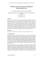
3. Multilayer perceptron artificial neural network (MPNN)
The structure of MPNN was introduced by Rumelhart (1986). It is one of the basic neural
network structures from which several others were derived.
The basic element of the MPNN is a neuron. Several neurons are organized into layers –
input, hidden (one or more) and output layer. Each neuron has a simple structure that
mimics the functionality of the neuron found in animals and the whole structure of layers
mimics the brain structure. This similarity gives rise to the name. Each neuron firstly
summarizes the weighted input values and then passes the sum through the transfer
function. If the transfer function is nonlinear, such as a basic sigmoid function or hyperbolic
tangent, then the whole structure acquires its great ability as an universal approximator.
The neurons in the input layer take the values from the model input variables and pass the
values to the neurons in the hidden layer, the hidden layer neurons pass the values to the
higher hidden layers and finally to the output layer that gives the model output value. The
output of each neuron is passed to the input of all neurons in the next higher layer. All the
connections between neurons are weighted. These interconnection weights are the basic
parameters of the model that are adjusted during the learning process.
Model inputs take their values from the input features – measured parameters that
determine the output of the model. Model output(s) represents the phenomenon that is
being reconstructed (approximated). Outputs are called output features.

www.intechopen.com

Artificial Neural Networks - a Useful Tool in Air Pollution and Meteorological Modelling

497
The values of one particular realization of all inputs is called the input vector, and the model
outputs values form the output vector. Both vectors together form a pattern. A pattern is
therefore like one dot in the multivariable space lying on the surface of the function the
model is approximating.
The whole idea of constructing a model to approximate a multivariable function is the
following: Firstly enough patterns should be available (for instance from the measurements)
with known input and output features. These patterns should be uniformly spread over the
whole investigated domain. Then the model topology is designed according to the number
of input and output features. The model learning stage consists of several adjustments of
model interconnection weights – in order to minimize the average error between the actual
measured output values and the output values that are produced by the neural network.
One of the algorithms that can be used for this purpose is the backpropagation algorithm. In
the process of learning the MPNN takes the information (about phenomenon under
investigation) that is available in the learning patterns and when learning is completed (the
model constructed) it can give the results for previously unknown patterns – where only
input values are presented to the network. This is possible if there were similar patterns (to
the unknown pattern) in the learning set. This is the so-called generalizing capability of the
MPNN. The similarity is mathematically speaking the distance between two patterns.
The basic rule of MPNN model construction is therefore to provide information rich
learning patterns.
There are some basic steps and methods that should be used in the model construction
process to obtain effective models. These steps will be summarized in the following
paragraphs and their practical use is shown in the exemplary applications that follow this
section.

f
f
f
f
b
2
b
S
b
1
c
S
u
1
u
2
u
3
u
R
. . .
. . .
. . .
. . .
. . .
. . .
INPUT LAYER HIDDEN LAYER OUTPUT LAYER
W
1,1
V

1
V
2
V
S
W
R,S
R NUMBER OF INPUTS
S NUMBER O F HIDDEN NODES
W WEIGHTS IN HIDDEN LAYER
b
I,J
I
BIASES IN HIDDEN LAYER
V WEIGHTS IN OUTPUT LAYER
c
I,J
I
BIASES IN OUTPUT LAYER

Fig. 1. The structure of a feedforward multilayer perceprtron neural network
www.intechopen.com

Advanced Air Pollution

498

f
b
1

u
1
u
2
u
3
u
R
. . .
. . .
. . .
INPUTS
NODE
(ARTIFICIAL NEURON
OR PERCEPTRON)
W
1
W
2
W
3
W
R
R NUMBER OF INPUTS

Fig. 2. Node (artificial neuron or perceptron)
3.1 Feature determination
Feature determination should be done in order to properly define the modelled domain
(independent variables), to enable all important information to be captured, to simplify
MPNN and therefore achieve more effective learning, to reduce the number of learning

patterns needed and to increase the probability of finding the global minimum of the error
function during learning.
Firstly the modeller should determine what the desired output of the model is. This can be
one or several parameters that can be measured or calculated. These are the output features.
For several output features it is usually more effective to establish one model for each
feature than one model for all. Then the input features should be determined from several
other measured parameters that represent the possible variables that cause or influence the
output parameter. Input features are the ones that have significant influence on the outputs.
Feature determination can be done heuristically (using expert knowledge about the
phenomenon under investigation) or using other methods (feature reduction that can be
extraction or selection (Devijver, 1982); examples of selection are contribution factors or
Saliency metrics techniques). In both the latter methods basically the model is firstly trained
with all available features and the higher absolute values of interconnection weights reveal
the more important input features.
It is extremely important that the feature determination process should not be based on a
linear method. Most of the processes in the atmosphere over complex terrain are not linearly
dependent on each other. Therefore if the input features are chosen from the possible input
measurements by a linear criterion (for instance calculation of the linear correlation factor
between the examined input measurement and output modelled parameter), then most
probably the important ones are rejected. An MPNN has the very important ability of being
able to simulate highly non-linear dependencies and the modeller should obtain the most
www.intechopen.com

Artificial Neural Networks - a Useful Tool in Air Pollution and Meteorological Modelling

499
advantage out of this. The above mentioned contribution factors and Saliency metrics
techniques both allow highly-nonlinear relationships to be found.
3.2 Model construction
The data base of the measurements (values of input and output features for several

situations – for instance for several measuring intervals) form the data base of patterns. It
should be divided into several sets (training, testing, production, on-line, remaining). The
training set is used to adjust the interconnection weights of the MPNN model. The testing
set is used periodically during the learning process to test the model’s generalizing
capabilities – this is optimization during learning. The final model is the one that gives the
best results on the testing set. In this way we prevent the model from becoming too
dependent on known patterns and therefore losing the generalizing capabilities. The
training and testing sets together form the learning set. A third set different from the
previous ones is the production set. This set is used for model verification to determine its
expected error. All three sets should have known input and output vectors. When the model
has been tained, it can be used on patterns with unknown output values. This set of patterns
is the on-line set – when a newly measured situation arises, the model gives us an answer.
3.3 Pattern selection
Only patterns with valuable information should be put into the learning set, while others are
rejected and form the remaining set. The pattern selection can be done either heuristically
or a Kohonen neural network can be used to sort patterns into groups and in this way the
KNN shows which ones are more important. The main goal of pattern selection techniques
is to select patterns over the whole of the modelled domain. These patterns should contain
all the information about the studied phenomenon. Patterns selected for the training and
testing set should represent all important but usually rare situations that may appear during
the further use of the model. Just having a lot of patterns that are the most common, but do
not represent the rare complicated situations, is certainly not enough for an effective model.
3.4 Network topology determination
The topology (number of neurons in the input, hidden and output layers) is determined
from the number of features and the number of patterns. Input and output features
determine the number of neurons in the input and output layers. The number of neurons in
the hidden layer(s) is usually determined as the number of inputs divided by two plus the
square root of the number of patterns. There is no rule for a perfect solution – the user
should acquire some experience.
3.5 Training and testing process

After the topology has been determined and the patterns prepared, a training algorithm (for
instance a backpropagation algorithm) should be used to determine the model’s
interconnection weights. Basically the algorithms have parameters that determine the speed
of learning. Learning is a process of finding the global minimum of the error function. If
during the learning process we move in big steps, the model cannot reach the bottom of the
minimum function, but escapes quickly to other local minima. If the steps are too small, the
model can be stuck in a local minimum far from the global one. During the learning process,
the network should be periodically tested on the testing set (not included in the training set)
www.intechopen.com

Advanced Air Pollution

500
to prevent overtraining. At the end the model is the network giving the best results on the
optimization – testing set. This is an optimizing process that finds the network with best
generalizing capabilities instead of the best memorizing capabilities. Learning speed
determination and optimization are usually far more important for successful learning than
having a slightly better or worse algorithm.
3.6 Model verification
When the model is trained, it should always be validated on the production set to determine
the expected error in further on-line use. To obtain a fair judgement of the model’s abilities,
the patterns that form the production set for validation should not be presented to the
model in the training or testing set at all.
The training, testing and production sets should reflect all the situations that can arise in the
on-line use of the model.
Feature determination and pattern selection are therefore the most crucial steps in model
construction and usually determine the model’s abilities.
4. Short term forecasting of ambient SO
2
concentrations using MPNN

First let us use the MPNN as a basis for short term ambient SO
2
concentration forecasting.
As an example for study the area around the Šoštanj Thermal Power Plant in Slovenia was
used. The studied domain of 30 by 30 km with the TPP in the centre lies in very complex
terrain – a basin surrounded by several hills that are cut by valleys. The area is characterized
by very low wind speeds, frequent calm situations and thermal inversions in winter that
cause severe air pollution. The whole of the studied area is covered by 6 ambient automatic
measuring stations (measuring basic meteorological parameters like wind, air temperature,
relative humidity and precipitation and pollutant concentrations) and emission stations in
the TPP. All the stations collect data every half hour.
The idea was to test the forecasting abilities of the new MPNN tool. Low winds and quick
wind changes in the area cause severe air pollution peaks of very short duration (only a few
intervals). We tried to establish a model that would forecast the SO
2
concentration for the
following half hour from the data available for present or past intervals (air pollution and
meteorological measurements). The task was a difficult one, because the work was
concentrated on rapid warning of short but severe SO
2
peaks and on not causing false alarms.
The data base of measurements was huge in all dimensions. There were over 50 parameters
that were measured every half hour and several years of data were available for analysis
(one year consists of over 17000 half hour intervals). It is obvious that all the data could not
be simply used together because of the computational space and time problems (this was at
the beginning of the PC era) and more importantly because the patterns with less
information would prevail over the sparse patterns carrying crucial information. The same
is valid for the different measured parameters that are the possible inputs to the model. This
huge data base forced us to establish methods for feature determination and pattern
selection. The idea was to find patterns that carry most of the available information and to

determine which measurements influence the modeled ambient SO
2
concentration at a
chosen station. It is very important to stress that we were seeking for highly non-linear
dependencies that the MPNN is able to model.
The whole procedure of feature determination and pattern selection techniques is explained
in detail in several our publications (Božnar, 1997; Mlakar, 1997; Mlakar & Božnar, 1996;
Božnar et. al, 1993; Božnar & Mlakar, 2001).
www.intechopen.com

Artificial Neural Networks - a Useful Tool in Air Pollution and Meteorological Modelling

501
This approach resulted in a model for a chosen station that used around 15 input
measurements from that and other stations to forecast the local SO
2
air pollution. The model
was trained with small (in comparison to the huge data base available) data sets of chosen
patterns. This resulted in a significant improvement of model forecasting ability.
It is also important that the usual cost functions (linear correlation coefficient, mean square
error, …) are not suitable for forecasting problems where most of the time nothing out of the
ordinary is happening, but when the peak of concentration comes, it is severe and short. It
was very easy to obtain very good values of the above mentioned cost functions – but this
does not tell anything about the real model capabilities (if it really correctly and on-time
predicts the coming SO
2
peak). Therefore we defined a new cost function termed p6
(Mlakar, 1997). This is the probability of successful forecasting of a high concentration
without causing false alarms. It is a very sharp cost function that clearly distinguishes good
models from the ones that are in the range of naive predictors.

In the process of SO
2
modelling it was clearly proven that feature determination and pattern
selection techniques influence the final model performance much more than the training
algorithms and other details of the establishment of the model. This is caused by the fact
that the information carried in the features and patterns of the available data set should be
presented to the model in the learning phase in a “model understandable” way. To
generalize this principle it can be stated that an understandable way is similar to a humanly
understandable way. People also cannot learn effectively if the informative and key
examples are hidden in large quantity of useless examples.
5. Daily ozone peak forecasting for a semi-urban area
A model for ozone forecasting was established for the city of Nova Gorica in Slovenia close to
the Adriatic sea (Grašič, 2006). During the hot summer period high ozone episodes are often
recorded. The idea of constructing the model is to have information about the ozone pollution
peak of the following day already available in the evening of the day before 19:00. That would
allow the population sensitive to ozone to plan their activities for the following day.
Slovene legislation defines warning values for a one hour average ozone concentration and
for eight hour moving average values. We concentrated our research on determination of
the maximum hourly value of ozone concentration of the following day. Ozone peaks
usually occur during the midday period, therefore the task deals with forecasting cca 17
hours in advance.
The available data were measurements from a local air pollution measuring station (SO
2
, O
3
,
NO, NO
2
, CO, VOC) that also measures ground level meteorological parameters (wind, air
temperature, relative humidity, air pressure and global solar radiation). In principle in the

evening meteorological forcasts are available for the city of Nova Gorica. Of these values
two are more reliable – the maximum daily air temperature and the average wind speed and
direction for the following midday. For the purpose of establishing the model from the
historical data base, actual measurements of these two parameters on the following days
were taken instead of prognostic values.
A two year data base was available for model construction and verification. In this case only
one pattern per day is available. Therefore two years data give cca 700 patterns only. Out of
this data base one winter and one summer month were excluded (were not used in the
learning process at all) for independent model verification.
Because of the small data base available for learning it was only divided into a randomly
taken group of 10% for testing (optimising) and the remaining 90% used for adjustment of
the model's weights (training). No other pattern selection was performed.
www.intechopen.com

Advanced Air Pollution

502
Feature selection was done in two steps. Firstly a wide selection of possible input features
was made using chemical knowledge about ozone formation and other related processes.
Then this wide range was narrowed using contribution factors. The finally selected input
features were air temperature, global solar radiation, NO, NO
2
, NO
x
, CO, O
3
all as 24h
average values calculated at 19:00 on the previous day, prognostic vector wind speed, sine
of wind direction and maximal hourly air temperature for the day of prediction (all three
prognostic values were taken from the available measured data base).

The verification of the model for approximately two months not used in the learning process
showed that the model has a good performance. For final judgement, a longer verification
period would be necessary. It is also expected that its performace would be slightly worse if
actual meteorological prognostic model predictions were taken instead of real
measurements (for the last three features).
6. Ground level wind reconstruction over complex terrain
Air pollution prediction was the first but not the only field where we successfully
constructed MPNN based models.
Recently we encountered the problem of missing ground level wind data on the location of a
planned industrial plant. The time available for the task was short and therefore it was not
possible to perform one year of measurements, and only 6 weeks of measurements were
available. The location was again in the complex terrain of Zasavje, Slovenia. Study of the
winds in the area clearly show that ground level wind reconstruction from global prognostic
meteorological models would not be useful because of the orographic complexity of the area.
But there are six existing meteorological stations in the area on sited from 2 to 10 km from
the planned location. None of these locations has the same characteristics as the new
location, so their data could not be used directly.
Our idea was to reconstruct one year of ground level wind data on the new location from
one year of wind data at the old station locations. This is a very suitable task for a MPNN
based model. The six weeks data base when wind measurements were available at both old
and new locations was used to train and verify the model.
In contrast to the SO2 forecasting problem, this problem again has a small data base consisting
of 6 weeks of half hour average values of wind speed and direction measurements at 7
locations. Therefore only the last week of measurements was reserved for final model
verification and was not used for model learning. The remaining five week data base was
again divided into a randomly taken 10% test set for optimization and 90% for training.
For every station vector and scalar half hour average values and maximum values of wind
speed were available, as well as wind direction. The vectors were also decomposed into
cosine and sine components. The decomposition into cosine and sine components is a trick
that should be used whenever we have a measurement of circular nature (such as azimuth

angle or hour within a day). All these measurements and their combination at the old
stations locations are candidates for model input features.
Firstly a heuristic feature selection was performed by simply comparing the similarity of
wind roses for the new and old locations. Then the final feature selection was repeated using
the contribution factors technique.
The results of the model verification show better results than expected, considering the high
complexity of the area studied.
The reconstructed wind speed mean absolute error at the new location was less than
0.4 m/s, the mean squared error 0.45 m/s and the linear correlation coefficient 0.84. The
www.intechopen.com

Artificial Neural Networks - a Useful Tool in Air Pollution and Meteorological Modelling

503
average absolute error for the wind direction was 35 degrees over the whole verification
data set (which contains a lot of very low wind speeds and calms) and as little as
15.5 degrees if only cases with a wind speed over 3 m/s were examined.
7. Other meteorological applications of MPNN
We successfully applied MPNN in the following meteorological problems that will be only
shortly explained:
• reconstruction of SODAR measurements,
• short term forecasting of ground level wind,
• reconstruction of diffuse solar radiation,
• correction of long wave solar radiation measurements.
7.1 Reconstruction of SODAR measurements
SODAR measurements are crucial for modern numerical Lagrangean particle models used
for short scale air pollution reconstruction over complex terrain. But SODAR measurements
are not always available. SO
2
air pollution was studied in detail (fourth chapter of this

article) in the Šoštanj area of Slovenia. In the Šoštanj basin SODAR measurements were
available only for an aproximately two month period during a measuring campaign (Elisei
et. al, 1992). The area of the basin and surrounding hills is well covered with ground level
wind measuring stations.
We made a MPNN based model to see whether it was possible to reconstruct SODAR upper
layer (not ground level) measurements from the measurements at other stations. A test
model was made for the level 50m above the ground. The results were quite good
(comparable to the Trbovlje wind reconstruction). Some details can be found in paper by
Božnar and Mlakar (1995).
7.2 Short term forecasting of ground level wind
In the same area around Šoštanj short term ground level wind forecasts would also be very
useful as an input to an SO
2
concentration forecasting model. Forecasts of wind changes for
the next few half hour intervals are more dependent on local thermal and solar radiation
changes than on the movement of global fronts. Due to terrain complexity again such
forecasts cannot be derived from regional prognostic meteorological models, because they
operate in too sparse (time and space) coordinates.
We constructed a model for ground level wind forecasting for one of the stations in the
Šoštanj region. The forecast was made for one averaging interval in advance. The input
features were ground level wind measurements from the studied station and from two other
stations for the current time interval. For wind speed one interval in the past was also used.
The results were very good for wind speed and acceptable for wind direction prediction.
Some details can be found in paper by Božnar and Mlakar (1995).
7.3 Reconstruction of diffuse solar radiation measurements and correction of long
wave solar radiation measurements
Our colleagues from Sao Paulo, Brazil made extensive research on the measurement of and
construction of correlation based models for diffuse solar radiation in the Sao Paulo urban
area (Oliveira et. al, 2002). The diffuse solar radiation component requires expensive
measuring procedures in comparison to other basic meteorological measurements,

www.intechopen.com

Advanced Air Pollution

504
including global and long wave solar radiation. Therefore it would be useful for many
purposes if the diffuse solar radiation component could be reconstructed from other simpler
meteorological measurements. An MPNN-based model was constructed for this purpose
that gives significantly better results than previously available models. Details can be found
in paper by Soares et. al, (2004).
Another problem arose from this work – correction of long wave measurements according
to the Fairall formula (Fairall et al, 1998). This correction requires additional measurements
of the temperature of the long wave sensor’s dome and base. There exist several years of
long wave solar radiation measurements for Sao Paulo but without the required additional
measurements for correction. We solved the problem by several months measurements of
the missing parameters and then establishing a MPNN-based model for reconstruction of
the Fairall correction from the basic meteorological measurements that are available for
several years (Oliveira, 2006). The model again gave very good results.
In both the above explained models, feature determination and pattern selection techniques
were applied in the model construction phase.
8. Kohonen neural network (KNN)
The Kohonen neural network (KNN) (Kohonen, 1995) differs significantly from the MPNN.
The main purpose of KNN is to sort multivariable patterns into groups (clusters) of similar
ones. It is important that the grouping criteria need not be known – therefore this is
unsupervised learning.
KNN is a very practical and effective tool for finding groups of similar patterns in data sets
where it is not known in advance (through some other available knowledge) what their
natural division into groups of similar patterns is.
The sorting principle is as follows: firstly the user prepares a data set of multivariable patterns
that should be searched for groups of similar ones. The pattern consists of input features (the

same definition as in MPNN). The output feature is the number of the cluster that the pattern
belongs to. The quantity of clusters should be determined by the user. The natural number of
clusters (the number of clusters that best fits the examined problem) cannot be determined
automatically. But there is a relatively simple way of finding it. The process of dividing data
set into groups is repeated for several different quantities of groups. For each division the
average standard deviation of the distance of all patterns from the corresponding centre of the
group should be calculated. On increasing the number of groups, the standard deviation
decreases rapidly until the natural number of groups is reached. After that, if we divide these
groups into more groups, the standard deviation decreases significantly slower than before.
Using this rule, the “natural” number of groups can be easily derived from a graph of the
average standard deviation of the distance versus the number of groups.
The crucial part of sorting is selection of the measure of distance appropriate to the problem
examined. In most cases the Euclidean distance between two vectors can be used. But it
should be noted that if the components of the vector represent measurements of different
natural processes, then each process should be normalized. If this is not done, some
components may prevail over others. Beside Euclidean distance, many other distance
measures that are known from pattern recognition theory can also be used.
In the iterative process when KNN sorts the available data set of patterns into a chosen
number of groups, it actually puts together patterns that are close one to another in terms of
the distance function used. The algorithm is again an iterative one and the user can stop the
process of division when the groups become stable.
www.intechopen.com

Artificial Neural Networks - a Useful Tool in Air Pollution and Meteorological Modelling

505

Fig. 3. Presentation of wind roses for all clusters for the division into 10 clusters
Feature determination is also an important process when using KNN. In this case feature
selection means that the user should find the inputs that can provide some information about

how a particular pattern differs from other ones. With KNN, feature determination is mostly
done heuristically according to the user’s knowledge about the examined phenomenon.
KNN is an extremely useful sorting tool for problems dealing with huge data bases and
multivariable patterns.
www.intechopen.com

Advanced Air Pollution

506
In the following paragraphs two successful problems that we solved using KNN will be
presented.
9. Sorting of ground level wind fields using KNN
The Šoštanj area (a basin in complex terrain, explained in previous sections) has very
colorful ground level wind field patterns due to the fact that the very low winds that prevail
there meander in the basin and follow the shape of nearby lying valleys and become
stronger over the hills and passes. Hence the wind roses of six ambient automatic measuring
stations (that were examined for SO
2
forecasting) look totally different, in spite of the fact
that they are only a few kilometers away one from another. This fact illustrates the
complexity of the ground level winds in the area.
We examined the following problem (Mlakar & Božnar, 1996): is it possible to find groups of
similar wind fields (a wind field in this case is represented by a packet of simultaneously
measured wind data at all stations) occurring in this area, or is the problem too stochastic to
be grouped? If there are groups, what is the “natural” number of groups there?
To answer these questions we examined the wind data for five stations. One station was
excluded because its location was inappropriate for representative wind measurements.
The data base of over 26000 half hour intervals was examined when wind measurements
were available for all five stations. Due to the complexity of the wind roses for the whole
data set it was expected that the natural number of groups would be very large. Several

divisions from 10 to 100 groups were tested. As a measure of division quality a special index
was defined – the weighted sum of the standard deviation of wind speed and the standard
deviation of wind direction within the obtained groups. The natural number of groups was
found to be around 32.
The quality of the division of the 26000 wind patterns into 32 groups was easily controlled
by plotting wind roses for the new groups for each station. The new wind roses were not
similar to the wind roses composed of the whole data set for each station. And also the wind
roses of different groups (and the pattern for five stations) were different one from another.
The pictures of the wind roses for 32 groups at five stations proved very obviously that the
sorting process was done in a very effective and successful way.
This example of wind data sorting is a very persuasive one to convince the user about the
effectiveness of KNN. This is due to the fact that wind roses are a graphical presentation
that can be easily comprehended and the differences or similarities visualized. And on the
other hand, there is no way (because of the area complexity) to do this sorting manually -
only on the basis of some meteorological knowledge.

10. KNN as a tool for pattern selection techniques for MPNN based models
Another very successful application where we used KNN was as a pattern selection
technique. When establishing methods for pattern selection that would not need user
knowledge about meteorological phenomenon, we used KNN to sort a huge data base of air
pollution patterns into natural groups of patterns. When the groups are obtained it is easy to
construct a training and testing set to effectively train the MPNN.
The method was developed for the case of SO
2
prediction in the Šoštanj area (Božnar, 1997).
The method of pattern selection using KNN showed the same improvement in the MPNN
model effectiveness as the method of using all the available detailed expert knowledge
www.intechopen.com

Artificial Neural Networks - a Useful Tool in Air Pollution and Meteorological Modelling

507
about air pollution in the area. Therefore KNN pattern selection techniques are particularly
suitable for problems where detailed expert knowledge is not available.
11. Conclusion
Two types of artificial neural networks were shown to be useful tools for environmental
modelling: the multilayer perceptron neural network MPNN and the Kohonen neural
network KNN. MPNN is an universal approximator. Therefore it can be used for modeling
phenomena where reconstruction or prediction of one (or several) parameters is required on
the basis of other measured parameters. In the model construction phase there are two
important steps that are often neglected. These are feature determination and pattern
selection techniques. The methods that we suggest can be used in very different
applications. They contribute much to the final model performance. Their contribution can
be described as extraction of useful information from the available data base of
measurements and presentation of this information to the neural network during the
learning process in the most plausible way. The variety of presented examples from air
pollution prediction to meteorological applications shows how flexible MPNN models can
be. Meteorological applications especially demonstrate that MPNN models can be a useful
additional tool in the field of meteorological preprocessors for modern air pollution models.
The variety of examples presented also proves that feature determination and pattern
selection techniques are more or less universal.
KNN is not used so widely as MPNN in atmospheric research. The examples presented here
prove that KNN is a very effective tool for sorting problems. It actually performs very well
also in cases where there is no a priori knowledge about similarities at all.
We hope that the given examples of successful use of artificial neural networks will inspire
other applications in atmospheric research.
12. Acknowledgment
The study was partially financed by the Slovenian Research Agency, Project No. L1-2082.
13. References
Božnar, M. (1997). Pattern selection strategies for a neural network - based short term air

pollution prediction model. Adeli, H. (ed.). Intelligent Information Systems IIS'97,
Grand Bahama Island, Bahamas, December 8-10, Proceedings. Los Alamitos,
California[etc.]: IEEE Computer Society, pp. 340-344
Božnar, M., Lesjak, M., & Mlakar, P. (1993). A neural network-based method for short-term
predictions of ambient SO2 concentrations in highly polluted industrial areas of
complex terrain. Atmospheric Environment, B 27(2), pp. 221-230.
Božnar, M. & Mlakar, P. (1995). Neural networks - a new mathematical tool for air pollution
modelling., Editors: Power, H., Moussiopoulos, N., Brebbia, C. A. Air pollution III.
Vol. 1, Air pollution theory and simulation. Southampton; Boston: Computational
Publications, pp. 259-266
Božnar, M. & Mlakar, P. (2001). Artificial neural network-based environmental models. Air
pollution modeling and its application XIV, Kluwer Academic: Plenum Publishers,
New York, pp. 483-490
www.intechopen.com

Advanced Air Pollution

508
Comrie, A.C. (1997). Comparing neural networks and resression models for ozone
forecasting. Journal of Air and Waste Management 47, pp. 653-663.
Devijver, J.K., (1982). Pattern recognition: A statistical Approach. Englewood Cliffs, Prentice-
Hall, Inc.
Elisei et. al (1992). Experimental Campaign for the Environmental Impact Evaluation of Sostanj
Thermal Power Plant, Progress Report, CISE, Milano
Fairall, C.W., Persson. P.O.G., Bradley, E.F., Payne, R.E., & Anderson, S.P. (1998). A New
Look at Calibration and Use of Eppley Precision Infrared Radiometers. Part I: Theory
and Application. Journal of Atmospheric and Oceanic Technology; 15, pp. 1229-1242
Gardner, M.W., & Dorling S.R. (1998). Artificial neural networks (the multilayer perceptron)
- a review of applications in the atmospheric sciences. Atmospheric Environment 32
(14/15), pp. 2627-2636.

Grašič, B., Mlakar, P., & Božnar, M. Z. (2006). Ozone prediction based on neural networks
and Gaussian processes. Il Nuovo Cimento C, Vol. 29, Issue 6, pp. 651-661
Hornik, K. (1991). Approximation capabilities of multilayer feedforward networks. Neural
Networks 4, pp. 251-257
Kohonen, T. (1995). Self-organizing maps. Springer, Berlin
Kurkova, V. (1992). Kolmogorov’s Theorem and Multilayer Neural Networks, Neural
Networks, 5, pp. 501-506
Lawrence, J. (1991). Introduction to Neural Networks, California Scientific Software, Grass Valley
Marzban, C., & Strumpf, G.J. (1996). A neural network for tornado prediction based on
doppler radar derivd attributes. Journal of Applied Meteorology 35, pp. 617-626
Mlakar, P. (1997). Determination of features for air pollution forecasting models. Adeli, H.
(ed.). Intelligent Information Systems IIS'97, Grand Bahama Island, Bahamas,
December -10, Proceedings. Los Alamitos, California, USA: IEEE Computer
Society 1997, pp. 350-354.
Mlakar, P. & Božnar, M. (1996). Analysis Of Winds And SO2 Concentrations In Complex
Terrain. Editors: Caussade, B., Power, H., Brebbia, C.A Air Pollution IV:
Monitoring, Simulation And Control. Southampton; Boston: Computational
Mechanics Publications, Cop., pp. 455-464.
Moseholm, L., Silva, J., & Larson, T. (1996). Forecasting carbon monoxide concentrations
near a sheltered intersection using video traffic surveillance and neural networks.
Transport Research 1D (1), pp. 15-28
Oliveira, A.P., Escobedo J.F., Machado A.J., & Soares J. (2002). Correlation models of diffuse
solar radiation applied to the City of São Paulo (Brazil). Applied Energy 71(1), pp. 59-
73.
Oliveira, A. P. De, Soares, J. R., Božnar, M., Mlakar, P., Escobedo, J. F. (2006). An application
of neural network technology to corrent the dome temperature effects on
pyrgeometer measurements. Journal of Atmospheric and Oceanic Technolog, vol. 23,
pp. 80-89.
Rumelhart, D.E., Hilton, G.E., Williams, R.J. (1986). Learning internal representation by error
propagation, in Parallel Distributed Processing: Explorations in the Nicrostructure of

Cognition. eds. DE Rumelhart and JL McClelland, Vol 1, MIT Press, Cambridge, MA
Soares, J., Oliveira, A.P., Božnar, M.Z., Mlakar, P., E
scobedo, J.F., & Machado, A.J., (2004).
Modeling hurly diffuse solar-radiation in the city of São Paulo using a
neural’network technique. Applied Energy 79(1), pp. 201-214.
Yi, J., & Prybutok, R. (1996). A neural network model forecasting for prediction of daily
maximum ozone concentration in an industrialised urban area. Environmental
Pollution 92 (3), pp. 349-357.
www.intechopen.com
Advanced Air Pollution
Edited by Dr. Farhad Nejadkoorki
ISBN 978-953-307-511-2
Hard cover, 584 pages
Publisher InTech
Published online 17, August, 2011
Published in print edition August, 2011
InTech Europe
University Campus STeP Ri
Slavka Krautzeka 83/A
51000 Rijeka, Croatia
Phone: +385 (51) 770 447
Fax: +385 (51) 686 166
www.intechopen.com
InTech China
Unit 405, Office Block, Hotel Equatorial Shanghai
No.65, Yan An Road (West), Shanghai, 200040, China
Phone: +86-21-62489820
Fax: +86-21-62489821
Leading air quality professionals describe different aspects of air pollution. The book presents information on
four broad areas of interest in the air pollution field; the air pollution monitoring; air quality modeling; the GIS

techniques to manage air quality; the new approaches to manage air quality. This book fulfills the need on the
latest concepts of air pollution science and provides comprehensive information on all relevant components
relating to air pollution issues in urban areas and industries. The book is suitable for a variety of scientists who
wish to follow application of the theory in practice in air pollution. Known for its broad case studies, the book
emphasizes an insightful of the connection between sources and control of air pollution, rather than being a
simple manual on the subject.
How to reference
In order to correctly reference this scholarly work, feel free to copy and paste the following:
Primož Mlakar and Marija Zlata Božnar (2011). Artificial Neural Networks - a Useful Tool in Air Pollution and
Meteorological Modelling, Advanced Air Pollution, Dr. Farhad Nejadkoorki (Ed.), ISBN: 978-953-307-511-2,
InTech, Available from: />useful-tool-in-air-pollution-and-meteorological-modelling