Brushless DC Motor Control Made Easy potx
Bạn đang xem bản rút gọn của tài liệu. Xem và tải ngay bản đầy đủ của tài liệu tại đây (573.48 KB, 48 trang )
2002 Microchip Technology Inc. DS00857A-page 1
AN857
INTRODUCTION
This application note discusses the steps of developing
several controllers for brushless motors. We cover sen-
sored, sensorless, open loop, and closed loop design.
There is even a controller with independent voltage and
speed controls so you can discover your motor’s char-
acteristics empirically.
The code in this application note was developed with
the Microchip PIC16F877 PICmicro
®
Microcontroller, in
conjuction with the In-Circuit Debugger (ICD). This
combination was chosen because the ICD is inexpen-
sive, and code can be debugged in the prototype hard-
ware without need for an extra programmer or
emulator. As the design develops, we program the tar-
get device and exercise the code directly from the
MPLAB
®
environment. The final code can then be
ported to one of the smaller, less expensive,
PICmicro microcontrollers. The porting takes minimal
effort because the instruction set is identical for all
PICmicro 14-bit core devices.
It should also be noted that the code was bench tested
and optimized for a Pittman N2311A011 brushless DC
motor. Other motors were also tested to assure that the
code was generally useful.
Anatomy of a BLDC
Figure 1 is a simplified illustration of BLDC motor con-
struction. A brushless motor is constructed with a per-
manent magnet rotor and wire wound stator poles.
Electrical energy is converted to mechanical energy by
the magnetic attractive forces between the permanent
magnet rotor and a rotating magnetic field induced in
the wound stator poles.
FIGURE 1: SIMPLIFIED BLDC MOTOR DIAGRAMS
Author: Ward Brown
Microchip Technology Inc.
N
S
A
C
a
a
b
b
c
c
B
com
com
com
N
N
S
S
110
010
011
101
100
001
N
S
S
N
6
3
4
1
2
5
A
C
B
c
b
a
com
Brushless DC Motor Control Made Easy
AN857
DS00857A-page 2 2002 Microchip Technology Inc.
In this example there are three electromagnetic circuits
connected at a common point. Each electromagnetic
circuit is split in the center, thereby permitting the per-
manent magnet rotor to move in the middle of the
induced magnetic field. Most BLDC motors have a
three-phase winding topology with star connection. A
motor with this topology is driven by energizing 2
phases at a time. The static alignment shown in
Figure 2, is that which would be realized by creating an
electric current flow from terminal A to B, noted as path
1 on the schematic in Figure 1. The rotor can be made
to rotate clockwise 60 degrees from the A to B align-
ment by changing the current path to flow from terminal
C to B, noted as path 2 on the schematic. The sug-
gested magnetic alignment is used only for illustration
purposes because it is easy to visualize. In practice,
maximum torque is obtained when the permanent mag-
net rotor is 90 degrees away from alignment with the
stator magnetic field.
The key to BLDC commutation is to sense the rotor
position, then energize the phases that will produce the
most amount of torque. The rotor travels 60 electrical
degrees per commutation step. The appropriate stator
current path is activated when the rotor is 120 degrees
from alignment with the corresponding stator magnetic
field, and then deactivated when the rotor is 60 degrees
from alignment, at which time the next circuit is acti-
vated and the process repeats. Commutation for the
rotor position, shown in Figure 1, would be at the com-
pletion of current path 2 and the beginning of current
path 3 for clockwise rotation. Commutating the electri-
cal connections through the six possible combinations,
numbered 1 through 6, at precisely the right moments
will pull the rotor through one electrical revolution.
In the simplified motor of Figure 1, one electrical revo-
lution is the same as one mechanical revolution. In
actual practice, BLDC motors have more than one of
the electrical circuits shown, wired in parallel to each
other, and a corresponding multi-pole permanent mag-
netic rotor. For two circuits there are two electrical rev-
olutions per mechanical revolution, so for a two circuit
motor, each electrical commutation phase would cover
30 degrees of mechanical rotation.
Sensored Commutation
The easiest way to know the correct moment to com-
mutate the winding currents is by means of a position
sensor. Many BLDC motor manufacturers supply
motors with a three-element Hall effect position sensor.
Each sensor element outputs a digital high level for 180
electrical degrees of electrical rotation, and a low level
for the other 180 electrical degrees. The three sensors
are offset from each other by 60 electrical degrees so
that each sensor output is in alignment with one of the
electromagnetic circuits. A timing diagram showing the
relationship between the sensor outputs and the
required motor drive voltages is shown in Figure 2.
FIGURE 2: SENSOR VERSUS DRIVE TIMING
A
+V
-V
Float
B
+V
-V
Float
C
+V
-V
Float
H
L
H
L
H
L
Sensor A
Sensor B
Sensor C
654321
6 1
Code
101 001 011
010 110 100
101 001
2002 Microchip Technology Inc. DS00857A-page 3
AN857
The numbers at the top of Figure 2 correspond to the
current phases shown in Figure 1. It is apparent from
Figure 2 that the three sensor outputs overlap in such
a way as to create six unique three-bit codes corre-
sponding to each of the drive phases. The numbers
shown around the peripheral of the motor diagram in
Figure 1 represent the sensor position code. The north
pole of the rotor points to the code that is output at that
rotor position. The numbers are the sensor logic levels
where the Most Significant bit is sensor C and the Least
Significant bit is sensor A.
Each drive phase consists of one motor terminal driven
high, one motor terminal driven low, and one motor ter-
minal left floating. A simplified drive circuit is shown in
Figure 3. Individual drive controls for the high and low
drivers permit high drive, low drive, and floating drive at
each motor terminal. One precaution that must be
taken with this type of driver circuit is that both high side
and low side drivers must never be activated at the
same time. Pull-up and pull-down resistors must be
placed at the driver inputs to ensure that the drivers are
off immediately after a microcontoller RESET, when the
microcontroller outputs are configured as high imped-
ance inputs.
Another precaution against both drivers being active at
the same time is called dead time control. When an out-
put transitions from the high drive state to the low drive
state, the proper amount of time for the high side driver
to turn off must be allowed to elapse before the low side
driver is activated. Drivers take more time to turn off
than to turn on, so extra time must be allowed to elapse
so that both drivers are not conducting at the same
time. Notice in Figure 3 that the high drive period and
low drive period of each output, is separated by a float-
ing drive phase period. This dead time is inherent to the
three phase BLDC drive scenario, so special timing for
dead time control is not necessary. The BLDC commu-
tation sequence will never switch the high-side device
and the low-side device in a phase, at the same time.
At this point we are ready to start building the motor
commutation control code. Commutation consists of
linking the input sensor state with the corresponding
drive state. This is best accomplished with a state table
and a table offset pointer. The sensor inputs will form
the table offset pointer, and the list of possible output
drive codes will form the state table. Code development
will be performed with a PIC16F877 in an ICD. I have
arbitrarily assigned PORTC as the motor drive port and
PORTE as the sensor input port. PORTC was chosen
as the driver port because the ICD demo board also
has LED indicators on that port so we can watch the
slow speed commutation drive signals without any
external test equipment.
Each driver requires two pins, one for high drive and
one for low drive, so six pins of PORTC will be used to
control the six motor drive MOSFETS. Each sensor
requires one pin, so three pins of PORTE will be used
to read the current state of the motor’s three-output
sensor. The sensor state will be linked to the drive state
by using the sensor input code as a binary offset to the
drive table index. The sensor states and motor drive
states from Figure 2 are tabulated in Table 1.
FIGURE 3: THREE PHASE BRIDGE
To A
-V
M
+V
M
A High
control
A Low
control
To B
-V
M
+V
M
B High
control
B Low
control
To C
-V
M
+V
M
C High
control
C Low
control
AN857
DS00857A-page 4 2002 Microchip Technology Inc.
TABLE 1: CW SENSOR AND DRIVE BITS BY PHASE ORDER
Sorting Table 1 by sensor code binary weight results in Table 2. Activating the motor drivers, according to a state table
built from Table 2, will cause the motor of Figure 1 to rotate clockwise.
TABLE 2: CW SENSOR AND DRIVE BITS BY SENSOR ORDER
Counter clockwise rotation is accomplished by driving current through the motor coils in the direction opposite of that
for clockwise rotation. Table 3 was constructed by swapping all the high and low drives of Table 2. Activating the motor
coils, according to a state table built from Table 3, will cause the motor to rotate counter clockwise. Phase numbers in
Table 3 are preceded by a slash denoting that the EMF is opposite that of the phases in Table 2.
TABLE 3: CCW SENSOR AND DRIVE BITS
The code segment for determining the appropriate drive word from the sensor inputs is shown in Figure 4.
Pin RE2 RE1 RE0 RC5 RC4 RC3 RC2 RC1 RC0
Phase
Sensor
C
Sensor
B
Sensor
A
C High
Drive
C Low
Drive
B High
Drive
B Low
Drive
A High
Drive
A Low
Drive
1 101000110
2 100100100
3 110100001
4 010001001
5 011011000
6 001010010
Pin RE2 RE1 RE0 RC5 RC4 RC3 RC2 RC1 RC0
Phase
Sensor
C
Sensor
B
Sensor
A
C High
Drive
C Low
Drive
B High
Drive
B Low
Drive
A High
Drive
A Low
Drive
6 001010010
4 010001001
5 011011000
2 100100100
1 101000110
3 110100001
Pin RE2 RE1 RE0 RC5 RC4 RC3 RC2 RC1 RC0
Phase
Sensor
C
Sensor
B
Sensor
A
C High
Drive
C Low
Drive
B High
Drive
B Low
Drive
A High
Drive
A Low
Drive
/6 001100001
/4 010000110
/5 011100100
/2 100011000
/1 101001001
/3 110010010
2002 Microchip Technology Inc. DS00857A-page 5
AN857
FIGURE 4: COMMUTATION CODE SEGMENT
#define DrivePort PORTC
#define SensorMask B’00000111’
#define SensorPort PORTE
#define DirectionBit PORTA, 1
Commutate
movlw SensorMask ;retain only the sensor bits
andwf SensorPort ;get sensor data
xorwf LastSensor, w ;test if motion sensed
btfsc STATUS, Z ;zero if no change
return ;no change - return
xorwf LastSensor, f ;replace last sensor data with current
btfss DirectionBit ;test direction bit
goto FwdCom ;bit is zero - do forward commutation
;reverse commutation
movlw HIGH RevTable ;get MS byte to table
movwf PCLATH ;prepare for computed GOTO
movlw LOW RevTable ;get LS byte of table
goto Com2
FwdCom ;forward commutation
movlw HIGH FwdTable ;get MS byte of table
movwf PCLATH ;prepare for computed GOTO
movlw LOW FwdTable ;get LS byte of table
Com2
addwf LastSensor, w ;add sensor offset
btfsc STATUS, C ;page change in table?
incf PCLATH, f ;yes - adjust MS byte
call GetDrive ;get drive word from table
movwf DriveWord ;save as current drive word
return
GetDrive
movwf PCL
FwdTable
retlw B’00000000’ ;invalid
retlw B’00010010’ ;phase 6
retlw B’00001001’ ;phase 4
retlw B’00011000’ ;phase 5
retlw B’00100100’ ;phase 2
retlw B’00000110’ ;phase 1
retlw B’00100001’ ;phase 3
retlw B’00000000’ ;invalid
RevTable
retlw B’00000000’ ;invalid
retlw B’00100001’ ;phase /6
retlw B’00000110’ ;phase /4
retlw B’00100100’ ;phase /5
retlw B’00011000’ ;phase /2
retlw B’00001001’ ;phase /1
retlw B’00010010’ ;phase /3
retlw B’00000000’ ;invalid
AN857
DS00857A-page 6 2002 Microchip Technology Inc.
Before we try the commutation code with our motor, lets
consider what happens when a voltage is applied to a
DC motor. A greatly simplified electrical model of a DC
motor is shown in Figure 5.
FIGURE 5: DC MOTOR EQUIVALENT
CIRCUIT
When the rotor is stationary, the only resistance to cur-
rent flow is the impedance of the electromagnetic coils.
The impedance is comprised of the parasitic resistance
of the copper in the windings, and the parasitic induc-
tance of the windings themselves. The resistance and
inductance are very small by design, so start-up cur-
rents would be very large, if not limited.
When the motor is spinning, the permanent magnet
rotor moving past the stator coils induces an electrical
potential in the coils called Back Electromotive Force,
or BEMF. BEMF is directly proportional to the motor
speed and is determined from the motor voltage con-
stant K
V
.
EQUATION 1:
In an ideal motor, R and L are zero, and the motor will
spin at a rate such that the BEMF exactly equals the
applied voltage.
The current that a motor draws is directly proportional
to the torque load on the motor shaft. Motor current is
determined from the motor torque constant K
T
.
EQUATION 2:
An interesting fact about K
T
and K
V
is that their product
is the same for all motors. Volts and Amps are
expressed in MKS units, so if we also express K
T
in
MKS units, that is N-M/Rad/Sec, then the product of K
V
and K
T
is 1.
EQUATION 3:
This is not surprising when you consider that the units
of the product are [1/(V*A)]*[(N*M)/(Rad/Sec)], which is
the same as mechanical power divided by electrical
power.
If voltage were to be applied to an ideal motor from an
ideal voltage source, it would draw an infinite amount of
current and accelerate instantly to the speed dictated
by the applied voltage and K
V
. Of course no motor is
ideal, and the start-up current will be limited by the par-
asitic resistance and inductance of the motor windings,
as well as the current capacity of the power source.
Two detrimental effects of unlimited start-up current
and voltage are excessive torque and excessive cur-
rent. Excessive torque can cause gears to strip, shaft
couplings to slip, and other undesirable mechanical
problems. Excessive current can cause driver MOS-
FETS to blow out and circuitry to burn.
We can minimize the effects of excessive current and
torque by limiting the applied voltage at start-up with
pulse width modulation (PWM). Pulse width modulation
is effective and fairly simple to do. Two things to con-
sider with PWM are, the MOSFET losses due to switch-
ing, and the effect that the PWM rate has on the motor.
Higher PWM frequencies mean higher switching
losses, but too low of a PWM frequency will mean that
the current to the motor will be a series of high current
pulses instead of the desired average of the voltage
waveform. Averaging is easier to attain at lower fre-
quencies if the parasitic motor inductance is relatively
high, but high inductance is an undesirable motor char-
acteristic. The ideal frequency is dependent on the
characteristics of your motor and power switches. For
this application, the PWM frequency will be approxi-
mately 10 kHz.
BEMF
Motor
R
L
RPM = K
V
x Volts
BEMF = RPM / K
V
Torque = K
T
x Amps
K
V
* K
T
= 1
2002 Microchip Technology Inc. DS00857A-page 7
AN857
We are using PWM to control start-up current, so why
not use it as a speed control also? We will use the ana-
log-to-digital converter (ADC), of the PIC16F877 to
read a potentiometer and use the voltage reading as
the relative speed control input. Only 8 bits of the ADC
are used, so our speed control will have 256 levels. We
want the relative speed to correspond to the relative
potentiometer position. Motor speed is directly propor-
tional to applied voltage, so varying the PWM duty
cycle linearly from 0% to 100% will result in a linear
speed control from 0% to 100% of maximum RPM.
Pulse width is determined by continuously adding the
ADC result to the free running Timer0 count to deter-
mine when the drivers should be on or off. If the addi-
tion results in an overflow, then the drivers are on,
otherwise they are off. An 8-bit timer is used so that the
ADC to timer additions need no scaling to cover the full
range. To obtain a PWM frequency of 10 kHz Timer0
must be running at 256 times that rate, or 2.56 MHz.
The minimum prescale value for Timer0 is 1:2, so we
need an input frequency of 5.12 MHz. The input to
Timer0 is F
OSC/4. This requires an FOSC of 20.48 MHz.
That is an odd frequency, and 20 MHz is close enough,
so we will use 20 MHz resulting in a PWM frequency of
9.77 kHz.
There are several ways to modulate the motor drivers.
We could switch the high and low side drivers together,
or just the high or low driver while leaving the other
driver on. Some high side MOSFET drivers use a
capacitor charge pump to boost the gate drive above
the drain voltage. The charge pump charges when the
driver is off and discharges into the MOSFET gate
when the driver is on. It makes sense then to switch the
high side driver to keep the charge pump refreshed.
Even though this application does not use the charge
pump type drivers, we will modulate the high side driver
while leaving the low side driver on. There are three
high side drivers, any one of which could be active
depending on the position of the rotor. The motor drive
word is 6-bits wide, so if we logically AND the drive
word with zeros in the high driver bit positions, and 1’s
in the low driver bit positions, we will turn off the active
high driver regardless which one of the three it is.
We have now identified 4 tasks of the control loop:
• Read the sensor inputs
• Commutate the motor drive connections
• Read the speed control ADC
• PWM the motor drivers using the ADC and Timer0
addition results
At 20 MHz clock rate, control latency, caused by the
loop time, is not significant so we will construct a simple
polled task loop. The control loop flow chart is shown in
Figure 6 and code listings are in Appendix B.
AN857
DS00857A-page 8 2002 Microchip Technology Inc.
FIGURE 6: SENSORED DRIVE FLOWCHART
Initialize
ADC
Ready
?
Read new ADC
Set ADC GO
Add ADRESH to
TMR0
Carry?
Mask Drive
Word
Output Drive
Word
Sensor
Change
Save Sensor
Code
Commutate
Yes
No
No
Yes
No
Yes
2002 Microchip Technology Inc. DS00857A-page 9
AN857
Sensorless Motor Control
It is possible to determine when to commutate the
motor drive voltages by sensing the back EMF voltage
on an undriven motor terminal during one of the drive
phases. The obvious cost advantage of sensorless
control is the elimination of the Hall position sensors.
There are several disadvantages to sensorless control:
• The motor must be moving at a minimum rate to
generate sufficient back EMF to be sensed
• Abrupt changes to the motor load can cause the
BEMF drive loop to go out of lock
• The BEMF voltage can be measured only when
the motor speed is within a limited range of the
ideal commutation rate for the applied voltage
• Commutation at rates faster than the ideal rate
will result in a discontinuous motor response
If low cost is a primary concern and low speed motor
operation is not a requirement and the motor load is not
expected to change rapidly then sensorless control
may be the better choice for your application.
Determining the BEMF
The BEMF, relative to the coil common connection
point, generated by each of the motor coils, can be
expressed as shown in Equation 4 through Equation 6.
EQUATION 4:
EQUATION 5:
EQUATION 6:
FIGURE 7: BEMF EQUIVALENT
CIRCUIT
Figure 7 shows the equivalent circuit of the motor with
coils B and C driven while coil A is undriven and avail-
able for BEMF measurement. At the commutation fre-
quency the L's are negligible. The R's are assumed to
be equal. The L and R components are not shown in
the A branch since no significant current flows in this
part of the circuit so those components can be ignored.
B
BEMF
= sin (
α )
2
π
3
C
BEMF
= sin
α
-
—
4π
3
A
BEMF
= sin α - —
B
BEMF
C
BEMF
A
BEMF
V
R
L
R
L
COM
A
B
C
AN857
DS00857A-page 10 2002 Microchip Technology Inc.
The BEMF generated by the B and C coils in tandem,
as shown in Figure 7, can be expressed as shown in
Equation 7.
EQUATION 7:
The sign reversal of
C
BEMF
is due to moving the refer-
ence point from the common connection to ground.
Recall that there are six drive phases in one electrical
revolution. Each drive phase occurs +/- 30 degrees
around the peak back EMF of the two motor windings
being driven during that phase. At full speed the
applied DC voltage is equivalent to the RMS BEMF
voltage in that 60 degree range. In terms of the peak
BEMF generated by any one winding, the RMS BEMF
voltage across two of the windings can be expressed
as shown in Equation 8.
EQUATION 8:
We will use this result to normalize the BEMF diagrams
presented later, but first lets consider the expected
BEMF at the undriven motor terminal.
Since the applied voltage is pulse width modulated, the
drive alternates between on and off throughout the
phase time. The BEMF, relative to ground, seen at the
A terminal when the drive is on, can be expressed as
shown in Equation 9.
EQUATION 9:
Notice that the winding resistance cancels out, so
resistive voltage drop, due to motor torque load, is not
a factor when measuring BEMF.
The BEMF, relative to ground, seen at the A terminal
when the drive is off can be expressed as shown in
Equation 10.
EQUATION 10:
BEMF
BC
= B
BEMF
- C
BEMF
BEMF
RMS
= — ∫ sin (α) - sin α - — dα
3
π
π
2
π
6
2
BEMF
RMS
= +
3
π
π
2
π
3
4
BEMF
RMS
= 1.6554
2π
3
BEMF
A
=
[
V -
(
B
BEMF
- C
BEMF
)]
R
C + A
BEMF
BEMF
BEMF
A
=
V - B
BEMF
+ C
BEMF
C
BEMF
+ A
BEMF
2
R
2
-
-
BEMF
A
= A
BEMF
- C
BEMF
2002 Microchip Technology Inc. DS00857A-page 11
AN857
Figure 8 is a graphical representation of the BEMF for-
mulas computed over one electrical revolution. To
avoid clutter, only the terminal A waveform, as would
be observed on a oscilloscope is displayed and is
denoted as BEMF(drive on). The terminal A waveform
is flattened at the top and bottom because at those
points the terminal is connected to the drive voltage or
ground. The sinusoidal waveforms are the individual
coil BEMFs relative to the coil common connection
point. The 60 degree sinusoidal humps are the BEMFs
of the driven coil pairs relative to ground. The entire
graph has been normalized to the RMS value of the coil
pair BEMFs.
FIGURE 8: BEMF AT 100% DRIVE
Notice that the BEMF(drive on) waveform is fairly linear
and passes through a voltage that is exactly half of the
applied voltage at precisely 60 degrees which coin-
cides with the zero crossing of the coil A BEMF wave-
form. This implies that we can determine the rotor
electrical position by detecting when the open terminal
voltage equals half the applied voltage.
What happens when the PWM duty cycle is less than
100%? Figure 9 is a graphical representation of the
BEMF formulas computed over one electrical revolu-
tion when the effective applied voltage is 50% of that
shown in Figure 8. The entire graph has been normal-
ized to the peak applied voltage.
BLDC Motor Waveforms
-1
-0.5
0
0.5
1
1.5
-30 30 90 150 210 270 330
Electrical Degrees
Vollts (Normalized to DC Drive)
B
C
A
ABS(B-C)
ABS(C-A)
ABS(A-B)
BEMF(drive on)
(PWM at 100% Duty Cycle)
AN857
DS00857A-page 12 2002 Microchip Technology Inc.
FIGURE 9: BEMF AT 50% DRIVE
As expected the BEMF waveforms are all reduced pro-
portionally but notice that the BEMF on the open termi-
nal still equals half the applied voltage midway through
the 60 degree drive phase. This occurs only when the
drive voltage is on. Figure 10 shows a detail of the open
terminal BEMF when the drive voltage is on and when
the drive voltage is off. At various duty cycles, notice
that the drive on curve always equals half the applied
voltage at 60 degrees.
BLDC Motor Waveforms
-1
-0.5
0
0.5
1
1.5
-30 30 90 150 210 270 330
Electrical Degrees
Vollts (Normalized to DC Drive)
B
C
A
ABS(B-C)
ABS(C-A)
ABS(A-B)
BEMF(drive on)
(PWM at 50% Duty Cycle)
2002 Microchip Technology Inc. DS00857A-page 13
AN857
FIGURE 10: DRIVE ON VS. DRIVE OFF BEMF
How well do the predictions match an actual motor?
Figure 11 is shows the waveforms present on terminal
A of a Pittman N2311A011 brushless motor at various
PWM duty cycle configurations. The large transients,
especially prevalent in the 100% duty cycle waveform,
are due to flyback currents caused by the motor wind-
ing inductance.
Floating Terminal Back EMF
0
0.5
1
30 90
Electrical Degrees
Voltage (Normalized to DC Drive)
BEMF(drive on)
BEMF(drive off)
(PWM at 100% Duty Cycle)
Floating Terminal Back EMF
0
0.5
1
30 90
Electrical Degrees
Voltage (Normalized to DC Drive)
BEMF(drive on)
BEMF(drive off)
(PWM at 60% Duty Cycle)
Floating Terminal Back EMF
0
0.5
1
30 90
Electrical Degrees
Voltage (Normalized to DC Drive)
BEMF(drive on)
BEMF(drive off)
(PWM at 75% Duty Cycle)
Floating Terminal Back EMF
0
0.5
1
30 90
Electrical Degrees
Voltage (Normalized to DC Drive)
BEMF(drive on)
BEMF(drive off)
(PWM at 10% Duty Cycle)
AN857
DS00857A-page 14 2002 Microchip Technology Inc.
FIGURE 11: PITTMAN BEMF WAVEFORMS
The rotor position can be determined by measuring the
voltage on the open terminal when the drive voltage is
applied and then comparing the result to one half of the
applied voltage.
Recall that motor speed is proportional to the applied
voltage. The formulas and graphs presented so far rep-
resent motor operation when commutation rate coin-
cides with the effective applied voltage. When the
commutation rate is too fast then commutation occurs
early and the zero crossing point occurs later in the
drive phase. When the commutation rate is too slow
then commutation occurs late and the zero crossing
point occurs earlier in the drive phase. We can sense
and use this shift in zero crossing to adjust the commu-
tation rate to keep the motor running at the ideal speed
for the applied voltage and load torque.
100% Duty Cycle 50% Duty Cycle
10% Duty Cycle75% Duty Cycle
2002 Microchip Technology Inc. DS00857A-page 15
AN857
Open Loop Speed Control
An interesting property of brushless DC motors is that
they will operate synchronously to a certain extent. This
means that for a given load, applied voltage, and com-
mutation rate the motor will maintain open loop lock
with the commutation rate provided that these three
variables do not deviate from the ideal by a significant
amount. The ideal is determined by the motor voltage
and torque constants. How does this work? Consider
that when the commutation rate is too slow for an
applied voltage, the BEMF will be too low resulting in
more motor current. The motor will react by accelerat-
ing to the next phase position then slow down waiting
for the next commutation. In the extreme case the
motor will snap to each position like a stepper motor
until the next commutation occurs. Since the motor is
able to accelerate faster than the commutation rate,
rates much slower than the ideal can be tolerated with-
out losing lock but at the expense of excessive current.
Now consider what happens when commutation is too
fast. When commutation occurs early the BEMF has
not reached peak resulting in more motor current and a
greater rate of acceleration to the next phase but it will
arrive there too late. The motor tries to keep up with the
commutation but at the expense of excessive current.
If the commutation arrives so early that the motor can
not accelerate fast enough to catch the next commuta-
tion, lock is lost and the motor spins down. This hap-
pens abruptly not very far from the ideal rate. The
abrupt loss of lock looks like a discontinuity in the motor
response which makes closed loop control difficult. An
alternative to closed loop control is to adjust the com-
mutation rate until self locking open loop control is
achieved. This is the method we will use in our applica-
tion.
When the load on a motor is constant over it’s operating
range then the response curve of motor speed relative
to applied voltage is linear. If the supply voltage is well
regulated, in addition to a constant torque load, then
the motor can be operated open loop over it’s entire
speed range. Consider that with pulse width modula-
tion the effective voltage is linearly proportional to the
PWM duty cycle. An open loop controller can be made
by linking the PWM duty cycle to a table of motor speed
values stored as the time of commutation for each drive
phase. We need a table because revolutions per unit
time is linear, but we need time per revolution which is
not linear. Looking up the time values in a table is much
faster than computing them repeatedly.
The program that we use to run the motor open loop is
the same program we will use to automatically adjust
the commutation rate in response to variations in the
torque load. The program uses two potentiometers as
speed control inputs. One potentiometer, we’ll call it the
PWM potentiometer, is directly linked to both the PWM
duty cycle and the commutation time lookup table. The
second potentiometer, we’ll call this the Offset potenti-
ometer, is used to provide an offset to the PWM duty
cycle determined by the PWM potentiometer. An ana-
log-to-digital conversion of the PWM potentiometer
produces a number between 0 and 255. The PWM duty
cycle is generated by adding the PWM potentiometer
reading to a free running 8-bit timer. When the addition
results in a carry the drive state is on, otherwise it is off.
The PWM potentiometer reading is also used to access
the 256 location commutation time lookup table. The
Offset potentiometer also produces a number between
0 and 255. The Most Significant bit of this number is
inverted making it a signed number between -128 and
127. This offset result, when added to the PWM poten-
tiometer, becomes the PWM duty cycle threshold, and
controls the drive on and off states described previ-
ously.
Closed Loop Speed Control
Closed loop speed control is achieved by unlinking the
commutation time table index from the PWM duty cycle
number. The PWM potentiometer is added to a fixed
manual threshold number between 0 and 255. When
this addition results in a carry, the mode is switched to
automatic. On entering Automatic mode the commuta-
tion index is initially set to the PWM potentiometer
reading. Thereafter, as long as Automatic mode is still
in effect, the commutation table index is automatically
adjusted up or down according to voltages read at
motor terminal A at specific times. Three voltage read-
ings are taken.
FIGURE 12: BEMF SAMPLE TIMES
AN857
DS00857A-page 16 2002 Microchip Technology Inc.
The first reading is taken during drive phase 4 when ter-
minal A is actively driven high. This is the applied volt-
age. The next two readings are taken during drive
phase 5 when terminal A is floating. The first reading is
taken when ¼ of the commutation time has elapsed
and the second reading is taken when ¾ of the commu-
tation time has elapsed. We'll call these readings 1 and
2 respectively. The commutation table index is adjusted
according to the following relationship between the
applied voltage reading and readings 1 and 2:
• Index is unchanged if Reading 1 > Applied Volt-
age/2 and Reading 2 < Applied Voltage/2
• Index is increased if Reading 1 < Applied Voltage/
2
• Index is decreased if Reading 1 > Applied Volt-
age/2 and Reading 2 > Applied Voltage/2
The motor rotor and everything it is connected to has a
certain amount of inertia. The inertia delays the motor
response to changes in voltage load and commutation
time. Updates to the commutation time table index are
delayed to compensate for the mechanical delay and
allow the motor to catch up.
Acceleration and Deceleration Delay
The inertia of the motor and what it is driving, tends to
delay motor response to changes in the drive voltage.
We need to compensate for this delay by adding a
matching delay to the control loop. The control loop
delay requires two time constants, a relatively slow one
for acceleration, and a relatively fast one for decelera-
tion.
Consider what happens in the control loop when the
voltage to the motor suddenly rises, or the motor load
is suddenly reduced. The control senses that the motor
rotation is too slow and attempts to adjust by making
the commutation time shorter. Without delay in the con-
trol loop, the next speed measurement will be taken
before the motor has reacted to the adjustment, and
another speed adjustment will be made. Adjustments
continue to be made ahead of the motor response until
eventually, the commutation time is too short for the
applied voltage, and the motor goes out of lock. The
acceleration timer delay prevents this runaway condi-
tion. Since the motor can tolerate commutation times
that are too long, but not commutation times that are
too short, the acceleration time delay can be longer
than required without serious detrimental effect.
Consider what happens in the control loop when the
voltage to the motor suddenly falls, or the motor load is
suddenly increased. If the change is sufficiently large,
commutation time will immediately be running too short
for the motor conditions. The motor cannot tolerate this,
and loss of lock will occur. To prevent loss of lock, the
loop deceleration timer delay must be short enough for
the control loop to track, or precede the changing motor
condition. If the time delay is too short, then the control
loop will continue to lengthen the commutation time
ahead of the motor response resulting in over compen-
sation. The motor will eventually slow to a speed that
will indicate to the BEMF sensor that the speed is too
slow for the applied voltage. At that point, commutation
deceleration will cease, and the commutation change
will adjust in the opposite direction governed by the
acceleration time delay. Over compensation during
deceleration will not result in loss of lock, but will cause
increased levels of torque ripple and motor current until
the ideal commutation time is eventually reached.
Determining The Commutation Time
Table Values
The assembler supplied with MPLAB performs all cal-
culations as 32-bit integers. To avoid the rounding
errors that would be caused by integer math, we will
use a spreadsheet, such as Excel, to compute the table
entries then cut and paste the results to an include file.
The spreadsheet is setup as shown in Table 4.
TABLE 4: COMMUTATION TIME TABLE VALUES
Variable Name Number or Formula Description
Phases 12 Number of commutation phase changes in one
mechanical revolution.
FOSC 20 MHz Microcontroller clock frequency
F
OSC_4 FOSC/4 Microcontroller timers source clock
Prescale 4 Timer 1 prescale
MaxRPM 8000 Maximum expected speed of the motor at full
applied voltage
MinRPM (60*F
OSC_4)/Phases*Prescale*65535)+1 Limitation of 16-bit timer
Offset -345 This is the zero voltage intercept on the RPM axis.
A property normalized to the 8-bit A to D converter.
Slope (MaxRPM-Offset)/255 Slope of the RPM to voltage input response curve
normalized to the 8-bit A to D converter.
2002 Microchip Technology Inc. DS00857A-page 17
AN857
The body of the spreadsheet starts arbitrarily at row 13.
Row 12 contains the column headings. The body of the
spreadsheet is constructed as follows:
• Column A is the commutation table index number
N. The numbers in column A are integers from 0
to 255.
• Column B is the RPM that will result by using the
counter values at index number N. The formula in
column B is: =IF(Offset+A13*Slope>MinRPM,Off-
set+A13*Slope,MinRPM).
• Column C is the duration of each commutation
phase expressed in seconds. The formula for col-
umn C is: =60/(Phases*B13).
• Column D is the duration of each commutation
phase expressed in timer counts. The formula for
column D is: =C13*F
OSC_4/Prescale.
The range of commutation phase times at a reasonable
resolution requires a 16-bit timer. The timer counts from
0 to a compare value then automatically resets to 0.
The compare values are stored in the commutation
time table. Since the comparison is 16 bits and tables
can only handle 8 bits the commutation times will be
stored in two tables accessed by the same index.
• Column E is the most significant byte of the 16-bit
timer compare value. The formula for column E is:
=CONCATENATE("retlw high D'”,INT(D13),”'”).
• Column F is the least significant byte of the 16-bit
timer compare value. The formula for column F is:
=CONCATENATE(“retlw low D'”,INT(D13),”'”).
When all spreadsheet formulas have been entered in
row 13, the formulas can be dragged down to row 268
to expand the table to the required 256 entries. Col-
umns E and F will have the table entries in assembler
ready format. An example of the table spreadsheet is
shown in Figure 13.
FIGURE 13: PWM LOOKUP TABLE GENERATOR
AN857
DS00857A-page 18 2002 Microchip Technology Inc.
Using Open Loop Control to Determine
Motor Characteristics
You can measure the motor characteristics by operat-
ing the motor in Open Loop mode, and measuring the
motor current at several applied voltages. You can then
chart the response curve in a spreadsheet, such as
Excel, to determine the slope and offset numbers.
Finally, plug the maximum RPM and offset numbers
back into the table generator spreadsheet to regener-
ate the RPM tables.
To operate the motor in Open Loop mode:
• Set the manual threshold number (ManThresh)
to 0xFF. This will prevent the Auto mode from tak-
ing over.
• When operating the motor in Open Loop mode,
start by adjusting the offset control until the motor
starts to move. You may also need to adjust the
PWM control slightly above minimum.
• After the motor starts, you can increase the PWM
control to increase the motor speed. The RPM
and voltage will track, but you will need to adjust
the offset frequently to optimize the voltage for the
selected RPM.
• Optimize the voltage by adjusting the offset for
minimum current.
To obtain the response offset with Excel
®
, enter the
voltage (left column), and RPM (right column) pairs in
adjacent columns of the spreadsheet. Use the chart
wizard to make an X-Y scatter chart. When the chart is
finished, right click on the response curve and select
the pop-up menu “add trendline. . .” option. Choose the
linear regression type and, in the Options tab, check
the “display equation on chart” option. An example of
the spreadsheet is shown in Figure 14.
FIGURE 14: MOTOR RESPONSE SCOPE DETERMINATION
2002 Microchip Technology Inc. DS00857A-page 19
AN857
Constructing The Sensorless Control
Code
At this point we have all the pieces required to control
a sensorless motor. We can measure BEMF and the
applied voltage then compare them to each other to
determine rotor position. We can vary the effective
applied voltage with PWM and control the speed of the
motor by timing the commutation phases. Some mea-
surement events must be precisely timed. Other mea-
surement events need not to interfere with each other.
The ADC must be switched from one source to another
and allow for sufficient acquisition time. Some events
must happen rapidly with minimum latency. These
include PWM and commutation.
We can accomplish everything with a short main loop
that calls a state table. The main loop will handle PWM
and commutation and the state table will schedule
reading the two potentiometers, the peak applied volt-
age and the BEMF voltages at two times when the
attached motor terminal is floating. Figure A-1 through
Figure A-10, in Appendix A, is the resulting flow chart
of sensorless motor control. Code listings are in
Appendix C and Appendix D.
AN857
DS00857A-page 20 2002 Microchip Technology Inc.
APPENDIX A: SENSORLESS CONTROL FLOWCHART
FIGURE A-1: MAIN LOOP
Sensorless Control
Initialize
Is Timer1
Compare Flag
Set?
Call Commutate
Is Full On
Flag Set?
Add PWM
Threshold to
Timer0
Carry
?
Set Drive-On
Flag
Yes
No
Yes
Yes
No
Clear Drive-On
Flag
Call DriveMotor
Call LockTest
Call StateMachine
No
2002 Microchip Technology Inc. DS00857A-page 21
AN857
FIGURE A-2: MOTOR COMMUTATION
Commutate
Is Timer1
Clear on Compare
Enabled?
Decrement
PhaseIndex
Is
PhaseIndex
=0?
PhaseIndex = 6
Drive Word =
Table Entry@PhaseIndex
DriveMotor
Commutate End
Yes
No
Yes
No
AN857
DS00857A-page 22 2002 Microchip Technology Inc.
FIGURE A-3: MOTOR DRIVER CONTROL
FIGURE A-4: PHASE DRIVE PERIOD
DriveMotor
Get Stored
DriveWord
Is
DriveOnFlag
Set?
AND DriveWord
with OffMask
OR DriveWord
with SpeedStatus
Output DriveWord
to motor drive port
DriveMotor End
No
Yes
SetTimer
High byte of Timer1 compare=
High byte Table@RPMIndex
Low byte of Timer1 compare=
Low byte Table@RPMIndex
SetTimer End
2002 Microchip Technology Inc. DS00857A-page 23
AN857
FIGURE A-5: MOTOR SPEED LOCKED WITH COMMUTATION RATE
LockTest
Is PWM
cycle start
flag set?
Which half
of PWM cycle
is longest?
Is Drive
Active?
Clear PWM
cycle start flag
Decrement
RampTimer
Is
RampTimer
Zero?
Is
ADCRPM > Manual
Threshold?
Reset AutoRPM
Flag
Set AutoRPM
Flag
LT2LT3
No
On Cycle
No Yes
Off Cycle
No
Yes
No
Yes
Yes
AN857
DS00857A-page 24 2002 Microchip Technology Inc.
FIGURE A-6: MOTOR SPEED LOCKED WITH COMMUTATION RATE (CONT.)
Is
BEMF1 <
VSupply/2
?
Is
BEMF2 <
VSupply/2
?
SpeedStatus =
Speed Too Fast
RampTimer =
DecelerateDelay
LT2LT3
AutoRPM?
Decrement RPMIndex
Limit to minimum
SpeedStatus =
Speed Locked
RampTimer =
DecelerateDelay
SpeedStatus =
Speed Too Slow
RampTimer =
AccelerateDelay
AutoRPM?
RPMIndex = ADCRPM
LockTest End
No
Yes
No
No No
Increment RPMIndex
Limit to maximum
Yes Yes
Yes
2002 Microchip Technology Inc. DS00857A-page 25
AN857
FIGURE A-7: MOTOR CONTROL STATE MACHINE
StateMachine
State =
RPMSetup
?
State =
RPMSetup
?
Is
motor
in Phase 1
?
Start ADC
Change ADC
input to Offset Pot
State = RPMRead
State =
OffsetSetup
?
Is
motor
in Phase 2
?
Start ADC
Change ADC
input to Motor
Terminal A
State = OffsetRead
State =
OffsetRead
?
Yes
No
Yes
Yes
No
Yes
Yes
No
No
Is ADC
Done?
ADCRPM = ADC
Result
State = OffsetSetup
Is ADC
Done?
Yes
Yes
No
No
ADCOffset = ADC Result
Invert msb of ADC Offset
PWMThreshold =
ADCRPM + ADCOffset
Limit PWMThreshold
to Max or Min
SM4 SM1 SM2 SM3
No
No
Yes