A fast quantum mechanical algorithm for database search pptx
Bạn đang xem bản rút gọn của tài liệu. Xem và tải ngay bản đầy đủ của tài liệu tại đây (43.92 KB, 8 trang )
1
Summary
Imagine a phone directory containing N names
arranged in completely random order. In order to find
someone's phone number with a probability of , any
classical algorithm (whether deterministic or probabilis-
tic) will need to look at a minimum of names. Quan-
tum mechanical systems can be in a superposition of
states and simultaneously examine multiple names. By
properly adjusting the phases of various operations, suc-
cessful computations reinforce each other while others
interfere randomly. As a result, the desired phone num-
ber can be obtained in only steps. The algo-
rithm is within a small constant factor of the fastest
possible quantum mechanical algorithm.
1. Introduction
1.0 Background Quantum mechanical computers
were proposed in the early 1980’s [Benioff80] and in
many respects, shown to be at least as powerful as clas-
sical computers - an important but not surprising result,
since classical computers, at the deepest level, ulti-
mately follow the laws of quantum mechanics. The
description of quantum mechanical computers was for-
malized in the late 80’s and early 90’s [Deutsch85]
[BB94] [BV93] [Yao93] and they were shown to be
more powerful than classical computers on various spe-
cialized problems. In early 1994, [Shor94] demonstrated
that a quantum mechanical computer could efficiently
solve a well-known problem for which there was no
known efficient algorithm using classical computers.
This is the problem of integer factorization, i.e. finding
the factors of a given integer N, in a time which is poly-
nomial in .
This is an updated version of a paper that originally
appeared in Proceedings, STOC 1996, Philadelphia PA
USA, pages 212-219.
This paper applies quantum computing to a
mundane problem in information processing and pre-
sents an algorithm that is significantly faster than any
classical algorithm can be. The problem is this: there is
an unsorted database containing N items out of which
just one item satisfies a given condition - that one item
has to be retrieved. Once an item is examined, it is pos-
sible to tell whether or not it satisfies the condition in
one step. However, there does not exist any sorting on
the database that would aid its selection. The most effi-
cient classical algorithm for this is to examine the items
in the database one by one. If an item satisfies the
required condition stop; if it does not, keep track of this
item so that it is not examined again. It is easily seen
that this algorithm will need to look at an average of
items before finding the desired item.
1.1 Search Problems in Computer Science
Even in theoretical computer science, the typical prob-
lem can be looked at as that of examining a number of
different possibilities to see which, if any, of them sat-
isfy a given condition. This is analogous to the search
problem stated in the summary above, except that usu-
ally there exists some structure to the problem, i.e some
sorting does exist on the database. Most interesting
problems are concerned with the effect of this structure
on the speed of the algorithm. For example the SAT
problem asks whether it is possible to find any combina-
tion of n binary variables that satisfies a certain set of
clauses C, the crucial issue in NP-completeness is
whether it is possible to solve it in time polynomial in n.
In this case there are N=2
n
possible combinations which
have to be searched for any that satisfy the specified
property and the question is whether we can do that in a
time which is polynomial in , i.e. .
Thus if it were possible to reduce the number of steps to
a finite power of (instead of as in
this paper), it would yield a polynomial time algorithm
for NP-complete problems.
In view of the fundamental nature of the search
problem in both theoretical and applied computer sci-
1
2
N
2
O N( )
Nlog
N
2
O Nlog( )
O n
k
( )
O Nlog( )
O N( )
A fast quantum mechanical algorithm for database search
Lov K. Grover
3C-404A, Bell Labs
600 Mountain Avenue
Murray Hill NJ 07974
2
ence, it is natural to ask - how fast can the basic identifi-
cation problem be solved without assuming anything
about the structure of the problem? It is generally
assumed that this limit is since there are N items
to be examined and a classical algorithm will clearly
take steps. However, quantum mechanical sys-
tems can simultaneously be in multiple Schrodinger cat
states and carry out multiple tasks at the same time. This
paper presents an step algorithm for the search
problem.
There is a matching lower bound on how fast
the desired item can be identified. [BBBV96] show in
their paper that in order to identify the desired element,
without any information about the structure of the data-
base, a quantum mechanical system will need at least
steps. Since the number of steps required by
the algorithm of this paper is , it is within a con-
stant factor of the fastest possible quantum mechanical
algorithm.
1.2 Quantum Mechanical Algorithms A good
starting point to think of quantum mechanical algo-
rithms is probabilistic algorithms [BV93] (e.g. simu-
lated annealing). In these algorithms, instead of having
the system in a specified state, it is in a distribution over
various states with a certain probability of being in each
state. At each step, there is a certain probability of mak-
ing a transition from one state to another. The evolution
of the system is obtained by premultiplying this proba-
bility vector (that describes the distribution of probabili-
ties over various states) by a state transition matrix.
Knowing the initial distribution and the state transition
matrix, it is possible in principle to calculate the distri-
bution at any instant in time.
Just like classical probabilistic algorithms,
quantum mechanical algorithms work with a probability
distribution over various states. However, unlike classi-
cal systems, the probability vector does not completely
describe the system. In order to completely describe the
system we need the amplitude in each state which is a
complex number. The evolution of the system is
obtained by premultiplying this amplitude vector (that
describes the distribution of amplitudes over various
states) by a transition matrix, the entries of which are
complex in general. The probabilities in any state are
given by the square of the absolute values of the ampli-
tude in that state. It can be shown that in order to con-
serve probabilities, the state transition matrix has to be
unitary [BV93].
The machinery of quantum mechanical algo-
rithms is illustrated by discussing the three operations
that are needed in the algorithm of this paper. The first is
the creation of a configuration in which the amplitude of
the system being in any of the 2
n
basic states of the sys-
tem is equal; the second is the Walsh-Hadamard trans-
formation operation and the third the selective rotation
of different states.
A basic operation in quantum computing is that
of a “fair coin flip” performed on a single bit whose
states are 0 and 1 [Simon94]. This operation is repre-
sented by the following matrix: . A bit
in the state 0 is transformed into a superposition in the
two states: . Similarly a bit in the state 1 is
transformed into , i.e. the magnitude of the
amplitude in each state is but the phase of the
amplitude in the state 1 is inverted. The phase does not
have an analog in classical probabilistic algorithms. It
comes about in quantum mechanics since the ampli-
tudes are in general complex. In a system in which the
states are described by n bits (it has 2
n
possible states)
we can perform the transformation M on each bit inde-
pendently in sequence thus changing the state of the sys-
tem. The state transition matrix representing this
operation will be of dimension 2
n
X 2
n
. In case the ini-
tial configuration was the configuration with all n bits in
the first state, the resultant configuration will have an
identical amplitude of in each of the 2
n
states. This
is a way of creating a distribution with the same ampli-
tude in all 2
n
states.
Next consider the case when the starting state
is another one of the 2
n
states, i.e. a state described by
an n bit binary string with some 0s and some 1s. The
result of performing the transformation M on each bit
will be a superposition of states described by all possi-
ble n bit binary strings with amplitude of each state hav-
ing a magnitude equal to and sign either + or To
deduce the sign, observe that from the definition of the
matrix M, i.e. , the phase of the result-
ing configuration is changed when a bit that was previ-
ously a 1 remains a 1 after the transformation is
performed. Hence if be the n-bit binary string describ-
ing the starting state and the n-bit binary string
O N( )
O N( )
O N( )
Ω N( )
O N( )
M
1
2
1 1
1 1–
=
1
2
1
2
,
1
2
1
2
–,
1
2
2
n
2
–
2
n
2
–
M
1
2
1 1
1 1–
=
x
y
3
describing the resulting string, the sign of the amplitude
of is determined by the parity of the bitwise dot prod-
uct of and , i.e. . This transformation is
referred to as the Walsh-Hadamard transformation
[DJ92]. This operation (or a closely related operation
called the Fourier Transformation) is one of the things
that makes quantum mechanical algorithms more pow-
erful than classical algorithms and forms the basis for
most significant quantum mechanical algorithms.
The third transformation that we will need is
the selective rotation of the phase of the amplitude in
certain states. The transformation describing this for a 4
state system is of the form: , where
and are arbitrary real numbers.
Note that, unlike the Walsh-Hadamard transformation
and other state transition matrices, the probability in
each state stays the same since the square of the absolute
value of the amplitude in each state stays the same.
2. The Abstracted Problem Let a system
have N = 2
n
states which are labelled S
1
,S
2
, S
N
. These
2
n
states are represented as n bit strings. Let there be a
unique state, say S
ν
, that satisfies the condition C(S
ν
) =
1, whereas for all other states S, C(S) = 0 (assume that
for any state S, the condition C(S) can be evaluated in
unit time). The problem is to identify the state S
ν
.
3. Algorithm
(i) Initialize the system to the distribution:
, i.e. there is the same amplitude
to be in each of the N states. This distribution can be
obtained in steps, as discussed in section 1.2.
(ii) Repeat the following unitary operations
times (the precise number of repetitions is important as
discussed in [BBHT96]):
(a) Let the system be in any state S:
In case , rotate the
phase by radians;
In case , leave the
system unaltered.
(b) Apply the diffusion transform D which
is defined by the matrix D as follows:
if & .
This diffusion transform, D, can be
implemented as , where R the
rotation matrix & W the Walsh-Hadamard
Transform Matrix are defined as follows:
if ;
if ; if .
As discussed in section 1.2:
, where is the
binary representation of , and
denotes the bitwise dot product
of the two n bit strings and .
(iii) Sample the resulting state. In case
there is a unique state S
ν
such that the final state is S
ν
with a probability of at least .
Note that step (ii) (a) is a phase rotation transformation
of the type discussed in the last paragraph of section 1.2.
In a practical implementation this would involve one
portion of the quantum system sensing the state and then
deciding whether or not to rotate the phase. It would do
it in a way so that no trace of the state of the system be
left after this operation (so as to ensure that paths lead-
ing to the same final state were indistinguishable and
could interfere). The implementation does not involve a
classical measurement.
y
x
y
1–( )
x y⋅
e
jφ
1
0 0 0
0 e
jφ
2
0 0
0 0 e
jφ
3
0
0 0 0 e
jφ
4
j 1–=
φ
1
φ
2
φ
3
φ
4
, , ,
1
N
1
N
1
N
…
1
N
, ,
O Nlog( )
O N( )
C S( ) 1=
π
C S( ) 0=
D
ij
2
N
=
i j≠
D
ii
1–
2
N
+=
D WRW=
R
ij
0=
i j≠
R
ii
1=
i 0=
R
ii
1–=
i 0≠
W
ij
2
n 2/–
1–( )
i j⋅
=
i
i
i j⋅
i
j
C S
ν
( ) 1=
1
2
4
4. Outline of rest of paper
The loop in step (ii) above, is the heart of the algorithm.
Each iteration of this loop increases the amplitude in the
desired state by , as a result in repeti-
tions of the loop, the amplitude and hence the probabil-
ity in the desired state reach . In order to see that
the amplitude increases by in each repetition,
we first show that the diffusion transform, D, can be
interpreted as an inversion about average operation. A
simple inversion is a phase rotation operation and by the
discussion in the last paragraph of section 1.2, is unitary.
In the following discussion we show that the inversion
about average operation (defined more precisely below)
is also a unitary operation and is equivalent to the diffu-
sion transform D as used in step (ii)(a) of the algorithm
Let α denote the average amplitude over all states,
i.e. if α
i
be the amplitude in the i
th
state, then the aver-
age is . As a result of the operation D, the
amplitude in each state increases (decreases) so that
after this operation it is as much below (above) α as it
was above (below) α before the operation.
Figure 1. Inversion about average operation.
The diffusion transform, , is defined as follows:
(4.0) , if & .
Next it is proved that is indeed the inversion about
average as shown in figure 1 above. Observe that D can
be represented in the form where is the
identity matrix and is a projection matrix with
for all . The following two properties of P
are easily verified: first, that & second, that P
acting on any vector gives a vector each of whose
components is equal to the average of all components.
Using the fact that , it follows immediately
from the representation that
and hence D is unitary.
In order to see that is the inversion about aver-
age, consider what happens when acts on an arbitrary
vector . Expressing D as , it follows that:
. By the discussion
above, each component of the vector is A where A is
the average of all components of the vector . Therefore
the i
th
component of the vector is given by
which can be written as
which is precisely the inversion about average.
Next consider what happens when the inversion
about average operation is applied to a vector where
each of the components, except one, are equal to a
value, say C, which is approximately ; the one com-
ponent that is different is negative. The average A is
approximately equal to C. Since each of the
components is approximately equal to the average, it
does not change significantly as a result of the inversion
about average. The one component that was negative to
start out, now becomes positive and its magnitude
increases by approximately , which is approximately
.
Figure 2. The inversion about average operation is
applied to a distribution in which all but one of the com-
O
1
N
O N( )
O 1( )
O
1
N
1
N
α
i
i 1=
N
∑
D
D
ij
2
N
=
i j≠
D
ii
1–
2
N
+=
D
D I– 2P+≡
I
P
P
ij
1
N
=
i j,
P
2
P=
v
P
2
P=
D I– 2P+=
D
2
I=
D
D
v
I– 2P+
Dv I– 2P+( )v v– 2Pv+= =
Pv
v
Dv
v
i
– 2A+( )
A A v
i
–( )+( )
1
N
N 1–( )
2C
2
N
A B C D
A B C D
Average (α)
Average (α)
(before)
(after)
(before)
(after)
Average
Average
5
ponents is initially ; one of the components is
initially negative.
In the loop of step (ii) of section 3, first the amplitude in
a selected state is inverted (this is a phase rotation and
hence a valid quantum mechanical operation as dis-
cussed in the last paragraph of section 1.2). Then the
inversion about average operation is carried out. This
increases the amplitude in the selected state in each iter-
ation by (this is formally proved in the next
section as theorem 3).
Theorem 3 - Let the state vector before step (ii)(a) of
the algorithm be as follows - for the one state that satis-
fies , the amplitude is k, for each of the
remaining states the amplitude is l such that
and . The change in k after
steps (a) and (b) of the algorithm is lower bounded by
. Also after steps (a) and (b), .
Using theorem 3, it immediately follows that there
exists a number M less than , such that in M repeti-
tions of the loop in step (ii), k will exceed . Since the
probability of the system being found in any particular
state is proportional to the square of the amplitude, it
follows that the probability of the system being in the
desired state when k is , is . Therefore if the
system is now sampled, it will be in the desired state
with a probability greater than .
Section 6 quotes the argument from [BBBV96]
that it is not possible to identify the desired record in
less than steps.
5. Proofs
The following section proves that the system discussed
in section 3 is indeed a valid quantum mechanical sys-
tem and that it converges to the desired state with a
probability . It was proved in the previous section
that D is unitary, theorem 1 proves that it can be imple-
mented as a sequence of three local quantum mechani-
cal state transition matrices. Next it is proved in
theorems 2 & 3 that it converges to the desired state.
As mentioned before (4.0), the diffusion trans-
form D is defined by the matrix D as follows:
(5.0) , if & .
The way D is presented above, it is not a local transition
matrix since there are transitions from each state to all N
states. Using the Walsh-Hadamard transformation
matrix as defined in section 3, it can be implemented as
a product of three unitary transformations as
, each of W & R is a local transition matrix. R
as defined in theorem 2 is a phase rotation matrix and is
clearly local. W when implemented as in section 1.2 is a
local transition matrix on each bit.
Theorem 1 - D can be expressed as ,
where W, the Walsh-Hadamard Transform Matrix and R,
the rotation matrix, are defined as follows
if ,
if , if .
.
Proof - We evaluate WRW and show that it is equal to
D. As discussed in section 3, ,
where is the binary representation of , and
denotes the bitwise dot product of the two n bit strings
and . R can be written as where
, is the identity matrix and ,
if . By observing that
where M is the matrix defined in section 1.2, it is easily
proved that WW=I and hence . We
next evaluate D
2
= WR
2
W. By standard matrix multipli-
cation: . Using the defini-
tion of R
2
and the fact , it follows that
. Thus
all elements of the matrix D
2
equal , the sum of the
two matrices D
1
and D
2
gives D.
O
1
N
O
1
N
C S( ) 1=
N 1–( )
0 k
1
2
< <
l 0>
∆k( )
∆k
1
2 N
>
l 0>
2N
1
2
1
2
k
2
1
2
=
1
2
Ω N( )
Ω 1( )
D
ij
2
N
=
i j≠
D
ii
1–
2
N
+=
D WRW=
D WRW=
R
ij
0=
i j≠
R
ii
1=
i 0=
R
ii
1–=
i 0≠
W
ij
2
n 2/–
1–( )
i j⋅
=
W
ij
2
n 2/–
1–( )
i j⋅
=
i
i
i j⋅
i
j
R R
1
R
2
+=
R
1
I–=
I
R
2 00,
2=
R
2 ij,
0=
i 0 j 0≠,≠
MM I=
D
1
WR
1
W I–= =
D
2 ad,
W
ab
R
2 bc,
W
cd
bc
∑
=
N 2
n
=
D
2 ad,
2W
a0
W
0d
2
2
n
1–( )
a 0 0 d⋅+⋅
2
N
= = =
2
N
6
Theorem 2 - Let the state vector be as follows - for
any one state the amplitude is k
1
, for each of the remain-
ing (N-1) states the amplitude is l
1
. Then after applying
the diffusion transform D, the amplitude in the one state
is and the amplitude in
each of the remaining (N-1) states is
.
Proof -Using the definition of the diffusion transform
(5.0) (at the beginning of this section), it follows that
Therefore:
As is well known, in a unitary transformation the total
probability is conserved - this is proved for the particu-
lar case of the diffusion transformation by using theo-
rem 2.
Corollary 2.1 - Let the state vector be as follows -
for any one state the amplitude is k, for each of the
remaining states the amplitude is l. Let k and l
be real numbers (in general the amplitudes can be com-
plex). Let be negative and l be positive and .
Then after applying the diffusion transform both k
1
and
l
1
are positive numbers.
Proof - From theorem 2,
. Assuming , it fol-
lows that is negative; by assumption k is nega-
tive and is positive and hence .
Similarly it follows that since by theorem 2,
, and so if the condition
is satisfied, then . If ,
then for the condition is satisfied
and .
Corollary 2.2 - Let the state vector be as follows -
for the state that satisfies , the amplitude is k,
for each of the remaining states the amplitude
is l. Then if after applying the diffusion transformation
D, the new amplitudes are respectively and as
derived in theorem 2, then
.
Proof - Using theorem 2 it follows that
Similarly
.
Adding the previous two equations the corollary fol-
lows.
Theorem 3 - Let the state vector before step (a) of the
algorithm be as follows - for the one state that satisfies
, the amplitude is k, for each of the remain-
ing states the amplitude is l such that
and . The change in k after
steps (a) and (b) of the algorithm is lower bounded by
. Also after steps (a) and (b), .
Proof - Denote the initial amplitudes by k and l, the
amplitudes after the phase inversion (step (a)) by k
1
and
l
1
and after the diffusion transform (step (b)) by k
2
and
l
2
. Using theorem 2, it follows that:
. Therefore
(5.1) .
Since , it follows from corollary 2.2 that
and since by the assumption in this theorem, l
is positive, it follows that . Therefore by (5.1),
k
2
2
N
1–
k
1
2
N 1–( )
N
l
1
+=
l
2
2
N
k
1
N 2–( )
N
l
1
+=
k
2
2
N
1–
k
1
2
N 1–( )
N
l
1
+=
l
2
2
N
1–
l
1
2
N
k
1
2 N 2–( )
N
l
1
+ +=
l
2
2
N
k
1
N 2–( )
N
l
1
+=
N 1–( )
k
k
l
N<
k
1
2
N
1–
k 2
N 1–( )
N
l+=
N 2>
2
N
1–
2
N 1–( )
N
l
k
1
0>
l
1
2
N
k
N 2–( )
N
l+=
k
l
N 2–( )
2
<
l
1
0>
k
l
N<
N 9≥
k
l
N 2–( )
2
<
l
1
0>
C S( ) 1=
N 1–( )
k
1
l
1
k
1
2
N 1–( )l
1
2
+ k
2
N 1–( )l
2
+=
k
1
2
N 2–( )
2
N
2
k
2
4
N 1–( )
2
N
2
l
2
+=
4 N 2–( ) N 1–( )
N
2
kl–
N 1–( )l
1
2
4 N 1–( )
2
N
2
k
2
=
N 2–( )
2
N
2
+ N 1–( )l
2
4 N 2–( ) N 1–( )
N
2
kl+
C S( ) 1=
N 1–( )
0 k
1
2
< <
l 0>
∆k( )
∆k
1
2 N
>
l 0>
k
2
1
2
N
–
k 2 1
1
N
–
l+=
∆k k
2
k–
2k
N
– 2 1
1
N
–
l+= =
0 k
1
2
< <
l
1
2N
>
l
1
2N
>
7
assuming non-trivial , it follows that .
In order to prove , observe that after the phase
inversion (step (a)), & . Furthermore it fol-
lows from the facts & (dis-
cussed in the previous paragraph) that .
Therefore by corollary 2.1, l
2
is positive.
6. How fast is it possible to find the
desired element? There is a matching lower
bound from the paper [BBBV96] that suggests that it is
not possible to identify the desired element in fewer than
steps. This result states that any quantum
mechanical algorithm running for T steps is only sensi-
tive to queries (i.e. if there are more possible
queries, then the answer to at least one can be flipped
without affecting the behavior of the algorithm). So in
order to correctly decide the answer which is sensitive to
queries will take a running time of . To
see this assume that for all states and the
algorithm returns the right result, i.e. that no state satis-
fies the desired condition. Then, by [BBBV96] if
, the answer to at least one of the queries
about for some S can be flipped without affecting
the result, thus giving an incorrect result for the case in
which the answer to the query was flipped.
[BBHT96] gives a direct proof of this result along
with tight bounds showing the algorithm of this paper is
within a few percent of the fastest possible quantum
mechanical algorithm.
7. Implementation considerations This
algorithm is likely to be simpler to implement as com-
pared to other quantum mechanical algorithms for the
following reasons:
(i) The only operations required are, first, the
Walsh-Hadamard transform, and second, the conditional
phase shift operation both of which are relatively easy as
compared to operations required for other quantum
mechanical algorithms [BCDP96].
(ii) Quantum mechanical algorithms based on the
Walsh-Hadamard transform are likely to be much sim-
pler to implement than those based on the “large scale
Fourier transform”.
(iii) The conditional phase shift would be much eas-
ier to implement if the algorithm was used in the mode
where the function at each point was computed rather
than retrieved form memory. This would eliminate the
storage requirements in quantum memory.
(iv) In case the elements had to be retrieved from a
table (instead of being computed as discussed in (iii)), in
principle it should be possible to store the data in classi-
cal memory and only the sampling system need be
quantum mechanical. This is because only the system
under consideration needs to undergo quantum mechan-
ical interference, not the bits in the memory. What is
needed, is a mechanism for the system to be able to feel
the values at the various datapoints something like what
happens in interaction-free measurements as discussed
in more detail in the first paragraph of the following sec-
tion. Note that, in any variation, the algorithm must be
arranged so as not to leave any trace of the path fol-
lowed in the classical system or else the system would
not undergo quantum mechanical interference.
8. Other observations
1. It is possible for quantum mechanical systems to
make interaction-free measurements by using the dual-
ity properties of photons [EV93] [KWZ96]. In these the
presence (or absence) of an object can be deduced by
allowing for a very small probability of a photon inter-
acting with the object. Therefore most probably the pho-
ton will not interact, however, just allowing a small
probability of interaction is enough to make the mea-
surement. This suggests that in the search problem also,
it might be possible to find the object without examining
all the objects but just by allowing a certain probability
of examining the desired object which is something like
what happens in the algorithm in this paper.
2. As mentioned in the introduction, the search algo-
rithm of this paper does not use any knowledge about
the problem. There exist fast quantum mechanical algo-
rithms that make use of the structure of the problem at
hand, e.g. Shor’s factorization algorithm [Shor94]. It
might be possible to combine the search scheme of this
paper with [Shor94] and other quantum mechanical
algorithms to design faster algorithms. Alternatively, it
might be possible to combine it with efficient database
search algorithms that make use of specific properties of
the database. [DH96] is an example of such a recent
application. [Median96] applies phase shifting tech-
niques, similar to this paper, to develop a fast algorithm
for the median estimation problem.
N
∆k
1
2 N
>
l
2
0>
k
1
0<
l
1
0>
0 k
1
2
< <
l
1
2N
>
k
1
l
1
N<
Ω N( )
O T
2
( )
N
T Ω N( )=
C S( ) 0=
T Ω N( )<
C S( )
8
3. The algorithm as discussed here assumes a unique
state that satisfies the desired condition. It can be easily
modified to take care of the case when there are multiple
states satisfying the condition and it is
required to find one of these. Two ways of achieving this
are:
(i) The first possibility would be to repeat the experi-
ment so that it checks for a range of degeneracy, i.e.
redesign the experiment so that it checks for the degen-
eracy of the solution being in the range
for various k. Then within log N repe-
titions of this procedure, one can ascertain whether or
not there exists at least one out of the N states that satis-
fies the condition. [BBHT96] discusses this in detail.
(ii) The other possibility is to slightly perturb the prob-
lem in a random fashion as discussed in [MVV87] so
that with a high probability the degeneracy is removed.
There is also a scheme discussed in [VV86] by which it
is possible to modify any algorithm that solves an NP-
search problem with a unique solution and use it to
solve an NP-search problem in general.
9. Acknowledgments Peter Shor introduced
me to the field of quantum computing, Ethan Bernstein
provided the lower bound argument stated in section 6,
Gilles Brassard made several constructive comments
that helped to update the STOC paper.
10. References
[BB94] A. Berthiaume and G. Brassard, Oracle
quantum computing, Journal of Modern
Optics, Vol.41, no. 12, December 1994,
pp. 2521-2535.
[BBBV96] C.H. Bennett, E. Bernstein, G. Brassard
& U.Vazirani, Strengths and weaknesses
of quantum computing, to be published
in the SIAM Journal on Computing.
[BBHT96] M. Boyer, G. Brassard, P. Hoyer & A.
Tapp, Tight bounds on quantum search-
ing, Proceedings, PhysComp 1996
(lanl e-print quant-ph/9605034).
[BCDP96] D. Beckman, A.N. Chari, S. Devabhak-
tuni & John Preskill, Efficient networks
for quantum factoring, Phys. Rev. A
54(1996), 1034-1063 (lanl preprint,
quant-ph/9602016).
[Benioff80] P. Benioff, The computer as a physical
system: A microscopic quantum
mechanical Hamiltonian model of com-
puters as represented by Turing
machines, Journal of Statistical Physics,
22, 1980, pp. 563-591.
[BV93] E. Bernstein and U. Vazirani, Quantum
Complexity Theory, Proceedings 25th
ACM Symposium on Theory of Com-
puting, 1993, pp. 11-20.
[Deutsch85] D. Deutsch, Quantum Theory, the
Church-Turing principle and the univer-
sal quantum computer, Proc. Royal
Society London Ser. A, 400, 1985,
pp. 96-117.
[DH96] C. Durr & P. Hoyer, A quantum algo-
rithm for finding the minimum,
lanl preprint, quant-ph/9602016.
[DJ92] D. Deutsch and R. Jozsa, Rapid solution
of problems by quantum computation,
Proceedings Royal Society of London,
A400, 1992, pp. 73-90.
[EV93] A. Elitzur & L. Vaidman, Quantum
mechanical interaction free measure-
ments, Foundations of Physics 23, 1993,
pp. 987-997.
[KWZ96] P. Kwiat, H. Weinfurter & A. Zeilinger,
Quantum seeing in the dark, Scientific
American, Nov. 1996, pp. 72-78.
[Median96] L.K. Grover, A fast quantum mechanical
algorithm for estimating the median,
lanl e-print quant-ph/9607024.
[MVV87] K. Mulmuley, U. Vazirani & V. Vazirani,
Matching is as easy as matrix inversion,
Combinatorica, 7, 1987, pp. 105-131.
[Shor94] P. W. Shor, Algorithms for quantum
computation: discrete logarithms and
factoring, Proceedings, 35th Annual
Symposium on Fundamentals of Comp.
Science (FOCS), 1994, pp. 124-134.
[Simon94] D. Simon, On the power of quantum
computation, Proceedings, 35th Annual
Symposium on Fundamentals of Comp.
Science (FOCS), 1994, pp.116-123.
[VV86] L. G. Valiant & V. Vazirani, NP is as
easy as detecting unique solutions,
Theor. Comp. Sc. 47, 1986, pp. 85-93.
[Yao93] A. Yao, Quantum circuit complexity,
Proceedings 34th Annual Symposium
on Foundations of Computer Science
(FOCS), 1993, pp. 352-361.
C S( ) 1=
k k 1 …2k,+,( )