Báo cáo khoa học: "A Progressive Feature Selection Algorithm for Ultra Large Feature Spaces" doc

Proceedings of the 21st International Conference on Computational Linguistics and 44th Annual Meeting of the ACL, pages 561–568,
Sydney, July 2006.
c
2006 Association for Computational Linguistics
A Progressive Feature Selection Algorithm for Ultra
Large Feature Spaces


Qi Zhang
Computer Science Department
Fudan University
Shanghai 200433, P.R. China

Fuliang Weng
Research and Technology Center
Robert Bosch Corp.
Palo Alto, CA 94304, USA


Zhe Feng
Research and Technology Center
Robert Bosch Corp.
Palo Alto, CA 94304, USA


Abstract
Recent developments in statistical modeling
of various linguistic phenomena have shown
that additional features give consistent per-
formance improvements. Quite often, im-
provements are limited by the number of fea-

tures a system is able to explore. This paper
describes a novel progressive training algo-
rithm that selects features from virtually
unlimited feature spaces for conditional
maximum entropy (CME) modeling. Experi-
mental results in edit region identification
demonstrate the benefits of the progressive
feature selection (PFS) algorithm: the PFS
algorithm maintains the same accuracy per-
formance as previous CME feature selection
algorithms (e.g., Zhou et al., 2003) when the
same feature spaces are used. When addi-
tional features and their combinations are
used, the PFS gives 17.66% relative im-
provement over the previously reported best
result in edit region identification on
Switchboard corpus (Kahn et al., 2005),
which leads to a 20% relative error reduction
in parsing the Switchboard corpus when gold
edits are used as the upper bound.

1 Introduction
Conditional Maximum Entropy (CME) modeling
has received a great amount of attention within
natural language processing community for the
past decade (e.g., Berger et al., 1996; Reynar and
Ratnaparkhi, 1997; Koeling, 2000; Malouf, 2002;
Zhou et al., 2003; Riezler and Vasserman, 2004).
One of the main advantages of CME modeling is
the ability to incorporate a variety of features in a

uniform framework with a sound mathematical
foundation. Recent improvements on the original
incremental feature selection (IFS) algorithm,
such as Malouf (2002) and Zhou et al. (2003),
greatly speed up the feature selection process.
However, like many other statistical modeling
algorithms, such as boosting (Schapire and
Singer, 1999) and support vector machine (Vap-
nik 1995), the algorithm is limited by the size of
the defined feature space. Past results show that
larger feature spaces tend to give better results.
However, finding a way to include an unlimited
amount of features is still an open research prob-
lem.
In this paper, we propose a novel progressive
feature selection (PFS) algorithm that addresses
the feature space size limitation. The algorithm is
implemented on top of the Selective Gain Com-
putation (SGC) algorithm (Zhou et al., 2003),
which offers fast training and high quality mod-
els. Theoretically, the new algorithm is able to
explore an unlimited amount of features. Be-
cause of the improved capability of the CME
algorithm, we are able to consider many new
features and feature combinations during model
construction.
To demonstrate the effectiveness of our new
algorithm, we conducted a number of experi-
ments on the task of identifying edit regions, a
practical task in spoken language processing.

Based on the convention from Shriberg (1994)
and Charniak and Johnson (2001), a disfluent
spoken utterance is divided into three parts: the
reparandum, the part that is repaired; the inter-
561
regnum, which can be filler words or empty; and
the repair/repeat, the part that replaces or repeats
the reparandum. The first two parts combined are
called an edit or edit region. An example is
shown below:

interregnum
It is,
you know,
this is a tough problem.
reparandum repair

In section 2, we briefly review the CME mod-
eling and SGC algorithm. Then, section 3 gives a
detailed description of the PFS algorithm. In sec-
tion 4, we describe the Switchboard corpus, fea-
tures used in the experiments, and the effective-
ness of the PFS with different feature spaces.
Section 5 concludes the paper.
2 Background
Before presenting the PFS algorithm, we first
give a brief review of the conditional maximum
entropy modeling, its training process, and the
SGC algorithm. This is to provide the back-
ground and motivation for our PFS algorithm.

2.1 Conditional Maximum Entropy Model
The goal of CME is to find the most uniform
conditional distribution of y given observation
x,
(
)
xyp , subject to constraints specified by a set
of features
()
yxf
i
, , where features typically take
the value of either 0 or 1 (Berger et al., 1996).
More precisely, we want to maximize

() ()
(
)
(
)
(
)
xypxypxppH
yx
log
~
,
∑
−= (1)
given the constraints:

() ()
ii
fEfE
~
=
(2)
where
()
(
)( )
∑
=
yx
ii
yxfyxpfE
,
,,
~
~

is the empirical expected feature count from the
training data and

() ()
(
)
()
∑
=

yx
ii
yxfxypxpfE
,
,
~

is the feature expectation from the conditional
model
(
)
xyp .
This results in the following exponential
model:

()
()
()
⎟
⎟
⎠
⎞
⎜
⎜
⎝
⎛
=
∑
j
jj

yxf
xZ
xyp ,exp
1
λ
(3)

where λ
j
is the weight corresponding to the fea-
ture f
j
, and Z(x) is a normalization factor.
A variety of different phenomena, including
lexical, structural, and semantic aspects, in natu-
ral language processing tasks can be expressed in
terms of features. For example, a feature can be
whether the word in the current position is a verb,
or the word is a particular lexical item. A feature
can also be about a particular syntactic subtree,
or a dependency relation (e.g., Charniak and
Johnson, 2005).
2.2 Selective Gain Computation Algorithm
In real world applications, the number of possi-
ble features can be in the millions or beyond.
Including all the features in a model may lead to
data over-fitting, as well as poor efficiency and
memory overflow. Good feature selection algo-
rithms are required to produce efficient and high
quality models. This leads to a good amount of

work in this area (Ratnaparkhi et al., 1994; Ber-
ger et al., 1996; Pietra et al, 1997; Zhou et al.,
2003; Riezler and Vasserman, 2004)
In the most basic approach, such as Ratna-
parkhi et al. (1994) and Berger et al. (1996),
training starts with a uniform distribution over all
values of y and an empty feature set. For each
candidate feature in a predefined feature space, it
computes the likelihood gain achieved by includ-
ing the feature in the model. The feature that
maximizes the gain is selected and added to the
current model. This process is repeated until the
gain from the best candidate feature only gives
marginal improvement. The process is very slow,
because it has to re-compute the gain for every
feature at each selection stage, and the computa-
tion of a parameter using Newton’s method be-
comes expensive, considering that it has to be
repeated many times.
The idea behind the SGC algorithm (Zhou et
al., 2003) is to use the gains computed in the
previous step as approximate upper bounds for
the subsequent steps. The gain for a feature
needs to be re-computed only when the feature
reaches the top of a priority queue ordered by
gain. In other words, this happens when the fea-
ture is the top candidate for inclusion in the
model. If the re-computed gain is smaller than
that of the next candidate in the list, the feature is
re-ranked according to its newly computed gain,

and the feature now at the top of the list goes
through the same gain re-computing process.
This heuristics comes from evidences that the
gains become smaller and smaller as more and
more good features are added to the model. This
can be explained as follows: assume that the
Maximum Likelihood (ML) estimation lead to
the best model that reaches a ML value. The ML
value is the upper bound. Since the gains need to
be positive to proceed the process, the difference
562
between the Likelihood of the current and the
ML value becomes smaller and smaller. In other
words, the possible gain each feature may add to
the model gets smaller. Experiments in Zhou et
al. (2003) also confirm the prediction that the
gains become smaller when more and more fea-
tures are added to the model, and the gains do
not get unexpectively bigger or smaller as the
model grows. Furthermore, the experiments in
Zhou et al. (2003) show no significant advantage
for looking ahead beyond the first element in the
feature list. The SGC algorithm runs hundreds to
thousands of times faster than the original IFS
algorithm without degrading classification per-
formance. We used this algorithm for it enables
us to find high quality CME models quickly.
The original SGC algorithm uses a technique
proposed by Darroch and Ratcliff (1972) and
elaborated by Goodman (2002): when consider-

ing a feature f
i
, the algorithm only modifies those
un-normalized conditional probabilities:
()
(
)
∑
j
j
j
yxf ,exp
λ

for (x, y) that satisfy f
i
(x, y)=1, and subsequently
adjusts the corresponding normalizing factors
Z(x) in (3). An implementation often uses a map-
ping table, which maps features to the training
instance pairs (x, y).
3 Progressive Feature Selection Algo-
rithm
In general, the more contextual information is
used, the better a system performs. However,
richer context can lead to combinatorial explo-
sion of the feature space. When the feature space
is huge (e.g., in the order of tens of millions of
features or even more), the SGC algorithm ex-
ceeds the memory limitation on commonly avail-

able computing platforms with gigabytes of
memory.
To address the limitation of the SGC algo-
rithm, we propose a progressive feature selection
algorithm that selects features in multiple rounds.
The main idea of the PFS algorithm is to split the
feature space into tractable disjoint sub-spaces
such that the SGC algorithm can be performed
on each one of them. In the merge step, the fea-
tures that SGC selects from different sub-spaces
are merged into groups. Instead of re-generating
the feature-to-instance mapping table for each
sub-space during the time of splitting and merg-
ing, we create the new mapping table from the
previous round’s tables by collecting those en-
tries that correspond to the selected features.
Then, the SGC algorithm is performed on each
of the feature groups and new features are se-
lected from each of them. In other words, the
feature space splitting and subspace merging are
performed mainly on the feature-to-instance
mapping tables. This is a key step that leads to
this very efficient PFS algorithm.
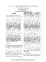
At the beginning of each round for feature se-
lection, a uniform prior distribution is always
assumed for the new CME model. A more pre-
cise description of the PFS algorithm is given in
Table 1, and it is also graphically illustrated in
Figure 1.
Given:

Feature space
F
(0)
=
{f
1
(0)
, f
2
(0)
, …, f
N
(0)
},
step_num =
m, select_factor = s
1. Split the feature space into
N
1
parts

{
F
1
(1)
,
F
2
(1)

, …,
F
N
1
(1)
} = split(
F
(0)
)
2. for
k
=1 to m-1
do
//2.1 Feature selection

for
each feature space
F
i
(k)

do


FS
i
(k)

= SGC(
F

i
(k)
, s)
//
2.2

Combine selected features

{
F
1
(k+1)
, …,
F
N
k+1
(k+1)
}

=
merge(
FS
1
(k)
, …,
FS
N
k
(k)
)

3. Final feature selection & optimization
F
(m)
= merge(
FS
1
(m-1)
, …,
FS
N
m-1
(m-1)
)
FS
(m)

= SGC(
F
(m)
, s)
M
final
= Opt(
FS
(m)
)

Table 1. The PFS algorithm.

M
)2(
1
F
)1(
1
FS
)1(
1
i
FS
M
M
)1(
2
i
FS
M
)1(
1
N
FS
L
select
Step 1
Step m
)1(
1
F
)1(

1
i
F
M
M
)1(
2
i
F
M
)1(
1
N
F
)2(
1
FS
)2(
2
N
FS
)(m
F
M
merge
Step 2
)0(
F
Split
select merge

select
)2(
2
N
F
M
final

)(m
FS
optimize
Figure 1. Graphic illustration of PFS algorithm.

In Table 1, SGC() invokes the SGC algorithm,
and Opt() optimizes feature weights. The func-
tions split() and merge() are used to split and
merge the feature space respectively.
Two variations of the split() function are in-
vestigated in the paper and they are described
below:
1. random-split: randomly split a feature
space into n- disjoint subspaces, and select
an equal amount of features for each fea-
ture subspace.
2. dimension-based-split: split a feature
space into disjoint subspaces based on fea-
563
ture dimensions/variables, and select the
number of features for each feature sub-
space with a certain distribution.

We use a simple method for merge() in the
experiments reported here, i.e., adding together
the features from a set of selected feature sub-
spaces.
One may image other variations of the split()
function, such as allowing overlapping sub-
spaces. Other alternatives for merge() are also
possible, such as randomly grouping the selected
feature subspaces in the dimension-based split.
Due to the limitation of the space, they are not
discussed here.
This approach can in principle be applied to
other machine learning algorithms as well.
4 Experiments with PFS for Edit Re-
gion Identification
In this section, we will demonstrate the benefits
of the PFS algorithm for identifying edit regions.
The main reason that we use this task is that the
edit region detection task uses features from sev-
eral levels, including prosodic, lexical, and syn-
tactic ones. It presents a big challenge to find a
set of good features from a huge feature space.
First we will present the additional features
that the PFS algorithm allows us to include.
Then, we will briefly introduce the variant of the
Switchboard corpus used in the experiments. Fi-
nally, we will compare results from two variants
of the PFS algorithm.
4.1 Edit Region Identification Task
In spoken utterances, disfluencies, such as self-

editing, pauses and repairs, are common phe-
nomena. Charniak and Johnson (2001) and Kahn
et al. (2005) have shown that improved edit re-
gion identification leads to better parsing accu-
racy – they observe a relative reduction in pars-
ing f-score error of 14% (2% absolute) between
automatic and oracle edit removal.
The focus of our work is to show that our new
PFS algorithm enables the exploration of much
larger feature spaces for edit identification – in-
cluding prosodic features, their confidence
scores, and various feature combinations – and
consequently, it further improves edit region
identification. Memory limitation prevents us
from including all of these features in experi-
ments using the boosting method described in
Johnson and Charniak (2004) and Zhang and
Weng (2005). We couldn’t use the new features
with the SGC algorithm either for the same rea-
son.
The features used here are grouped according
to variables, which define feature sub-spaces as
in Charniak and Johnson (2001) and Zhang and
Weng (2005). In this work, we use a total of 62
variables, which include 16
1
variables from
Charniak and Johnson (2001) and Johnson and
Charniak (2004), an additional 29 variables from
Zhang and Weng (2005), 11 hierarchical POS tag

variables, and 8 prosody variables (labels and
their confidence scores). Furthermore, we ex-
plore 377 combinations of these 62 variables,
which include 40 combinations from Zhang and
Weng (2005). The complete list of the variables
is given in Table 2, and the combinations used in
the experiments are given in Table 3. One addi-
tional note is that some features are obtained af-
ter the rough copy procedure is performed, where
we used the same procedure as the one by Zhang
and Weng (2005). For a fair comparison with the
work by Kahn et al. (2005), word fragment in-
formation is retained.
4.2 The Re-segmented Switchboard Data
In order to include prosodic features and be able
to compare with the state-oft-art, we use the
University of Washington re-segmented
Switchboard corpus, described in Kahn et al.
(2005). In this corpus, the Switchboard sentences
were segmented into V5-style sentence-like units
(SUs) (LDC, 2004). The resulting sentences fit
more closely with the boundaries that can be de-
tected through automatic procedures (e.g., Liu et
al., 2005). Because the edit region identification
results on the original Switchboard are not di-
rectly comparable with the results on the newly
segmented data, the state-of-art results reported
by Charniak and Johnson (2001) and Johnson
and Charniak (2004) are repeated on this new
corpus by Kahn et al. (2005).

The re-segmented UW Switchboard corpus is
labeled with a simplified subset of the ToBI pro-
sodic system (Ostendorf et al., 2001). The three
simplified labels in the subset are p, 1 and 4,
where p refers to a general class of disfluent
boundaries (e.g., word fragments, abruptly short-
ened words, and hesitation); 4 refers to break
level 4, which describes a boundary that has a
boundary tone and phrase-final lengthening;

1
Among the original 18 variables, two variables, P
f
and T
f

are not used in our experiments, because they are mostly
covered by the other variables. Partial word flags only con-
tribute to 3 features in the final selected feature list.
564
Categories Variable Name Short Description
Orthographic
Words
W
-5
, … , W
+5

Words at the current position and the left and right 5
positions.

Partial Word Flags P
-3
, …, P
+3

Partial word flags at the current position and the left
and right 3 positions
Words
Distance D
INTJ,
D
W,
D
Bigram
, D
Trigram
Distance features
POS Tags T
-5
, …, T
+5

POS tags at the current position and the left and
right 5 positions.
Tags
Hierarchical
POS Tags (HTag)
HT
-5
, …, HT

+5

Hierarchical POS tags at the current position and the
left and right 5 positions.
HTag Rough Copy N
m
, N
n
, N
i
, N
l
, N
r
, T
i
Hierarchical POS rough copy features.
Rough Copy
Word Rough Copy WN
m
, WN
i
, WN
l
, WN
r
Word rough copy features.
Prosody Labels PL
0
, …, PL

3

Prosody label with largest post possibility at the
current position and the right 3 positions.
Prosody
Prosody Scores PC
0
, …, PC
3

Prosody confidence at the current position and the
right 3 positions.
Table 2. A complete list of variables used in the experiments.

Categories Short Description
Number of
Combinations
Tags HTagComb Combinations among Hierarchical POS Tags 55
Words OrthWordComb Combinations among Orthographic Words 55
Tags
WTComb
WTTComb
Combinations of Orthographic Words and POS
Tags; Combination among POS Tags
176
Rough Copy RCComb
Combinations of HTag Rough Copy and Word
Rough Copy
55
Prosody PComb Combinations among Prosody, and with Words 36

Table 3. All the variable combinations used in the experiments.

and 1 is used to include the break index levels
BL 0, 1, 2, and 3. Since the majority of the cor-
pus is labeled via automatic methods, the f-
scores for the prosodic labels are not high. In
particular, 4 and p have f-scores of about 70%
and 60% respectively (Wong et al., 2005). There-
fore, in our experiments, we also take prosody
confidence scores into consideration.
Besides the symbolic prosody labels, the cor-
pus preserves the majority of the previously an-
notated syntactic information as well as edit re-
gion labels.
In following experiments, to make the results
comparable, the same data subsets described in
Kahn et al. (2005) are used for training, develop-
ing and testing.
4.3 Experiments
The best result on the UW Switchboard for edit
region identification uses a TAG-based approach
(Kahn et al., 2005). On the original Switchboard
corpus, Zhang and Weng (2005) reported nearly
20% better results using the boosting method
with a much larger feature space
2
. To allow
comparison with the best past results, we create a
new CME baseline with the same set of features
as that used in Zhang and Weng (2005).

We design a number of experiments to test the
following hypotheses:
1. PFS can include a huge number of new
features, which leads to an overall per-
formance improvement.
2. Richer context, represented by the combi-
nations of different variables, has a posi-
tive impact on performance.
3. When the same feature space is used, PFS
performs equally well as the original SGC
algorithm.
The new models from the PFS algorithm are
trained on the training data and tuned on the de-
velopment data. The results of our experiments
on the test data are summarized in Table 4. The
first three lines show that the TAG-based ap-
proach is outperformed by the new CME base-
line (line 3) using all the features in Zhang and
Weng (2005). However, the improvement from

2
PFS is not applied to the boosting algorithm at this time
because it would require significant changes to the available
algorithm.
565
Results on test data
Feature Space Codes
number of
features
Precision Recall F-Value

TAG-based result on UW-SWBD reported in Kahn et al. (2005)


78.20
CME with all the variables from Zhang and Weng (2005) 2412382 89.42 71.22 79.29
CME with all the variables from Zhang and Weng (2005) + post 2412382 87.15 73.78
79.91
+HTag +HTagComb +WTComb +RCComb 17116957 90.44 72.53 80.50
+HTag +HTagComb +WTComb +RCComb +PL
0
… PL
3
17116981 88.69 74.01 80.69
+HTag +HTagComb +WTComb +RCComb +PComb: without cut 20445375 89.43 73.78 80.86
+HTag +HTagComb +WTComb +RCComb +PComb: cut2 19294583 88.95 74.66
81.18
+HTag +HTagComb +WTComb +RCComb +PComb: cut2 +Gau 19294583 90.37 74.40 81.61
+HTag +HTagComb +WTComb +RCComb +PComb: cut2 +post 19294583 86.88 77.29 81.80
+HTag +HTagComb +WTComb +RCComb +PComb: cut2 +Gau
+post
19294583 87.79 77.02
82.05
Table 4. Summary of experimental results with PFS.

CME is significantly smaller than the reported
results using the boosting method. In other
words, using CME instead of boosting incurs a
performance hit.
The next four lines in Table 4 show that addi-
tional combinations of the feature variables used

in Zhang and Weng (2005) give an absolute im-
provement of more than 1%. This improvement
is realized through increasing the search space to
more than 20 million features, 8 times the maxi-
mum size that the original boosting and CME
algorithms are able to handle.
Table 4 shows that prosody labels alone make
no difference in performance. Instead, for each
position in the sentence, we compute the entropy
of the distribution of the labels’ confidence
scores. We normalize the entropy to the range [0,
1], according to the formula below:

() ( )
UniformHpHscore −= 1 (4)
Including this feature does result in a good
improvement. In the table, cut2 means that we
equally divide the feature scores into 10 buckets
and any number below 0.2 is ignored. The total
contribution from the combined feature variables
leads to a 1.9% absolute improvement. This con-
firms the first two hypotheses.
When Gaussian smoothing (Chen and
Rosenfeld, 1999), labeled as +Gau, and post-
processing (Zhang and Weng, 2005), labeled as
+post, are added, we observe 17.66% relative
improvement (or 3.85% absolute) over the previ-
ous best f-score of 78.2 from Kahn et al. (2005).
To test hypothesis 3, we are constrained to the
feature spaces that both PFS and SGC algorithms

can process. Therefore, we take all the variables
from Zhang and Weng (2005) as the feature
space for the experiments. The results are listed
in Table 5. We observed no f-score degradation
with PFS. Surprisingly, the total amount of time
PFS spends on selecting its best features is
smaller than the time SGC uses in selecting its
best features. This confirms our hypothesis 3.

Results on test data
Split / Non-split
Precision Recall F-Value
non-split 89.42 71.22 79.29
split by 4 parts 89.67 71.68 79.67
split by 10 parts 89.65 71.29 79.42
Table 5. Comparison between PFS and SGC with
all the variables from Zhang and Weng (2005).

The last set of experiments for edit identifica-
tion is designed to find out what split strategies
PFS algorithm should adopt in order to obtain
good results. Two different split strategies are
tested here. In all the experiments reported so far,
we use 10 random splits, i.e., all the features are
randomly assigned to 10 subsets of equal size.
We may also envision a split strategy that divides
the features based on feature variables (or dimen-
sions), such as word-based, tag-based, etc. The
four dimensions used in the experiments are
listed as the top categories in Tables 2 and 3, and

the results are given in Table 6.

Results on test data Split
Criteria
Allocation
Criteria
Precision Recall F-Value
Random Uniform 88.95 74.66 81.18
Dimension Uniform 89.78 73.42 80.78
Dimension Prior 89.78 74.01 81.14
Table 6. Comparison of split strategies using feature space
+HTag+HTagComb+WTComb+RCComb+PComb: cut2

In Table 6, the first two columns show criteria
for splitting feature spaces and the number of
features to be allocated for each group. Random
and Dimension mean random-split and dimen-
sion-based-split, respectively. When the criterion
566
is Random, the features are allocated to different
groups randomly, and each group gets the same
number of features. In the case of dimension-
based split, we determine the number of features
allocated for each dimension in two ways. When
the split is Uniform, the same number of features
is allocated for each dimension. When the split is
Prior, the number of features to be allocated in
each dimension is determined in proportion to
the importance of each dimension. To determine
the importance, we use the distribution of the

selected features from each dimension in the
model “+ HTag + HTagComb + WTComb +
RCComb + PComb: cut2”, namely: Word-based
15%, Tag-based 70%, RoughCopy-based 7.5%
and Prosody-based 7.5%
3
. From the results, we
can see no significant difference between the
random-split and the dimension-based-split.
To see whether the improvements are trans-
lated into parsing results, we have conducted one
more set of experiments on the UW Switchboard
corpus. We apply the latest version of Charniak’s
parser (2005-08-16) and the same procedure as
Charniak and Johnson (2001) and Kahn et al.
(2005) to the output from our best edit detector
in this paper. To make it more comparable with
the results in Kahn et al. (2005), we repeat the
same experiment with the gold edits, using the
latest parser. Both results are listed in Table 7.
The difference between our best detector and the
gold edits in parsing (1.51%) is smaller than the
difference between the TAG-based detector and
the gold edits (1.9%). In other words, if we use
the gold edits as the upper bound, we see a rela-
tive error reduction of 20.5%.

Parsing F-score
Methods
Edit

F-score
Reported
in Kahn et
al. (2005)
Latest
Charniak
Parser
Diff.
with
Oracle
Oracle 100 86.9 87.92
Kahn et
al. (2005)
78.2 85.0
1.90
PFS best
results
82.05 86.41
1.51
Table 7. Parsing F-score various different edit
region identification results.

3
It is a bit of cheating to use the distribution from the se-
lected model. However, even with this distribution, we do
not see any improvement over the version with random-
split.
5 Conclusion
This paper presents our progressive feature selec-
tion algorithm that greatly extends the feature

space for conditional maximum entropy model-
ing. The new algorithm is able to select features
from feature space in the order of tens of mil-
lions in practice, i.e., 8 times the maximal size
previous algorithms are able to process, and
unlimited space size in theory. Experiments on
edit region identification task have shown that
the increased feature space leads to 17.66% rela-
tive improvement (or 3.85% absolute) over the
best result reported by Kahn et al. (2005), and
10.65% relative improvement (or 2.14% abso-
lute) over the new baseline SGC algorithm with
all the variables from Zhang and Weng (2005).
We also show that symbolic prosody labels to-
gether with confidence scores are useful in edit
region identification task.
In addition, the improvements in the edit iden-
tification lead to a relative 20% error reduction in
parsing disfluent sentences when gold edits are
used as the upper bound.
Acknowledgement
This work is partly sponsored by a NIST ATP
funding. The authors would like to express their
many thanks to Mari Ostendorf and Jeremy Kahn
for providing us with the re-segmented UW
Switchboard Treebank and the corresponding
prosodic labels. Our thanks also go to Jeff Rus-
sell for his careful proof reading, and the anony-
mous reviewers for their useful comments. All
the remaining errors are ours.

References
Adam L. Berger, Stephen A. Della Pietra, and Vin-
cent J. Della Pietra. 1996. A Maximum Entropy
Approach to Natural Language Processing. Com-
putational Linguistics, 22 (1): 39-71.
Eugene Charniak and Mark Johnson. 2001. Edit De-
tection and Parsing for Transcribed Speech. In
Proceedings of the 2
nd
Meeting of the North Ameri-
can Chapter of the Association for Computational
Linguistics, 118-126, Pittsburgh, PA, USA.
Eugene Charniak and Mark Johnson. 2005. Coarse-to-
fine n-best Parsing and MaxEnt Discriminative
Reranking. In Proceedings of the 43
rd
Annual
Meeting of Association for Computational Linguis-
tics, 173-180, Ann Arbor, MI, USA.
Stanley Chen and Ronald Rosenfeld. 1999. A Gaus-
sian Prior for Smoothing Maximum Entropy Mod-
567
els. Technical Report CMUCS-99-108, Carnegie
Mellon University.
John N. Darroch and D. Ratcliff. 1972. Generalized
Iterative Scaling for Log-Linear Models. In Annals
of Mathematical Statistics, 43(5): 1470-1480.
Stephen A. Della Pietra, Vincent J. Della Pietra, and
John Lafferty. 1997. Inducing Features of Random
Fields. In IEEE Transactions on Pattern Analysis

and Machine Intelligence, 19(4): 380-393.
Joshua Goodman. 2002. Sequential Conditional Gen-
eralized Iterative Scaling. In Proceedings of the
40
th
Annual Meeting of Association for Computa-
tional Linguistics, 9-16, Philadelphia, PA, USA.
Mark Johnson, and Eugene Charniak. 2004. A TAG-
based noisy-channel model of speech repairs. In
Proceedings of the 42
nd
Annual Meeting of the As-
sociation for Computational Linguistics, 33-39,
Barcelona, Spain.
Jeremy G. Kahn, Matthew Lease, Eugene Charniak,
Mark Johnson, and Mari Ostendorf. 2005. Effec-
tive Use of Prosody in Parsing Conversational
Speech. In Proceedings of the 2005 Conference on
Empirical Methods in Natural Language Process-
ing, 233-240, Vancouver, Canada.
Rob Koeling. 2000. Chunking with Maximum En-
tropy Models. In Proceedings of the CoNLL-2000
and LLL-2000, 139-141, Lisbon, Portugal.
LDC. 2004. Simple MetaData Annotation Specifica-
tion. Technical Report of Linguistic Data Consor-
tium. (
Yang Liu, Elizabeth Shriberg, Andreas Stolcke, Bar-
bara Peskin, Jeremy Ang, Dustin Hillard, Mari Os-
tendorf, Marcus Tomalin, Phil Woodland and Mary
Harper. 2005. Structural Metadata Research in the

EARS Program. In Proceedings of the 30
th

ICASSP, volume V, 957-960, Philadelphia, PA,
USA.
Robert Malouf. 2002. A Comparison of Algorithms
for Maximum Entropy Parameter Estimation. In
Proceedings of the 6
th
Conference on Natural Lan-
guage Learning (CoNLL-2002), 49-55, Taibei,
Taiwan.
Mari Ostendorf, Izhak Shafran, Stefanie Shattuck-
Hufnagel, Leslie Charmichael, and William Byrne.
2001. A Prosodically Labeled Database of Sponta-
neous Speech. In Proceedings of the ISCA Work-
shop of Prosody in Speech Recognition and Under-
standing, 119-121, Red Bank, NJ, USA.
Adwait Ratnaparkhi, Jeff Reynar and Salim Roukos.
1994. A Maximum Entropy Model for Preposi-
tional Phrase Attachment. In Proceedings of the
ARPA Workshop on Human Language Technology,
250-255, Plainsboro, NJ, USA.
Jeffrey C. Reynar and Adwait Ratnaparkhi. 1997. A
Maximum Entropy Approach to Identifying Sen-
tence Boundaries. In Proceedings of the 5
th
Con-
ference on Applied Natural Language Processing,
16-19, Washington D.C., USA.

Stefan Riezler and Alexander Vasserman. 2004. In-
cremental Feature Selection and L1 Regularization
for Relaxed Maximum-entropy Modeling. In Pro-
ceedings of the 2004 Conference on Empirical
Methods in Natural Language Processing, 174-
181, Barcelona, Spain.
Robert E. Schapire and Yoram Singer, 1999. Im-
proved Boosting Algorithms Using Confidence-
rated Predictions. Machine Learning, 37(3): 297-
336.
Elizabeth Shriberg. 1994. Preliminaries to a Theory
of Speech Disfluencies. Ph.D. Thesis, University of
California, Berkeley.
Vladimir Vapnik. 1995. The Nature of Statistical
Learning Theory. Springer, New York, NY, USA.
Darby Wong, Mari Ostendorf, Jeremy G. Kahn. 2005.
Using Weakly Supervised Learning to Improve
Prosody Labeling. Technical Report UWEETR-
2005-0003, University of Washington.
Qi Zhang and Fuliang Weng. 2005. Exploring Fea-
tures for Identifying Edited Regions in Disfluent
Sentences. In Proc. of the 9
th
International Work-
shop on Parsing Technologies, 179-185, Vancou-
ver, Canada.
Yaqian Zhou, Fuliang Weng, Lide Wu, and Hauke
Schmidt. 2003. A Fast Algorithm for Feature Se-
lection in Conditional Maximum Entropy Model-
ing. In Proceedings of the 2003 Conference on

Empirical Methods in Natural Language Process-
ing, 153-159, Sapporo, Japan.
568