MauveDB: Supporting Model-based User Views in Database Systems pptx

MauveDB: Supporting Model-based User Views in
Database Systems
Amol Deshpande Samuel Madden

University of Maryland MIT
ABSTRACT
Real-world data — especially when generated by distributed
measurement infrastructures such as sensor networks — tends
to be incomplete, imprecise, and erroneous, making it im-
possible to pres ent it to users or feed it directly into applica-
tions. The traditional approach to dealing with this problem
is to first process the data using statistical or probabilistic
models that can provide more robust interpretations of the
data. Current database systems, however, do not provide
adequate support for applying models to such data, espe-
cially when those models need to be frequently updated as
new data arrives in the system. Hence, most scientists and
engineers who depend on models for managing their data do
not use database systems for archival or querying at all; at
best, databases serve as a persistent raw data store.
In this paper we define a new abstraction called model-
based views and present the architecture of MauveDB, the
system we are building to support such views. Just as tra-
ditional database views provide logical data independence,
mo del-based views provide independence from the details
of the underlying data generating mechanism and hide the
irregularities of the data by using models to present a con-
sistent view to the users. MauveDB supports a declarative
language for defining model-based views, allows declarative
querying over such views using SQL, and supports several
different materialization strategies and techniques to effi-

ciently maintain them in the face of frequent updates. We
have implemented a prototype system that currently sup-
ports views based on regression and interpolation, using
the Apache Derby open source DBMS, and we present re-
sults that show the utility and performance benefits that can
be obtained by supporting several different types of model-
based views in a database system.
1. INTRODUCTION
mod◦el |’m¨adl|
noun
a simplified description, esp. a mathematical one,
of a system or process, to assist in calculations
and predictions: a statistical model for predicting
the survival rates of endangered species.[30]
Permission to make digital or hard copies of all or part of this work for
personal or classroom use is granted without fee provided that copies are
not made or distributed for profit or commercial advantage and that copies
bear this notice and the full citation on the first page. To copy otherwise, to
republish, to post on servers or to redistribute to lists, requires prior specific
permission and/or a fee.
SIGMOD 2006, June 27–29, 2006, Chicago, Illinois, USA
Copyright 2006 ACM 1-59593-256-9/06/0006 5.00.
Given the benefits that a database system provides for
structuring data and preserving its durability and integrity,
one might expect to find scientists and engineers making ex-
tensive use of database systems to manage their data. Un-
fortunately, domains such as biology, chemistry, mechanical
engineering (and a variety of others ) typically use databases
in only the most rudimentary of ways, running few or no
queries and storing only raw observations as they are cap-

tured from sensors or other field instruments. This is be-
cause the real-world data acquired using such measurement
infrastructures is typically incomplete, imprecise, and erro-
neous, and hence rarely usable as it is. The raw data needs
to be synthesized (filtered) using models, simplified mathe-
matical descriptions of the underlying systems or processes,
before it can be used. Physical scientists, for instance, use
mo dels all of the time: to predict weather, to approximate
temp erature and rainfall distributions, or to estimate the
flow of traffic on a road segment near a traffic accident. In
recent years, the need for such modeling has moved out of
the realm of scientific data management alone, mainly as a
result of an increasing number of deployments of large-scale
measurement infrastructures such as sensor networks that
tend to produce similar noisy data.
Unfortunately there is a lack of effective data management
to ols that can help users in managing such data and in ap-
plying models, forcing them to use external tools for this
purpose. Scientists, for instance, typically import the raw
data into an analysis package such as Matlab, where they
apply various models to the data. Once the data has been
filtered, they typically process it further using customized
programs that are often quite similar to database queries
(e.g., that find peaks in the cleaned data, extract particu-
lar subsets, or compute aggregates over different regions).
It is impractical for them to use databases for this later
pro ces sing, because data has already been extracted from
the database and re-inserting is slow and awkward. This
seriously limits the utility of databases for many mo de l-
based applications and requires scientists and other users to

waste huge amounts of time w riting custom data process-
ing code on the output of their models. Some traditional
database systems do support querying of statistical models
(e.g., DB2’s Intelligent Miner [20] adds support for models
defined in the PMML language to DB2), but they tend to
abstract models simply as user defined functions that can
be applied to raw data tables. Unfortunately, this level of
integration of models and databases is insufficient for many
applications as there is no support for efficiently maintain-
ing models or for updating their parameters when new data
1
This work was supported by NSF Grants CNS-0509220, IIS-
0546136, CNS-0509261, and IIS-044814.
is inserted into the system (in some cases, many thousands
of new readings may be inserted per day).
1.1 Example: Wireless Sensor Networks
To illustrate an application of modeling and the pitfalls
of scientific data management, we consider a wireless sensor
networking application. Wireless sensor networks consist of
tiny, battery-powered, multi-function s ens or nodes that can
communicate over short distances using radios. Such net-
works have the potential to enable a wide range of applica-
tions in environmental monitoring, health, military and se-
curity (see [1] for a survey of applications). There have been
several large-scale deployments of such sensor networks that
have collected highly useful data in many domains (e.g., [29,
6, 5]). Many of the deployments demonstrate the limited-use
of databases described above: a DBMS is used to capture
and store the raw data, but all of the data modeling and
analysis is done outside of the database system.

This is because wireless sensor networks rarely produce
“clean” and directly usable data. Sensor and communication
link failures typically result in significant amounts of incom-
plete data. Sensors also tend to be error-prone, sometimes
producing erroneous data without any other indication of a
failure. In addition, it is rarely possible to instrument the
physical world exactly the way the application or the user
desires. As an example, an HVAC (Heating, Ventilation, and
Air Conditioning) system that uses temperature sensors to
measure temperatures in various parts of the building, would
want to know, at all times, the temperatures in all rooms in
the building. However, the data collected from the sensor
network may not match this precisely; at some times, we
may not have data from certain rooms, and certain (large)
rooms may have multiple monitoring sensors. In addition,
the sensors may not be able to measure the temperatures
at precisely the times the HVAC system demands. Finally,
sensors may be added or removed at will by the building ad-
ministrator for various reasons such as a desire for increased
accuracy or to handle failures.
Many of these problems can be resolved by putting an
additional layer of software between the raw sensor data
and the application that uses a model to filter the raw data
and to present the application with a consistent “view” of
the system. A variety of models can be used for this pur-
pose. For example, regression and interpolation models can
be used to predict missing or future data, and also to handle
spatial or temporal non-uniformity. Similarly dynamic prob-
abilistic models and linear dynamical systems (e.g., Kalman
Filters) can be used for eliminating white noise, for error

detection, and also for prediction.
Trying to use existing tools to implement this software
layer, however, is problematic. For instance, we could try
to use a modeling tool (like Intelligent Miner’s IM Modeling
to ol) to learn a regressive model that predicts temperature
at any location from a training set of (X,Y,temperature) tu-
ples. We could then use this model as a UDF in a DBMS
to predict temperature from input (X,Y) values. Unfortu-
nately, if a new set of sensor readings that we would like to
have affect the predictions of the model is inserted into the
database, we would have to explicitly re-run the modeling
to ol and reload the model into the system, which would be
both slow and awkward. Using Matlab or some other dedi-
cated modeling tool presents even more serious problems as
it provides no support for native data storage, and querying.
1.2 New Abstraction: Model-based Views
In this paper we propose to rectify this situation via a new
abstraction called model-based views which we have imple-
mented in a traditional relational database system. Model-
based views abstract away the details of the underlying mea-
surement infrastructure and hide the irregularities of the
data by using models to present a consistent view — over
space and time — to the users or the applications that are
using the data. Our system, called MauveDB(Model-based
User Views)
2
, extends an existing relational DBMS (Apache
Derby), and not only allows users to specify and create
mo del-based views, but also provides transparent s upport
for querying such views and keeping them up-to-date as the

underlying raw data table is updated. The salient features
of MauveDB are:
• MauveDB’s model-based views act as an “independence”
layer between raw sensor data and the user/application
view of the state of the world. This helps insulate the
user or the application from the messy details of the
underlying measurement infrastructure.
• MauveDB provides language constructs for declara-
tively specifying views based on a variety of commonly
used models. We describe several such models that we
have implemented in our prototype system, as well as
our approach for defining arbitrary model-based views.
• MauveDB supports declarative queries over model-based
views using unmodified SQL.
• MauveDB does not simply apply models to static data;
rather, as the underlying raw data is modified, MauveDB
keeps the outputs of the model consistent with these
changes. We describe a number of techniques we have
developed to do this maintenance efficiently.
Finally, we emphasize that the goal of this paper is not
to advocate particular models for particular types of data
or domains, but to show that it possible to build a database
system that seamlessly and efficiently integrates the use and
updating of models over time. Though we provide a num-
ber of examples of situations in which modeling is useful
and show how models can improve data quality significantly,
many real world domains would use the models we discuss
here in concert with other models or in somewhat more so-
phisticated ways than we present.
1.3 Outline

We begin by elaborating on our proposed abs traction of
mo del-based views, and discuss how these views are exposed
to the database users (Section 2). We then present the ar-
chitecture of MauveDB, the DBMS that we are building to
support model-based views, and discuss view creation, view
maintenance and query evaluation issues (Section 3). In
Section 4, we describe some more specific details of our pro-
totype implementation of MauveDB in the Apache Derby
DBMS, followed by an experimental study of our implemen-
tation in Section 5.
2. MODEL-BASED VIEWS
Relational database systems are fundamentally based on
the notion of data independence, where low-level details are
2
In a famous Dilbert cartoon, the pointy-haired boss asks Dilbert
to build a mauve-colored SQL database because “mauve has the
most RAM”.
t=0
t=0
t=1
t=1
t=2
t=2
User View (uniform at all times)
Actual Observations Made at Various Times
time x y temp
0 1 1 20
0 15 10 18
1 10 8 15
time x y temp

0 10 10 19.5
1 10 10 16
0 10 20 20.5
ModelView
raw-temp-readings
10 200
10
10 200
10
10 200
10
Model projects from raw readings onto grid
Figure 1: Model-based view ModelView defined over the raw sensor data table raw-temp-readings: The user
always sees only the (model-predicted) temperatures at the grid points, irrespective of where the actual
measurements were made.
hidden underneath layers of abstraction. Database views
provide one such important layer, where the logical view
provided to the users may be different from the physical
representation of the data on disk. In MauveDB, we gen-
eralize this notion by allowing database views to be defined
using statistical models instead of just SQL queries; we call
such views model-based views.
To elaborate on the abstraction of model-based views, we
use an example of a wireless sensor network deployment that
is monitoring the temperatures in two-dimensional space.
We assume that the database contains a raw data table with
the schema: raw-temp-readings(time, x, y, temp, sensorid),
into which all readings received from the sensor network are
inserted (in real-time). The sensorid attribute records the
unique id that has been assigned to the sensor making the

measurement.
2.1 Models as Tables
We begin with a discussion of exactly what the contents
of a model-based view are (in other words, the result of the
select * query on the view).
Assuming that the statistical model we are using allows
us to predict the temperature at any coordinate in this 2D
space (as do the models we discuss below), the natural way
to present this model to a user is as a uniform grid-based
approximation (Figure 1). This representation provides an
approximation of the attribute space as a relational table
with a finite number of rows. The granularity of the grid
is specified in the view definition statement. At each time
instance, we can use the model (after possibly learning the
parameters from the observed raw data) to predict the val-
ues at each grid point using the known values in the raw
data. Figure 1 depicts the raw data at different times being
projected onto a uniform two dimensional grid at each time
step. As we can see, though the schema of the view (Mod-
elView) is identical to the schema of the raw data in (raw-
temp-readings), the user always sees temperatures at exactly
the grid-points, irrespective of the locations and times of the
actual observations in the raw data table
3
. Presenting the
user with such a view has several significant advantages:
3
Some models may extend the schema of the prediction column
by providing a confidence bound or error estimate on each pre-
diction; n eith er the regression o r interpolation techniques used as

• The underlying sensor network can be transparently
changed (e.g., new sensor nodes can be added, or
failed nodes can be removed) without affecting the ap-
plications written on top of it. Similarly, the system
masks missing data by preserving this regular view.
• Any spatial or temporal biases in the measure-
ments are naturally removed. For example, an av-
erage query over this view will return a spatially un-
biased estimate. Running such a query over the raw
sensor data will typically not provide an unbiased es-
timate.
It is important to note that this is only a conceptual view
of the data presented to the user, and it is usually pos-
sible to avoid completely materializing this whole table in
MauveDB; instead, for most types of views, an intermedi-
ate representation can be maintained that allows us to ef-
ficiently compute the value at any grid point on demand
(Section 3.3.2).
2.2 Examples
To illustrate how gridded model-based views work, we
present two examples based on the standard mo deling tools
of regression and interpolation.
2.2.1 Example 1: Regression-based Views
Regression techniques are routinely and very successfully
used in many application domains to model the values of a
continuous dependent variable as a function of the values of
a set of independent or predictor variables. These models are
thus a natural fit in many environmental monitoring appli-
cations that use sensor networks to monitor physical prop-
erties such as temperature, humidity, light etc. Guestrin et

al [17], for example, demonstrate how kernel linear regres-
sion can be successfully used to model the temperature in an
indo or setting in a real sensor network deployment.
In our running example above, we can use regression to
mo del the temp as a function of the geographical location
(x, y) as:
temp(x, y) = Σ
k
i=1
w
i
h
i
(x, y)
where h
i
(x, y) are called the basis functions (that are typi-
examples in this paper naturally provide such error bounds.
0 5 10 15
0
20
40
60
Cubic Fit
y=a + bx + cx
2
+ dx
3
0 5 10 15
0

20
40
60
Quadratic Fit
y=a + bx + cx
2
0 5 10 15
0
20
40
60
Linear Fit
y=a + bx
Figure 2: Example of regression with three different
sets of basis functions.
cally pre-defined), and w
i
are called the weights. An exam-
ple set of basis functions might be h
1
(x, y) = 1, h
2
(x, y) =
x, h
3
(x, y) = x
2
, h
4
(x, y) = y, h

5
(x, y) = y
2
, in which case,
temp is computed as:
temp(x, y) = w
1
+ w
2
x + w
3
x
2
+ w
4
y + w
4
y
2
The goal of regression modeling is to find the optimal weights,
w
∗
i
, that minimize some error metric given a set of obser-
vations, i.e., temperature measurements at a subset of the
lo cations, temp(x
i
, y
i
) = temp

i
, i = 1, . . . , m. The most
commonly used error metric is the root mean squared error
(RMS), e.g.:
r
1
m
Σ
m
j=1
(temp
j
− Σ
k
i=1
w
i
h
i
(x
j
, y
j
))
2
Once the optimal weights have been computed by mini-
mizing this expression, we can then use the regression func-
tion to estimate the temperature at any location in the 2-
dimensional space under consideration.
Figure 2 illustrates the results of linear regression with

three different sets of basis functions (shown on each of the
three sub-graphs.) In general, adding additional terms to
a basis function improves the quality of fit but also tends
to lead to over-fitting where new observations are not well
predicted by the existing model because the model is com-
pletely specialized to the existing data.
To solve this optimization problem using linear regression,
we need to define two matrices:
H =
0
B
@
h
1
(x
1
, y
1
) . . . h
k
(x
1
, y
1
)
.
.
.
.
.

.
.
.
.
h
1
(x
m
, y
m
) . . . h
k
(x
m
, y
m
)
1
C
A
, f =
0
B
@
temp
1
.
.
.
temp

m
1
C
A
(1)
It is well known [14] that the optimal weights w
∗
= (w
∗
1
, . . . , w
∗
k
)
that minimize the RMS error can then be computed by solv-
ing the following system of equations:
H
T
H w
∗
= H
T
f
The simplest implementation of regression-based views in
MauveDB simply uses Gaussian Elimination [14] to do this.
User Representation: To use a regression-based view,
the user writes a view definition that tells MauveDB to fit a
particular set of raw data using a particular set of regression
basis functions (the view definition language is discussed in
more detail in Section 3.1). Since the regression function

fits the generic model discussed in Section 2.1 above, we can
use the uniform, grid-based approximation discussed there
to present the outputs of the regression function to the user.
2.2.2 Example 2: Interpolation-based Views
We describe a second ty pe of view in this se ction, the in-
terpolation view. In an interpolation view an interpolation
0 5 10 15
0
20
40
60
Nearest Neighbor Interpolation
0 5 10 15
0
20
40
60
Linear Interpolation
0 5 10 15
0
20
40
60
Spline Interpolation
Figure 3: Example of interpolation with three dif-
ferent interpolation functions.
time
temperature
Query: At what time was the temperature equal to temp'?
temp'

No Interpolation
time
Linear Interpolation
Answer = { }
T'
Answer = { T' }
Figure 4: Example showing the use of interpola-
tion to identify the time T

when the temperat ure
is equal to t

.
function is used to estimate the missing values from known
values that bracket the missing value. The process is sim-
ilar to table lookup: given a table T of tuples of the form
(T, V ), and a set of T

values with unknown V

values, we
can estimate the v

∈ V

value that corresponds to a par-
ticular t

∈ T


by looking up two pairs (t
1
, v
1
) and (t
2
, v
2
)
in T such that t
1
≤ t

≤ t
2
. We then use the interpolation
function to compute the value v

from v
1
and v
2
.
Interpolation presents a natural way to fill in missing val-
ues in the wireless sensor network application. In sens or
network database systems like Cougar [38] and TinyDB [28],
which report sensor readings on a periodic schedule, typi-
cally only a fraction of the nodes report during each time
interval, since many messages are lost in-transit in the net-
work. If the user of one of these sy stems wants to compute

an aggregate over the data, missing readings can lead to
very unpredictable behavior – an average or a maximum,
for example, may appear to fluctuate dramatically from one
time period to the next. By interpolating missing values,
aggregates are much more stable (and closer to the true an-
swer). For example, suppose we have heard sensor readings
from a particular sensor at times t
0
and t
3
with values v
0
and v
3
. Using linear interpolation, we can compute the ex-
pected values of the missing readings, v
1
and v
2
, at times t
1
and t
2
, as follows:
v
1
= v
0
+ (v
3

− v
0
) ×
t
3
− t
1
t
3
− t
0
, v
2
= v
0
+ (v
3
− v
0
) ×
t
3
− t
2
t
3
− t
0
In general, interpolation can be done along multiple di-
mensions, though we omit the details for brevity; Phillips [32]

provides a good discussion of different types of interpolation.
Figure 3 shows the same data as in Figure 2 as fit by sev-
eral different interpolation functions. The nearest neighbor
metho d simply predicts that the value of the unknown point
is the value of the nearest known value; the linear method
is as described above; the spline method uses a spline to ap-
proximate the curve between the each pair of known points.
Another important application for interpolation is in iden-
tifying the value of an independent variable (say, time) when
a dependent variable (say temperature) crossed a particular
threshold. With only relational operations over raw read-
Query Processor
Catalog
View Declarations
Raw Data Definitions
model creation/update
commands
sql queries query results
AdministratorUser
View Manager
Materialized
Views
Raw Data
Storage Manager
External data
generation tools
insertionsview
updates
Figure 5: MauveDB System Architecture
ings, answering such questions can be very difficult, because

there is unlikely to be a raw reading with an exact value
of the independent variable. Using interpolation, however,
such thresholds can be immediately computed, or a fine-
granularity grid of interpolated readings can be created to
estimate such thresholds very accurately. Figure 4 illus-
trates an example. Similar issues are addressed in much
greater detail in [16]. We discuss an efficient data structure
for answering such threshold queries in Section 3.3.4.
User Representation: The output of the above interpo-
lation mo de l (which interpolates separately at each sensor
no de s) is presented as a table IntV iew(time, sensorid, temp);
on the other hand, if we were doing spatial interpolation us-
ing (x, y, temp) values, we would still use the uniform, grid-
based approximation as discussed in Section 2.1. Both of
these are supported in MauveDB.
2.2.3 Other Types of Models
Many other regression and interpolation techniques such
as kernel, logistic, and non-parametric regression, can b e
similarly used to define model-based views. The other most
imp ortant class of models that we plan to support in fu-
ture is the class of dynamic probabilistic models that in-
cludes commonly used models such as Kalman filters, hidden
Markov models, linear dynamical systems etc. Such models
have been used in numerous applications ranging from In-
ertial/Satellite navigational systems to RFID activity infer-
encing [26], for processing (filtering) noisy, incomplete real-
world data. We will revisit this issue in Section 6.
3. MauveDB ARCHITECTURE
Having presented the basic abstraction of model-based
views and seen several examples, we now overview the design

of the MauveDB system and discuss the view definition and
query interface that users use to manipulate and interact
with such views. Figure 5 depicts a simplified view of the
MauveDB system architecture. MauveDB consists of three
main modules:
create view
RegView(time[0::1],x[0:9:.1],y[0:9:.1],temp)
as fit temp using time, x, y
bases 1, x, x
2
, y, y
2
for each time T
training data select temp, time, x, y
from raw-temp-readings
where raw-temp-readings.time = T
(i) Regression-based View (per Time)
create view
IntView(time[0::1],sensorid[::1],temp)
as interpolate temp using time, sensorid
for each sensorid M
training data select temp, time, sensorid
from raw-temp-readings
where raw-temp-readings.sensorid = M
(ii) Interpolation-based View (per SensorID)
Figure 6: Specifying Model-based Views
• Storage Manager: The storage manager is respon-
sible for maintaining the raw sensor data, and possi-
bly materialized views, on disk. The storage manager
is also responsible for maintaining indexes on the ta-

bles. Ex ternal tools (or users) periodically insert raw
data, and changes to raw data propagate to the ma-
terialized views when needed.
• View Manager: The view manager is responsible
for tracking the type and s tatus of the views in the
system and for providing the q uery processor with
the interface to the views.
• Query Processor: The query processor answers
user queries, using either the raw sensor data or the
materialized views; its functioning is described in
more detail in Section 3.3.2.
We have built a prototype of MauveDB using the Apache
Derby [3] open-source Java database system (formerly known
as CloudScape). Our prototype supports all of the syntax
required to support the views described in this paper; it pro-
vides an integrated environment for applying models to data
and querying the output of those models. We defer the more
specific details of our implementation to Section 4, focusing
on the abstract MauveDB architecture in this section.
3.1 View Definition
As with traditional database views, creating a model-
based view on top of the raw sensor data requires the user
to specify the view definition describing the schema of the
view. In MauveDB, this statement also specifies the model
(and possibly its parameters) to be used to compute the
view from raw sensor data. The view definition will neces-
sarily be somewhat model-specific; however, a major goal in
devising a language for model-based view definitions is to
exploit commonalities between different models to decrease
the variation in the view-definition statements. We demon-

strate the opportunity to do this in this section.
Figure 6 (i) shows the MauveDB statement for creating a
regression-based view. As with a traditional view creation
statement, the statement begins by specifying the schema
of the view, and then specifies how the view should be com-
puted from the existing database tables. As before, we as-
sume that the views are being defined over a raw data ta-
ble with the schema: raw-temp-readings(time, x, y, temp,
sensorid). We will discuss each of the parts of the view
definition in turn:
Model definition: The fit construct identifies this as a
linear regression-based view with the bases clause specifying
the basis functions to be used.
FOR EACH clause: In most cases, there is a natural
partitioning of the environment that requires the user to use
a different view per partition. For example, in a regression-
based view, we might want to fit a different regression func-
tion per time instance, or a different regression function for
each sensor. This clause allows such partitioning by a single
attribute in the underlying raw table.
TRAINING DATA clause: Along with specifying the
type of the model to be used, we typically also need to spec-
ify the model parameters (e.g., the weights w
i
for regres-
sion), that are ty pically computed (learned) using a sample
set of observations, or historical data. The training data
clause is used to specify which data is to be used for learning
the parameters. More generally, these parameters can also
be specified directly by the domain experts.

Contents of the view: Finally, most mode l-based views
contain unrestricted independent variables that can take on
arbitrary values (e.g., t, x and y in the view shown in Figure
1). As we discussed in Section 2.1, in such cases it makes
sense to present the users with a uniform, grid-based ap-
proximation. We use the Matlab-style syntax to specify
a range and an increment for each independent variable.
The view definition in Figure 6(i), for instance, specifies the
range to be 0 to 9 for both x and y with an increment of
0.1; an undefined range endpoint specifies that the minimum
or the maximum value (as appropriate) from the raw data
should be used (e.g., the right endpoint for t in Figure 6(i)).
Here we assume time advances in discrete time steps, which
is consistent with the way data is collected in many sensor
network applications [28, 38].
Figure 6(ii) shows the MauveDB statement for creating an
interpolation-based view (which fits a different function per
sensor instead of p er time instance as the above example).
As we can see, the two statements have fairly similar syntax
with the main difference being the interpolate clause and
a lack of the bases clause.
3.1.1 Specifying Views For Other Model Types
Despite the diversity among the commonly used proba-
bilistic and statistical models, many of them are compatible
with the syntax shown above. In general, all view defini-
tions include the create view, as and for each clauses.
Most would also include the training data clause. One ad-
ditional clause (observations) is needed to cover dynamic
probabilistic models (discussed further in Section 6). The
major syntactic difference between different view definitions

is clearly the model-spe cific portion of the as clause. This
clause is used to specify not only the model to be used, but
possibly also some of the parameters of the model (e.g., the
bases for the regression-based views). We revisit the issue
of extensible APIs in Section 6.
3.2 Writing Queries Over Views
From the user’s perspective, model-based views are indis-
tinguishable from normal views. Users need not be aware
that the views they are querying are in fact derived from a
mo del, though they may see the view definition and query
the raw data if they desire. Because model-based views
make their outputs visible as a discrete table of results, users
can use those outputs in any SQL query including joins,
selections, and aggregates on the view table, or to define
further model-based views (such cascading filtering is quite
common in many applications). We discuss the efficiency
and optimization issues with such queries in Section 3.3.2.
3.3 Query Processing over Model-based Views
In this section, we discuss the internal implementation of
our query processing system for model-based views, focusing
on the techniques we use to make evaluation of queries over
such views efficient.
3.3.1 Access Methods
To seamlessly integrate model-based views into a tradi-
tional query processing infrastructure, we use two new classes
of view access operators. These operators form the primary
interface between the rest of the system and the model-based
views. In our implementation, both these options support
the get next() iterator interface making it straightforward
to combine them with other query operators.

ScanView Operator
Similar to a traditional Sequential Scan operator, The Scan-
View operator provides an API to access all the contents of
a view.
IndexView Operator
The IndexView operator, on the other hand, is used to re-
trieve only those tuples from the view that match a given
condition, as with sargable predicates or index scans in a
conventional relational database. For example, users might
issue a query over a regression-based view that asks for the
temp erature at a specific (X, Y ) coordinate; we would like to
avoid scanning the entire table when answering such queries.
The implementation of these two operators depends on
the view maintenance strategy used, and also somewhat on
the specific model being used. We present the different view
maintenance strategies supported by MauveDB next.
3.3.2 View Maintenance Strategies
Once the model-based views have been defined and added
to the system, we have several options for proces sing queries
over them. The main issue here is efficiency: the naive im-
plementation of many models (such as regression) requires
a complete rescan of all the data (to recompute the param-
eters of the model) every time a new value is added to the
database.
In this section, we briefly describe four generic options for
view maintenance. We note that the choice of these various
options is essentially hidden from the user – they all produce
the same end-result, but simply have different possible per-
formance characteristics. These options are provided by the
view implementer; in our implementation, it is the access

metho ds that implement one or more of these options.
Option 1: Materialize the Views: A naive approach to
both view management and query processing is to material-
ize the views, and to keep the views updated as new sensor
data becomes available. The advantages of this approach
are two-fold: (1) the query execution latency will be mini-
mal as the materialization step is not in the query execution
path, and (2) we can use a traditional query processor to
execute the queries. This approach however has two serious
disadvantages that might restrict its applicability: (1) the
view s izes may become too large, especially for fine gran-
ularity views, and (2) a new sensor reading might require
recomputing very large portions of views.
Option 2: Always Use Base Data: The other extreme
query evaluation approach is not to materialize anything,
but start with the base data (the raw sensor readings) for
every query asked and apply model on-demand to compute
query answers. Though this might be a good option for
domains with infrequent queries, we do not expect this ap-
proach to perform well in general.
Option 3: Partial Materialization/Caching: An obvi-
ous middle ground between these two approaches is to either
materialize the views partially, or to perform result caching
as queries are asked. This approach clearly has many of the
advantages of the first approach, and we might expect it to
work very well in practice. Surprisingly our experimental
results suggest this may not be the case (Section 5).
Option 4: Materialize an Intermediate Represen-
tation: Probably the most promising approach to query
processing over model-based views is to materialize an in-

termediate representation of the view. Not surprisingly, this
technique is specific to the model being used; however many
classes of models seem to share similar intermediate repre-
sentations. We discuss such query processing options for
regression- and interpolation-based views next.
3.3.3 Intermediate Representation of Regression-based
Views:
Recall that regression modeling solves a system of equa-
tions of the form:
H
T
H w
∗
= H
T
f
to obtain w
∗
, the optimal setting for the weights, where H
and f are defined in Equation 1 above. Let us denote the
dot product of two vectors as f •g = Σ
m
i=1
f(x
i
, y
i
)g(x
i
, y

i
).
Using this definition and the definition of H and f in Equa-
tion 1, the two terms in the above equation are
4
:
H
T
H =
0
B
B
B
@
h
1
• h
1
 h
1
• h
k

h
2
• h
1
 h
2
• h

k

.
.
.
.
.
.
.
.
.
h
k
• h
1
 h
k
• h
k

1
C
C
C
A
, H
T
f =
0
B

B
B
@
h
1
• f 
h
2
• f 
.
.
.
h
k
• f 
1
C
C
C
A
As above, each h
i
here represents the ith basis function and
f represents the vector of raw readings to which the basis
functions are being fit. Note that although the dimensions
of both H and f depend on m (the number of observations
being fit), the dimensions of H
T
H and H
T

f are constant in
the number of basis functions k.
Furthermore H
T
H and H
T
f form the sufficient statis-
tics for computing w
∗
– that is, these two matrices are suf-
ficient for computing w
∗
; they also obey two very important
properties:
• H
T
H and H
T
f are significantly smaller in size than
the full dataset being fitted (k × k and k × 1, respec-
tively).
• H
T
H and H
T
f are both incrementally updatab le
when new observations are added to the system. For
4
Note that the value of any h
j

• h
j
 = Σ
m
i=1
h
j
(x
i
, y
i
)h
j
(x
i
, y
i
)
depends on th e number of observations m that are being fitted.
example, if a new observation temp(x
m+1
, y
m+1
) ar-
rives, the new value of h
1
• h
1
 can be computed as
h

1
• h
1

new
= h
1
• h
1

old
+ h
1
(x
m+1
, y
m+1
)
2
.
These sufficient statistics H
T
H and H
t
f form the nat-
ural intermediate representation for these regression-based
views. In this representation, these two matrices are up-
dated when new tuples arrive, and the optimal weights are
computed (via Gaussian Elimination) only when a query is
posed against the system. This results in significantly lower

storage requirements compared to materialized views, and
comparable, sometimes better (Section 5), query latencies
than full materialization.
These properties are obeyed by sufficient statistics for
many other modeling techniques as well (though not by the
interpolation model that we study next), and form a corner-
stone of our approach to dealing with continuously stream-
ing data.
3.3.4 Intermediate Representation of Interpolation-
based Views:
Building an efficient intermediate representation for in-
terp olation views
5
is simpler than for regression views be-
cause interpolation is a more “local” process than regression,
in the sense that inserting new values does not req uire re-
computation of all entries in the view. Instead, only those
cells in the view that are near to the newly inserted value
will be affected.
Suppose that we have a set of sensor readings with as-
sociated timestamps of the form (t, v) and want to predict
the values of some set of points V
?
for some corresponding
set of times T
?
(which, in MauveDB, are regularly spaced
values of t given in the view definition). We can build a
search tree on the t component of the readings and use this
to find, for each t

?
, the closest t
−
and t
+
for which readings
are availble (v
−
and v
+
resp), and use them to interpolate
for the value of v
?
. Similarly, to answer a threshold query
for a given v
?
(find all times at which value was v
?
), we can
build an interval tree
6
on the v values, use it to find intervals
which contain v
?
(there may be multiple such intervals), and
interpolate to find the times at which the value of v was v
?
.
This representation requires no additional data besides
the index and the raw values (e.g., no materialization is

needed) and we can answer q ueries efficiently, without com-
plete materialization or a table scan. This data structure is
amenable to updates because new values can be inserted at
a low cost and used to answer any new queries that arrive.
3.3.5 Choosing a Maintenance Strategy
The choice of a view maintenance strategy for a given
view depends not only on the characteristics of the view
(e.g., a regression-based view that uses a different regres-
sion function per time instance is much more amenable to
materialization than one that fits a different function per
sensor), but also on the query workload. Adaptively mak-
ing this choice by looking at the data statistics, and the
query workload, remains a key area of future work.
3.3.6 Query Planning and Query Optimization
5
We will assume that only linear interpolation is being used in
the rest of the paper. Spline or Nea rest-Nei ghbo r interpolation
have slightly different properties.
6
Because of monotonicity of time, an interval tree on time is
equivalent to a normal search tree.
Since the two view access operators discussed above sup-
port the traditional get next() interface, it is fairly straight-
forward to integrate these operators into a traditional query
plan. However, the different view maintenance strategies
used by the model-based views make the query optimization
issues very challenging. We currently use the statistics on
the raw table to make the query optimization decisions, but
this is clearly an important area of future research.
In summary, there are four options for view maintenance.

Options 1, 2 and 3 are generic, and require no view-specific
co de; option 4 requires the view access methods to imple-
ment custom code to improve the efficiency over the generic
options. We have implemented efficient intermediate rep-
resentations (option 4) for interpolation and re gress ion and
compare them to the simpler options in Section 5.
4. SYSTEM IMPLEMENTATION DETAILS
In this section we describe the details of our prototype
implementation of MauveDB that supports regression- and
interpolation-based views. As our goal is to have a fully
functional data management system that supports not only
mo del-based views, but also traditional database storage
and querying facilities, we decided to leverage an existing
database system, Derby [3] instead of starting from scratch.
We selected Derby because we found it relatively easy to ex-
tend and modify and because it provides a complete database
feature set.
Our initial implementation required fairly minimal changes
– only about 50 lines of code – to the main Derby code-base.
Most of this code consists of hooks to the existing operators
for transferring control to the View Manager (Section 3) if
the underlying relation is recognized to be a model-based
view. For example, if an insert is made on the base table of
a model-based view, the Derby trigger mechanism is used to
invoke the corresponding view update operator. Similarly, if
a table scan operator is instantiated on a model-based view,
control is transferred to the corresponding view access op-
erator instead. Since the view access operators support the
get next () API (Section 3.3.1), no other significant change
was needed to run arbitrary SQL queries involving model-

based views. As we continue the development of MauveDB,
we expect more extensive changes may be needed (e.g., to
support probabilistic views and continuous queries, and also
in the query optimizer), but our experience so far suggests
that it should be possible to isolate the changes fairly well.
The main code modules we added to Derby for supporting
mo del-based views (∼ 3500 lines of Java code) were:
• View definition parser (∼ 500 lines): which parses
the CREATE VIEW commands and instantiates the
views. This is written using the JavaCC parser gener-
ator (also used by Derby).
• View Manager (∼ 2500 lines): which is responsible
for bo okkeeping of all the views defined in the system,
for creating/deleting views, and for instantiating the
view access operators as needed.
• Model-specific code modules (∼ 500 lines): for
performing the computations and bookkeeping required
for the two models we currently support, regression
and interpolation. We currently support all the four
view maintenance options for these two view types.
• Storage Manager (∼ 100 lines): which uses Java
serialization techniques to support persistence of the
X
Y
Temperature vs. X and Y Coordinates in Lab
Raw Data Overlayed on Linear Regression
5 10 15 20 25 30
5
10
15

20
25
30
35
40
19
19.5
20
20.5
21
Predicted temperature
Raw Temperature
t = c
0
+ c
1
x + c
2
y + c
3
x
2
+ c
4
y
2
+ c
5
x
3

+ c
6
y
3
+ c
7
x
4
+ c
8
y
4
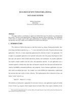
Figure 7: Contour plot generated using a select
* where epoch = 2100 query over a regression-based
view. The variable-sized dots represent the raw data
for that epoch (larger dot size → larger temperature
value).
view structures (e.g., caches). In future we plan to use
the Derby tables for supporting such persistence.
• Predicate pushdown modules (∼ 200 lines): for
analyzing the predicates in a user-posed query, and
pushing them down into the query evaluation mod-
ule; this is much more critical for MauveDB since fine-
granularity model-based views can generate a large
number of tuples if scanned fully.
Our experience with building MauveDB suggests that no
drastic changes to the existing code base are required to
support most model-based views. Moreover much of the
additional code is generic in nature so that supporting new
types of models should require even fewer changes now that

the basic infrastructure is established.
5. PERFORMANCE STUDY
In this section we report the results of an experimental
study over our prototype implementation of MauveDB. We
begin with three examples that demonstrate how the system
works and illustrate the advantages of using MauveDB for
pro ces sing real-world data even with the simple set of mod-
els we have currently implemented. We then present a per-
formance study of the regression- and interpolation-based
mo dels that compares the various view maintenance strate-
gies to each other.
Intel Lab Dataset: For our study, we use the publicly
available Intel Lab dataset [27] that consists of traces from
a 54-node sensor network deployment that measures various
physical attributes such as temperature, humidity etc., us-
ing the Berkeley Motes (sensor nodes) at several locations
within the Intel Research Lab at Berkeley. The need for us-
ing statistical models to pro cess this noisy and incomplete
data has already been noted by several researchers [17, 12].
We use five attributes from this dataset for our experiments:
500 1000 1500 2000 2500
Epoch Number
16
18
20
22
24
Avg temperature
(i) Computed using raw data
500 1000 1500 2000 2500

Epoch Number
16
18
20
22
24
Avg temperature
(ii) Computed using interpolation-based view
500 1000 1500 2000 2500
Epoch Number
0
20
40
60
80
100
% of Sensor Reporting
(iii) % of Sensors Reporting
Figure 8: Results of running select avg(temp) group by epoch (i) over the raw data, and (ii) over the
interpolation-based view. (iii) shows the percentage of sensors reporting at each epoch.
(1) epoch number, a monotonically increasing variable that
records the (discrete) time instance at which a reading was
taken, (2) sensorid, (3) x-coordinate, and (4) y-coordinate
of the sensor making the measurement, and (5) temperature
recorded by the sensor. The dimensions of the lab are 40
meters by 30 meters.
All the exp e riments were carried out on a 1.33 GHz Pow-
erPC G4 with 1.25GB of memory, running Mac OS X.
5.1 Illustrative Examples
Example 1: For our first example query, we show an instan-

tiation of a regression-based view over the lab dataset that
fits a separate regression function per epoch (time step) us-
ing the x and y coordinates as the independent variables.
The view was created using a command similar to the one
shown in Figure 6(i). Figure 7 shows a contour plot of the
temp erature over the whole lab at epoch 2100 using the re-
gression function. The data for generating this contour plot
was obtained by running a simple select query over the
view. The result is a smooth function that provides a rea-
sonable estimate of the temperature throughout the lab –
this is clearly much more informative and useful than the
original data that was generated at that epoch. Though we
could have done this regression by importing the data into
Matlab this would b e considerably slower (as we discuss be-
low) and would not have allowed us to run SQL queries over
the resulting model output.
Example 2: For our second example query, we show an in-
stantiation of an interpolation-based view that linearly in-
terp olates the lab data at each sensor separately (Figure
6(ii)). This allows us to systematically handle data that
might be missing from the dataset (as Figure 8 (iii) shows,
readings from about 40% of the sensors are typically miss-
ing at each epoch). Figures 8 (i) and 8 (ii) show the results
of running a select avg(temp) group by epoch que ry over
both the raw data and the interpolation-based view. Notice
that the first graph is very jittery as a result of the missing
data, whereas the second graph is smoother and hence sig-
nificantly more useful. For example, if this data were being
fed to a control system that regulated temperature in the
lab, using the raw data directly might result in the A/C or

the heater being turned on and off much more frequently
than is needed.
Example 3: Figure 9 shows a natural query that a user might
want to ask on the Intel Lab Dataset that looks for the pairs
of sensors that almost always return results close to each
other. Unfortunately, because of the amount of missing data
in this dataset, this query returns zero results over the raw
dataset. On the other hand, when we ran this query against
the Interpolation-based view defined above, the query re-
turned 57 pairs of sensors (∼ 4% of total pairs).
The above illustrative examples clearly demonstrate the
need for model-based views when dealing with data collected
from sensor networks, since they allow us to pose meaningful
queries despite noise and loss in the underlying data.
select t1.sensorid, t2.sensorid, count(*)
from datatable t1, datatable t2
where abs(t1.temp - t2.temp) < 0.2
and t1.epoch = t2.epoch
and t1.sensorid < t2.sensorid
group by t1.sensorid, t2.sensorid
havin g count(*) > 0.95 * (select
count(distinct epoch) from datatable);
Figure 9: A complex query for finding the sensors
that almost always report temperature close to each
other. datatable can be either the raw table or the
interpolation-based view.
5.2 Comparing View Maintenance Strategies
We have implemented the four view maintenance strate-
gies proposed in Section 3.3.2 for the two kinds of views that
MauveDB currently supports.

• From Scratch (FROMSCRATCH): In this naive
strategy, the raw data is read, and the model built only
when a query is posed against the view.
• Using an Intermediate Representation (COEFF):
MauveDB supports two intermediate query process-
ing options, (1) materializing the sufficient statistics
for regression-based views, and (2) building trees for
interpolation-based views (Section 3.3.2).
• Lazy Materialization (LAZY): This caching-based
approach opportunistically caches the parts of the views
that have been computed in response to a query. The
caches are invalidated when new tuples arrive.
• Forced Materialization (FORCE): Analogous to
materialized views, this option always keeps a model-
based view materialized. Thus when a new raw data
tuple arrives in the system, the view, or a part of it, is
recomputed as required.
Inserts Point Queries Average Queries
50
100
150
Total Time (s)
(i) Regression, per Sensor
FromScratch
Coeff
Lazy
Force
Inserts Point Queries Average Queries
20
40

60
80
Total Time (s)
(ii) Interpolation, per Sensor
Inserts Point Queries Average Queries
10
20
30
40
50
Total Time (s)
(iii) Regression, per Epoch
112.4 s
Figure 10: Comparing the view maintenance strategies for the three
model-based views
10m x 10m 5m x 5m 1m x 1m 0.5m x 0.5m
View Granularity
0
20
40
60
80
Total Insert Time (s)
Coeff
Force
Figure 11: Effect of view gran-
ularity on insert performance
We show results from three different model-based views
that have differing characteristics:
• Regression view per sensor: A different regression

function is fit per sensor. Thus, internally, there will
be 54 separate views created for this overall view.
• Interpolation view per sensor: Similarly, the data
at each sensor is interpolated separately.
• Regression view per epoch: A different regression
function is fit per epoch. Though this results in a larger
number of separate views being created, the opportu-
nities for caching/materialization are much better be-
cause of the monotonicity of time (i.e., once values for
a particular time have been inserted, new values do
not arrive.) The granularity of the view is set to 5m.
To simulate continuous arrival of data tuples and snap-
shot queries posed against the view, we start with a raw
table that already contains 50000 records, and show the re-
sults from the next 1000 tuple inserts, uniformly interleaved
with 50 point queries asking for the temperature at a specific
lo cation at a specific time, and 10 average queries that com-
pute the average temperature with a group by on location
over the entire history. All reported numbers are averages
over 5 runs each.
Figure 10 shows the results from these experiments. As
expected, the FROMSCRATCH option rarely does well (ex-
cept for inserts), in some cases resulting in an order of mag-
nitude slowdown. Surprisingly, the LAZY option also does
not do well for any of the queries (except point queries for the
third view). Though it might seem that this query mix is a
best case scenario for LAZY, that is not actually the case, as
the frequent invalidations result in significantly worse per-
formance than the other options. Most surprisingly, FROM-
SCRATCH outperforms LAZY in some cases, as a result of

the (wasted) extra cost that LAZY pays for caching tuples.
Surprisingly, FORCE performs well in most cases, except
for its insert performance on the first view, which is orders
of magnitude worse than the other options. This is because
re-computation of this view is expensive, and FORCE does
far more re-computations than the other approaches. Not
surprisingly, COEFF performs best in most scenarios. How-
ever, as these experiments show, there are some cases where
one of other options, especially FORCE, may be preferable.
Figure 11 compares the insert performance of COEFF
and FORCE as the granularity of the third view (Regres-
sion, per Ep och) is increased from 10m ×10m to .5m × .5m.
As expected, the performance of COEFF is not affected by
the granularity of the view, but the performance of FORCE
degrades drastically for fine-granularity views, because of
the larger size of the view, suggesting that FORCE should
be avoided in such cases. Choosing which query process-
ing option to use for a given view type and a given query
workload will be a major focus of our future research.
As a point of comparison, we measured the amount of time
required to extract 50,000 records from a raw data table
in Derby using Matlab, fit those readings to a regression
function, and then answer a point or average query. The
time breakdown for these various options is as follows:
Operation Time
Load 50,000 Readings via JDBC 12.05 s
Perform linear regression 1.42 s
Answer an average query 5 ms
Table 1: Time to perform regression in Matlab.
If we wanted to re-learn this model for each of the 1,000

inserts, this process would take about 13,740 seconds in Mat-
lab; if we instead used a lazy approach where we only rebuilt
the model before one of the 60 queries, the total time would
be 808 seconds. The total code to do this in Matlab is about
50 lines of code and took us about four hours write; if we
wanted to write a new query or use a different model, much
of this code would have to be re-written from scratch (par-
ticularly since regression is easy to code in Matlab as it is
included as a fundamental operator). Hence, MauveDB of-
fers a significant performance and usability gain over the
traditional approach used by scientists and engineers today.
6. EXTENSIONS AND FUTURE WORK
We briefly discuss some of the most interesting directions
in which we are planning to extend this research.
Dynamic Probabilistic Model-based Views: As we
discussed briefly in Section 2.2.3, dynamic probabilistic mod-
els (e.g., Kalman Filters) are commonly used to filter real-
world measured data. Figure 12 shows the view creation
syntax that we are investigating for creating a Kalman Filter-
based view. As we can see, this is fairly similar to the view
creation statements we saw earlier, the main difference be-
ing the observations clause that is used to specify the data
to be filtered. We are also investigating other options (e.g.,
PMML) for defining such views. These types of views also
generate probabilistic data that may exhibit very strong cor-
relations raising interesting query processing challenges.
APIs for supporting arbitrary models: Given the di-
create view KFView(t[0::1],sensorid[::1],temp)
as KalmanFilter for each sensorid M
training data select * from raw-temp-readings

where raw-temp-readings.sensorid = M and time
between training-start and training-end
observations select * from raw-temp-readings
where raw-temp-readings.sensorid = M and
time > training-end
Figure 12: Specifying a Kalman Filter-based View
versity in the commonly used statistical and probabilistic
mo dels, it is challenging for a single system like MauveDB to
support every such model. Our hypothesis, however, is that
the interface between most models and the database system
can be encapsulated using a small set of functions. Develop-
ing this generic API for adding new models to MauveDB is
one of the most important tasks in this area.
Continuous Queries: Since the sensor data is generated
and processed in real-time, we expect users to desire support
for continuous queries. There has been much work on con-
tinuous query processing over data streams in recent years;
the complex interactions between s uch queries and model-
based views, however, pose many research challenges that
have not been studied before. Language extensions that
can support both continuous queries as well as probabilis-
tic queries (for handling probabilistic views discussed above)
also remains an open problem.
Active Data Acquisition: By their very nature, distributed
measurement systems need to control how, where, and with
what frequency the data is acquired, the chief reason be-
ing that the system will otherwise be inundated with huge
amounts of redundant and useless information. [12] dis-
cusses how probabilistic models can be used to control data
acquisition in sensor networks. Supporting such data acqui-

sition seamlessly in our system is an interesting challenge
that we plan tackle in future.
7. RELATED WORK
Database Views: Views have been a mainstay of data
management systems from the early days of relational sys-
tems, and are used to both make it easier for users to access
the data, and to restrict what users can access [11]. There
is a rich literature that addresses various aspects such as
definitions of views, compositions of views, materialization
of views, maintenance of materialized views, and answer-
ing queries over views (see, e.g., [18], for an overview of
these techniques). To our knowledge, ours is the first work
that furthers the abstraction of views by allowing views to
be defined using complex statistical models instead of SQL
queries, raising new and unique challenges that have not
been studied before.
Data Mining: Data mining has traditionally been the
playground for cross-disciplinary research between machine
learning and database systems. Though there has been
much work in this area [19], to our knowledge, none of it has
attempted to fundamentally change the user view of the un-
derlying data through use of statistical models. PMML [33]
is a modeling language designed to describe statistical mo d-
els and their parameters – for example, PMML can be used
to describe the parameters of a set of basis functions that fit
a particular data set. There are various modeling tools (e.g.,
IBM’s Intelligent Miner [20]) that can learn and output such
mo dels, as well as some databases (such as DB2) that can
use PMML models as user-defined functions. Sarawagi et
al. [34] and Chaudhuri et al. [7] present more sophisticated

schemes than those supported by commercial tools for effi-
ciently operating over previously learned models inside of a
database system. None of these approaches, however, pro-
vide support for updating the parameters of models inside of
the database system, limiting their applicability in scientific
environments where new data is continually arriving.
There are also various commercial tools for data mining
that sit on top of a database. Perhaps the most widely used
are the SAS Analytics tools [35], though scientists and engi-
neers frequently use Matlab, Maple, or other such packages.
As discussed above, though these tools are powerful, the fact
that they are not integrated into the database system limit
their performance and usability.
Probabilistic/Incomplete Data Management: There
has also been much work on managing probabilistic, impre-
cise, incomplete or fuzzy data in database systems (e.g., [24,
4, 25, 21, 15, 13, 10, 36]). With an increasing need for sys-
tems to manage real-world data that often tends to be noisy,
incomplete and uncertain, there has been a renewed interest
in this area in recent years. This interest has also been fu-
eled by a growth in other application domains such as data
integration where uncertain data with probabilities attached
to tuples arises naturally [13, 10, 2]. Several research efforts
are underway to build systems to manage uncertain data
(e.g. MYSTIQ [10], Trio [36], ORION [8, 37], ConQuer [2]).
None of this work, however, proposes to use statistical mod-
els as the fundamental abstraction presented to the users.
Neugebauer [31] presents a scheme for performing inter-
polation inside a database system that is similar in spirit
to MauveDB, including query language extensions and opti-

mizations for efficient operation inside of the database sys-
tem. Her work does not generalize to other types of models,
however, limiting its use to applications that rely solely on
interpolation. A more thorough treatment of optimizing in-
terp olation queries is presented by Grumbach et al. [16],
though again the focus is solely on interpolative queries.
Wireless Sensor Networks: Wireless sensor networks
have been a very active area of research in recent years
(see [1] for a survey). There is a large body of work on
data collection from sensor networks that applies higher-
level techniques to sensor network data processing. Directed
diffusion [22] is a general purpose data collection mechanism
that uses a data-centric approach to disseminate queries and
gather data. Cougar and TinyDB [38, 28] provide declara-
tive interfaces to acquiring data from sensor networks. Sev-
eral systems propose to use probabilistic modeling tech-
niques to answer queries over sensor networks [23, 12, 9],
though these have typically used specific models rather
than generalized implementation in an existing relational
database as in MauveDB.
8. CONCLUSIONS
In this paper, we presented the architecture of MauveDB,
a data management system that fundamentally integrates
statistical models into database systems by providing a new
abstraction called model-based views. Model-based views
further the classic notion of “data independence” by insulat-
ing the users from the messy details of underlying real-world
data; they achieve this by allowing users to specify statis-
tical models to be applied to the data inside the database
system, and thereby always presenting the users with a con-

sistent view of the data or the system being monitored.
We are in the process of building MauveDB using the
Apache Derby open-source database system, and our cur-
rent prototype not only allows users to specify and create
mo del-based views over raw data tables using two commonly
used statistical modeling techniques (namely, regression and
interpolation), but also provides transparent support for
querying such views using SQL, and for keeping them up-
to-date as new tuples arrive. Our experimental study shows
that model-based views can significantly improve the user
interaction with real-world data, by allowing natural user
queries to return meaningful results, and by removing noise
from the returned answers. We also propose and experiment
with four different view maintenance strategies, and our ex-
perimental results suggest that keeping an intermediate rep-
resentation of the views provides the best performance.
9. REFERENCES
[1] I.F. Akyildiz, W. Su, Y. Sankarasubramaniam, and
E. Cayirci. Wireless sensor networks: a survey.
Computer Networks, 38, 2002.
[2] Periklis Andritsos, Ariel Fuxman, and Renee J. Miller.
Clean answers over dirty databases. In ICDE, 2006.
[3] The Apache Derby Project. Web Site.
/>[4] D. Barbara, H. Garcia-Molina, and D. Porter. The
management of probabilistic data. IEEE TKDE,
4(5):487–502, 1992.
[5] Tim Brooke and Jenna Burrell. From ethnography to
design in a vineyard. In Proceeedings of the Design
User Experiences (DUX) Conference, June 2003.
[6] A. Cerpa, J. Elson, D.Estrin, L. Girod, M. Hamilton,

and J. Zhao. Habitat monitoring: Application driver
for wireless communications technology. In Proceedings
of ACM SIGCOMM 2001 Workshop on Data
Communications in Latin America and the Caribbean.
[7] Surajit Chaudhuri, Vivek Narasayya, and Sunita
Sarawagi. Efficient evaluation of queries with mining
predicates. In Proceedings of ICDE, 2002.
[8] Reynold Cheng, Dmitri V. Kalashnikov, and Sunil
Prabhakar. Evaluating probabilistic queries over
imprecise data. In Proceedings of SIGMOD, 2003.
[9] M. Chu, H. Haussecker, and F. Zhao. Scalable
information-driven sensor querying and routing for ad
hoc heterogeneous sensor networks. In Intl Journal of
High Performance Computing Applications, 2002.
[10] Nilesh N. Dalvi and Dan Suciu. Efficient query
evaluation on probabilistic databases. In VLDB, 2004.
[11] Dorothy E. Denning et al. Views for multilevel
database security. IEEE Trans. Softw. Eng., 1987.
[12] Amol Deshpande, Carlos Guestrin, Sam Madden, Joe
Hellerstein, and Wei Hong. Model-driven data
acquisition in sensor networks. In VLDB, 2004.
[13] Norb ert Fuhr and Thomas Rolleke. A probabilistic
relational algebra for the integration of information
retrieval and database systems. ACM Trans. Inf.
Syst., 15(1):32–66, 1997.
[14] G. Golub and C. Van Loan. Matrix Computations.
Johns Hopkins, 1989.
[15] G. Grahne. Horn tables - an efficient tool for handling
incomplete information in databases. In PODS, 1989.
[16] S. Grumbach, P. Rigaux, and L. Segoufin.

Manipulating interpolated data is easier than you
thought. In VLDB, 2000.
[17] C. Guestrin, P. Bodik, R. Thibaux, M. Paskin, and
S. Madden. Distributed regression: an efficient frame-
work for modeling sensor network data. In IPSN, 2004.
[18] A. Gupta and I.S. Mumick. Materialized views:
techniques, implementations, and applications. MIT
Press, 1999.
[19] David Hand, Heikki Mannila, and Padhraic Smyth.
Principles of Data Mining. MIT Press, 2001.
[20] DB2 Intelligent Miner. Web Site.
/>[21] T. Imielinski and W. Lipski Jr. Incomplete infor-
mation in relational databases. JACM, 31(4), 1984.
[22] C. Intanagonwiwat, R. Govindan, and D. Estrin.
Directed diffusion: A scalable and robust
communication paradigm for sensor networks. In
MOBICOM, 2000.
[23] A. Jain, E. Change, and Y. Wang. Adaptive stream
resource management using kalman filters. In
SIGMOD, 2004.
[24] L. V. S. Lakshmanan, N. Leone, R. Ross, and V. S.
Subrahmanian. Probview: a flexible probabilistic
database system. ACM TODS, 22(3), 1997.
[25] Suk Kyoon Lee. An extended relational database
mo del for uncertain and imprecise information. In
VLDB, 1992.
[26] L. Liao, D. Fox, and H. Kautz. Location-based
activity recognition using relational markov networks.
In IJCAI, 2005.
[27] Sam Madden. Intel lab data, 2004.

/>[28] Samuel Madden, Wei Hong, Joseph M. Hellerstein,
and Michael Franklin. TinyDB web page.
/>[29] A. Mainwaring, J. Polastre, R. Szewczyk, and
D. Culler. Wireless sensor networks for habitat
monitoring. In ACM Workshop on Sensor Networks
and Applications, 2002.
[30] Erin McKean, editor. The Oxford English Dictionary
(2nd Edition). Oxford Univeristy Press, 2005.
[31] Leonore Neugebauer. Optimization and evaluation of
database queries including embedded interpolation
procedures. In Proceedings of SIGMOD, 1991.
[32] George M. Phillips. Interpolation and Approximation
by Polynomials. Springer-Ve rlag, 2003.
[33] PMML 3.0 Specification. Web Site.
/>[34] S. Sarawagi, S. Thomas, and R. Agrawal. Integrating
association rule mining with databases: alternatives
and implications. In Proceedings of SIGMOD, 1998.
[35] Business Analytics Software Solutions (SAS). Web
Site. />[36] J. Widom. Trio: A system for integrated management
of data, accuracy, and lineage. In CIDR, 2005.
[37] Y. Xia, S. Prabhakar, S. Lei, R. Cheng, and R. Shah.
Indexing continuously changing data with
mean-variance tree. In ACM SAC, 2005.
[38] Y. Yao and J. Gehrke. Query processing in sensor
networks. In CIDR, 2003.