REED: Robust, Efficient Filtering and Event Detection in Sensor Networks docx

REED: Robust, Efficient Filtering and Event Detection
in Sensor Networks
Daniel J. Abadi, Samuel Madden, and Wolfgang Lindner
MIT CSAIL
{dna, madden, wolfgang}@csail.mit.edu


Abstract
This paper presents a set of algorithms for efficiently
evaluating join queries over static data tables in sen-
sor networks. We describe and evaluate three algo-
rithms that take advantage of distributed join tech-
niques. Our algorithms are capable of running in lim-
ited amounts of RAM, can distribute the storage bur-
den over groups of nodes, and are tolerant to dropped
packets and node failures. REED is thus suitable for
a wide range of event-detection applications that tra-
ditional sensor network database and data collection
systems cannot be used to implement.
1. Introduction
A widely cited application of sensor networks is event-
detection, where a large network of nodes is used to iden-
tify regions or resources that are experiencing some phe-
nomenon of particular concern to the user. Examples in-
clude condition-based maintenance in industrial plants
[14], where engineers are concerned with identifying ma-
chines or processes that are in need of repair or adjustment,
process compliance in food and drug manufacturing [25],
where strict regulatory requirements require companies to
certify that their products did not exceed certain environ-
mental parameters during processing, and applications

centered around homeland security, where shippers are
concerned with verifying that their packages and crates
were not tampered with in some unsavory manner.
A natural approach to implementing such systems is to
use an existing query-based data collection system for sen-
sor networks. Through queries, a user can ask for the data
he or she is interested in without concern for the technical
details of how that data will be retrieved or processed. A
number of research projects, including Cougar [31], Di-
rected Diffusion [12], and TinyDB [19,20] have advocated
a query-based interface to sensornets, and several imple-
mentations of query systems have been built and deployed.
Unfortunately, these existing query systems do not pro-
vide an efficient way to evaluate the complex predicates
these event-detection applications require because they lack
a join operator that would naturally be used to express the
checking of a large number of predicates against the cur-
rent readings of sensors and thus cannot be used in many
condition-based monitoring and compliance applications.
For example, we have been talking with Intel engineers
deploying wireless sensornets for condition based mainte-
nance in Intel’s chip fabrication plants who report that they
have thousands of sensors spread across hundreds of pieces
of equipment that are each involved in a number of differ-
ent manufacturing processes that are characterized by dif-
ferent modes of behavior [13,14].
In this paper, we present REED, a system for Robust and
Efficient Event Detection in sensor networks that addresses
this limitation, enabling the deployment of sensor networks
for the types of applications described above. REED is

based on TinyDB, but extends it with the ability to support
joins between sensor data and static tables built outside the
sensor network. This allows users to express queries that
include complex time and location varying predicates over
any number of conditions using join predicates over these
different attributes. The key idea behind REED is to store
filter conditions in tables, and then to distribute those tables
throughout the network. Once these tables have been dis-
seminated, each node joins the filters to its readings by
checking each tuple of readings it produces against all of
the predicates, outputting a list of predicates that the tuple
satisfies. This list of satisfying predicates is then transmit-
ted out of the network to inform the user of conditions of
interest. Though this process is logically similar to a stan-
dard relational join, we show that join processing in sensor
networks introduces a substantial set of new architectural
challenges and optimization opportunities.
By performing this join in-network, REED can dramati-
cally reduce the communications burden on the network
topology, especially when there are relatively few satisfy-
ing tuples, as is typically the case when identifying failures
in condition-based monitoring or process compliance ap-
plications. Reducing communication in this way is particu-
larly important in many industrial scenarios when relatively
high data rate sampling (e.g., 100’s of Hertz) is required to
perform the requisite monitoring [10]. Table 1 shows an
example of the kinds of tables which we expect to transmit
– in this case, the filtration predicates vary with time, and
include conditions on both the temperature and humidity.
Our discussions with various commercial companies (e.g.,

Honeywell and ABB) involved in process control suggest
that these kinds of predicates are representative of many
sensor-based monitoring deployments in the real world.
Interestingly, both TinyDB [19] and Cougar [31] ini-
tially eschewed joins in their query languages as their au-
thors believed joins were of limited utility; REED provides
an excellent counter-example to this point of view. In fact,
we have added support for joins between external tables
Permission to copy without fee all or part of this material is granted
provided that the copies are not made or distributed for direct commer-
cial advantage, the VLDB copyright notice and the title of the publica-
tion and its date appear, and notice is given that copying is by permis-
sion of the Very Large Data Base Endowment. To copy otherwise, or to
republish, requires a fee and/or special permission from the Endow-
ment.
Proceedings of the 31st VLDB Conference,
Trondheim, Norway, 2005
and sensor readings to TinyDB; users can now write que-
ries of the form:

SELECT s.nodeid, a.condition_type
FROM sensors AS s, alert_table AS a
WHERE s.temp > a.temp_thresh
AND s.humidity > a.humid_thresh
AND s.time = a. time
SAMPLE PERIOD 1s
Here, we use TinyDB syntax, where sensors refers to
the live sensors readings (produced once per second, in this
case). In REED, the external alert_table (similar, for
example, to Table 1) will be pushed into the network along

with the query. The filter conditions will be evaluated by
having each node join the sensors tuples that it produces
with the conditions in the table, with matches producing
tuples of the form <nodeid, condition_type> that
are then transmitted to the user.
Because storage on sensor network devices is typically
at a premium (e.g., Berkeley motes have just a few kilo-
bytes of RAM and half a megabyte of Flash), REED allows
these predicate tables to be partitioned and stored across
several sensors. It also can transmit just a fragment of the
predicate table into the network, forcing readings which do
not have entries in the table to be transmitted out of the
network and joined externally. REED attempts to deter-
mine which predicates are most important to send into the
network based on historical observations of predicates
which commonly are not satisfied.
Finally, to facilitate the integration with external data-
bases, we have integrated REED into the Borealis stream
processing engine [3]. This allows us to issue queries at a
centralized processor, which extracts relevant selection
predicates and joins and pushes them into the network
when the optimizer believes such push-down will be help-
ful.
1.1. Contributions
In summary, the major contributions of this work are:
• We show how complex filters can be expressed as
tables of conditions, and show that those conditions
can be evaluated using relational join operations.
• We describe the REED system and our sensor network
filtration algorithms, which are tailored to provide ro-

bustness in the face of network loss and to handle very
limited memory resources.
• We provide experimental results showing the substan-
tial performance advantages that can be obtained by
executing complex join-based filters inside the sensor
network, through evaluation in both simulation and on
a real, mote-based sensor network.
• We discuss a number of variants and optimizations of
our approach, some of which are motivated by join op-
timizations in traditional databases and others which
we have developed to address the particular properties
of sensor networks.
• We describe our initial integration of REED and Bore-
alis and show an example illustrating how Borealis can
push join operators into the sensornet.
Before describing the details of our approach, we briefly
review the syntax and semantics of sensor network queries
and the capabilities of current generation sensornet hard-
ware.
2. Background: Sensor Networks and Motes
Sensor networks typically consist of tens to hundreds of
small, battery-powered, radio-equipped nodes. These
nodes usually have a small, embedded microprocessor,
running at a few Mhz, with a small quantity of RAM and a
larger Flash memory. The Berkeley mica2 Mote is a popu-
lar sensor network hardware platform designed at UC
Berkeley and sold commercially by Crossbow Corporation.
It has a 7 Mhz processor, a 38.6Kbps radio with ~100 foot
range, 4KB of RAM and 512KB flash, runs on AA batter-
ies and uses ~15 mA in active power consumption and ~10

µA when asleep.
Storage: The limited quantities of memory are of particular
concern for query processing, as they severely limit the
sizes of join and other intermediate result tables. Although
future generations of devices will certainly have somewhat
more RAM, large quantities of RAM are problematic be-
cause of their high power consumption. Non-volatile flash
can make up for RAM shortages to some extent, but flash
writes are quite slow (several milliseconds per page, with
typical pages less than 1 KB) and consume large amounts
of energy – almost as much as transmitting data off of the
mote [28]. Hence, memory efficient algorithms are criti-
cally important in sensornets.
Sensors: Mica2 motes include a 51-pin expansion slot that
accommodates sensor boards. Commonly available sen-
sors measure light, temperature, humidity, vibration, accel-
eration, and position (via GPS or ultrasound).
Communication: Radio communication tends to be quite
lossy – without retransmission, motes drop significant
numbers of packets. At very short ranges, loss rates may
be as low as 5%; at longer ranges, these rates can climb to
50% or more [30]. Though retransmission can mitigate
these losses somewhat, nodes can still fail, move away, or
be subject to radio interference that makes them temporar-
ily unable to communicate with some or all of their
neighbors. Thus, any algorithm that runs inside of a sensor
network must tolerate and adapt to some degree of com-
munication failure.
TinyOS: Motes run a basic operating system called
TinyOS [12], which provides a suite of software libraries

for sending and receiving messages, organizing motes into
ad-hoc, multihop routing trees, storing data to and from
flash, and acquiring data from sensors.
Power: Because sensors are battery powered, power con-
sumption is of utmost concern to application designers.
Power is consumed by a number of factors; typically, sens-
ing and communicating dominate this cost [19,24]. In this
paper, we focus on algorithms that minimize communica-
Table 1: Example of a Table of Predicates used in Con-
dition-based Monitoring
Condition # Time Temp_thresh Humid_thresh
1 9 pm
> 100° C
> 95 %
2 10 pm
> 110° C
> 90 %
3 11 pm
> 115° C
> 87 %
… … … …
tion, as any join algorithm that includes all nodes in a net-
work will pay the same cost for running sensors. We note
that if careful power management is not used, the cost of
listening to the radio will actually dominate the cost of
transmitting, as sending a message takes only a few milli-
seconds, but the receiver may need to be on continuously,
waiting for a message to arrive. TinyDB and TinyOS ad-
dress this issue by using a technique called low-power lis-
tening [23].

2.1. Background: Data Model and Semantics
REED adopts the same data model and query semantics as
TinyDB. Queries in TinyDB, as in SQL, consist of a SE-
LECT-FROM-WHERE clause supporting selection, projec-
tion, and aggregation. REED extends this list of operators
with joins. TinyDB treats sensor data as a single table
(sensors) with one column per sensor type. Results, or
tuples, are appended to this table periodically, at well-
defined intervals that are a parameter of the query, speci-
fied in the SAMPLE PERIOD clause. The period of time
from the start of each sample interval to the start of the next
is known as an epoch. Consider the query:
SELECT nodeid, light, temp
FROM sensors
SAMPLE PERIOD 1s FOR 10s
This query specifies that each sensor should report its own
id, light, and temperature readings once per second for ten
seconds. Thus, each epoch is one second long.
2.2. Data Collection in TinyDB
Query processing in the original TinyDB implementation
works as follows. The query is input on the user’s PC, or
basestation. This query is optimized to improve execution;
currently, TinyDB only considers the order of selection
predicates during optimization (as the existing version does
not support joins). Once optimized, the query is translated
into a sensor-network specific format and injected into the
network via a gateway node. The query is sent to all nodes
in the network using a simple broadcast flood (TinyDB
also implements a form of epidemic query sharing which
we do not discuss).

As the query is propagated, nodes learn about their
neighbors and assemble into a routing tree; in TinyDB, this
is implemented using a standard TinyOS service similar to
what is described in the work by Woo et al. [30]. Each
node in the network picks one node as its parent that is one
network hop closer to the root than it is. A node’s depth is
simply the number of radio hops required for a message it
sends to reach the basestation.
As a node produces query answers, it sends them to its
parent; in turn, parents forward data to their parents, until
answers eventually reach the root. For some queries (and
in our join implementation), parents will combine readings
from children with local data to partially process queries
within the network. The basestation assembles partial re-
sults from nodes in the network, completes query process-
ing, and displays results to the user.



3. Applications and Query Classification
In this section, we describe some applications of REED.
We use these applications to derive a classification of joins
that motivate the join algorithms presented in Section 4.
3.1. Query Types
REED extends the query language of TinyDB by allowing
tables of filter predicates to appear in the FROM clause. In
this section, we show the syntax of several example queries
and describe their basic behavior.
Industrial Process Control. Chemical and industrial
manufacturing processes often require temperature, humid-

ity, and other environmental parameters to remain in a
small, fixed range that varies over time [11]. Should the
temperature fall outside this range, manufacturers risk
costly failures that must be avoided. Thus, they currently
employ a range of wired sensing to avoid such problems
[25,13]. Interestingly, companies in this area (e.g., GE,
Honeywell, Rockwell, ABB, and others) are aggressively
pursuing the use of mote-like devices to provide wireless
connectivity, which is cheaper and safer than powered so-
lutions as motes don’t require expensive wires to be in-
stalled and avoid the risks associated with running high-
voltage wires through volatile areas. Of course, for wire-
less solutions to be cost-effective, they must provide many
months of battery life as well as equivalent levels of infor-
mation to existing solutions. Thus, the power and commu-
nications efficiency of a system like REED is potentially of
great interest.
It is easy to write a REED query that filters readings
from sensors located at various positions with a time-
indexed table of predicates that encodes, for example, al-
lowable temperature ranges in a process control setting.
Should the temperature ever fall outside the required range,
users can be alerted and appropriate action can be taken.
Such a query might look like:

(1)
SELECT a.atemp
FROM schedule_table AS t,
sensors AS a
WHERE a.ts > t.tsmin AND

a.ts < t.tsmax AND
a.atemp > t.tempmin AND
a.atemp < t.tempmax AND
a.nodeid = t.nodeid
Here, results are produced only when an exceptional
condition is reached (the temperature is outside the desired
range), and thus relatively few tuples will match. We note
that this is a low selectivity query, indicating that it outputs
(selects) a small percentage of the original sensor tuples.
As mentioned above, our discussions with engineers in
industrial settings suggest that each sensor may have sev-
eral alarm conditions associated with it, and there may be
hundreds or thousands of sensors in a single factory. In a
typical deployment such as Intel’s, there could be several
thousand filters, each of which consists of a time range, a
minimum and maximum sensor value, and a node id. Sup-
posing these numbers require 16 bytes to store, the total
join table in the case of the Intel deployment might be
100KB or larger.
Failure and Outlier Detection. One of the difficulties
of maintaining a large network of battery-powered, wire-
less nodes is that failures are frequent. Sometimes these
failures are fail-fast: for example, a node’s battery dies and
it stops reporting readings. At other times, however, these
failures are more insidious: a node’s readings slowly drift
away from those of sensors around it, until they are mean-
ingless or useless. Of course, there are times when such
de-correlated readings actually represent an interesting,
highly localized event (i.e., an outlier). In either case,
however, the user will typically want to be informed about

the readings. We have implemented a basic application
that performs both these tasks in REED. It works as fol-
lows: we build a list of the values that each node com-
monly produces during particular times of day from his-
torical data and periodically update this list over time. We
then use this list to derive a set of low-probability value
ranges that never occur or that occur with some threshold
probability ε or less frequently. Then, we run a query
which detects these unusual values. For example, the fol-
lowing query detects outlier temperatures:

SELECT s.nodeid, s.temp
FROM sensors AS s, outlier_temp AS o
WHERE s.temp
BETWEEN o.low_temp AND o.hi_temp
AND s.roomno = a.roomno

This query reports all of the readings that are within an
outlier range in a given room number. Note that the out-
lier_temp table may be quite large in this case, but that
the selectivity of this query is also low.
Power Scheduling. As a third example, consider a set
of sensors in a remote environment where power conserva-
tion is of critical importance. To minimize power consump-
tion in such scenarios, it is desirable to balance work across
a group of sensors where each sensor only transmits its
light reading some small fraction of the time. We can do
this with an external table as well; for example:

SELECT sensors.nodeid, sensors.light

FROM sensors, roundrobin
WHERE sensors.nodeid = roundrobin.nodeid
AND sensors.ts % |nodes| = roundrobin.ts

For this query, the roundrobin table is small (≤
|nodes| entries), and can likely fit on one node. This filter
also has a low selectivity, as only one or two nodes satisfy
the predicate per time step.
3.2. Query Classes and Optimizer Tradeoffs
These queries allow us to make several observations about
how and where we should execute joins. In general, it is
advantageous to perform joins with low selectivity in the
sensor network. This is because there will be many fewer
results than original data and thus a smaller number of
transmissions needed to get data to the basestation.
There are situations, however, when we might prefer not
to push a join into the network; for example, if the join has
a relatively high selectivity, and the size of the predicate
table is very large, the cost of sending the join into the net-
work may exceed the benefit of applying the join inside the
network. We may also be unable to push a join into the
network if the size of the predicate table exceeds the stor-
age of a single node or a group of nodes across which the
table may be partitioned.
Thus, in REED, we differentiate between the following
types of joins:
- Small join tables that fit in the RAM of a single node.
- Intermediate join tables that exceed the memory of a
single node, but can fit in the aggregate memory of a
small group of nodes.

- Large join tables that exceed the aggregate memory of a
group of nodes.
We have developed join algorithms that are suitable for
all three classes of tables; we describe these algorithms in
Sections 3 and 4 below.
For small join tables, REED always chooses to push
them into the network if their selectivity is smaller than
one. For intermediate tables, the REED query optimizer
makes a decision as to whether to push the join into the
network based on the estimated selectivity of the predicate
(which may be learned from past performance or gathered
statistics, or estimated using basic query optimization tech-
niques [28]) and the average depth of sensor nodes in the
network. It uses a novel algorithm to store several copies
of the join table at different groups of neighboring nodes in
the network, sending each sensor tuple to one of the groups
for in-network filtration.
For large joins, as well as intermediate joins that REED
chooses not to place in-network, REED can employ a third
set of algorithms that send a subset of the join table into the
network. REED tags this subset with a logical predicate
that defines which sensor readings it can filter in-network.
For example, for Query (1) above, a join-table subset might
be tagged with a predicate indicating it is valid for nodes 1-
5 at times between 5 am and 5 pm. For readings from these
nodes in this time period, joins can be applied in-network;
other readings will have to be transmitted out of the net-
work and joined externally. We describe algorithms for
these kinds of partial joins in Section 5. If REED chooses
not to apply partial joins, all nodes transmit their readings

out of the network where they are joined externally.
In the following section, we present two algorithms: the
first is a single-node algorithm for small join tables. The
second shows how to generalize this single-node technique
to a group of nodes that work together to collectively store
the filter table. We show that these algorithms are robust to
failures and changes in topology as well as efficient in
terms of communication and processing costs.
4. Basic Join Algorithms
Once the query optimizer has decided to push a REED
query into the network, we need an algorithm for applying
our joins efficiently; in this section, we describe our ap-
proach for performing this computation. We focus on dis-
tributing and executing our filters throughout the network
in a power-efficient manner that is robust in the face of
dropped packets and failed nodes. Logically, our algo-
rithms can be thought of as a nested-loops join between
current sensor readings and a table of static predicates.
Nested-loops joins are straightforward to implement in a
sensornet, as shown by the following algorithm:

Join(Predicate q)
for each tuple t
r
in sensors do
for each tuple t
s
in predicates do
if q(t
r

, t
s
) is satisfied
add t
r
∪ t
s
to result set r
return r
There are two things to note about this algorithm. First,
low selectivity filters might cause there to be fewer than
one result (on average) per element of the outer loop,
though it is in general possible for each tuple to match with
more than one predicate. As in any database system with
these properties, it is advantageous to apply our filters as
close as possible to the data source in a sensor network
since this would reduce the total number of data transmis-
sions in the network. Second, elements of predicates are
independent of each other. Thus, predicates can be hori-
zontally partitioned into a number of non-overlapping sub-
tables, each of which can be placed on separate nodes. As
long as the table partitions are disjoint, the union of the
results of the filter on the independent nodes storing parti-
tions of the table is equal to the results of the filter if the
entire static table was stored at one location.
These two observations motivate our algorithms. The
join is applied as close as possible to the data source. For
the case where the static table fits on one sensor node, the
static table is sent to every sensor node (using the TinyDB
query flood mechanism) and the filter is performed on a

sensor node as soon as the data is produced. For the case
where the static table does not fit on one node, the predi-
cates table (s) is horizontally partitioned into n disjoint
segments s
1
, s
2
, …, s
n
(s=s
1
∪s
2
∪…∪s
n
). Each s
i
is sent to a
member of a group of sensor nodes in close proximity to
each other formed specially to apply the join. Each group is
sent a copy of the predicates table. When a sensor data
tuple is generated, it is sent to each node in exactly one of
these groups to join with every partition (s
i
) of the predi-
cate table.
In Section 4.1 we describe in more detail the case where
the predicates table fits on one node. In Section 4.2, we
extend this basic algorithm with a distributed version for
the case where the table is too big to fit on one node.

4.1. Single Node Join
Our join algorithm leverages the existing routing tree to
send control messages and tuples between the nodes and
the root. When a query involving a join is received at the
basestation, a message announcing the query is flooded
down to all the nodes. This announcement (actually im-
plemented as a set of messages) is an extended version of
the TinyDB “new query” messages, and includes the
schema of the sensor data tuples, the name, size, and
schema of the join table, the schema of the result tuples,
and a set of expressions that form the join predicate. Upon
receiving the complete set of these messages, every node in
the sensor network knows whether it is participating in the
query (by verifying that it contains the sensors that produce
the fields in the schema) and how many tuples of the join
table can be locally stored (by comparing the size of each
join table tuple with the storage capacity the node is willing
to allocate to the query).
If the node’s storage capacity is sufficient to store the
filter predicates table, the node simply sends a message to
the root, requesting the table and indicating that it intends
to store the entire table locally. The root assumes that there
will likely be other nodes that can also store the entire ta-
ble, so it floods each tuple of the table throughout the sen-
sornet. Once the entire table is received, the node can begin
to perform the join locally, transmitting the join results
Figure 1: REED routing and join tree with group overlays

rather than the original data. Before then, nodes run a na-
ïve join algorithm, where sensor tuples are sent to the root

of the network to be joined externally.
A simple optimization that can be performed is that if
the result of the join consists of more than one tuple, the
node can simply send the original sensor tuple. The join for
this tuple can then be performed at the basestation; this
technique is equivalent to semi-joins [4].
4.2. Distributed Join
In this section, we describe our in-network join algorithm
in detail. Our algorithm consists of three distinct phases:
group formation, table distribution, and query processing.
4.2.1. Algorithm Overview
When the predicates table does not fit on one node, joins
can no longer be performed strictly locally. Instead, the
table must be horizontally partitioned. A tuple can only
immediately join with the local partition at the node and
must be shipped to other nodes to complete the join. Once
the original tuple has reached every node that contains a
partition of the table, it can be dropped and results can be
forwarded to the root. Nodes thus organize themselves into
groups that cumulatively store the entire table, where all
group members are within broadcast range of each other.
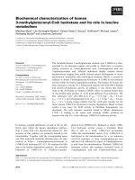
Figure 1 shows the setup of such a distributed join
query. The figure shows a multi-hop routing tree where
tuples are passed to their parents on their path to the root
basestation. For example, a tuple produced by node 7 is
sent to node 5 which then sends the tuple to node 2 which
sends the tuple to the basestation. Our join algorithm works
by overlaying groups (shown as large circles in Figure 1) on
top of this routing tree. The numbers in brackets in the fig-
ure represent the set of nodes in broadcast range for that

particular node. A tuple that needs to be joined is broad-
cast from a node to the other members of its group. Each
member sends any joined results up the original routing
tree. For example, if node 7 produces a tuple to be joined, it
broadcasts it to nodes 5 and 6. If node 5 contains a tuple in
the table that successfully joins with 7’s tuple, it sends the
result up to node 2 which forwards it to the root.
Note that when node 7 produces a tuple that joins with
the static table, three transmissions result; this is the same
as if the original data was sent up the routing tree in the
naïve or single-node case. In the worst case, there would
have been two extra tuples: if node 5 produced a tuple
which joined with a tuple on node 7 a total of 4 transmis-
sions would have been performed. In general, no more
than 2 + depth transmissions will be required, as any pair
of nodes in the same group differ by no more than one level
(by definition). For joins with predicates of low selectivity
there are many cases where no element of the table joins
with the original data. When this occurs, performing the
join in the group rather than sending the tuple back to the
root provides savings proportional to the depth of that
group (instead of n hops to get the data to the root, only 1
transmission of the original data is made).
We now describe the algorithm that each node performs
when it receives a join query with a predicates table whose
size is too large to fit on that node.
4.2.2. Group Formation
If a node calculates that it does not have enough storage
capacity for the table, it initiates the group formation algo-
rithm. To minimize the number of times an original tuple

must be transmitted to make it available to every member
of a group, we require that all nodes in the group are within
broadcast range of each other. A second required property
of a group is that it must have enough cumulative storage
capacity to accommodate the table of predicates. If these
requirements can not be met, the join classification (see
Section 3.2) is not intermediate but rather large, and only
the algorithms described in Section 5 can be used. Group
formation is a background task that happens continuously
throughout the lifetime of the join query as nodes come and
go and network connectivity changes. Every group can be
uniquely identified by its groupid and the queryid.
Every node maintains a global, periodically refreshed
list of neighbors that are within broadcast range. For each
neighbor, an estimate of incoming link quality is computed
by snooping on messages sent by surrounding nodes. A
neighbor node is placed on the neighbor list if the receive
percentage is above some threshold (defaulting to 75%).
This snooping algorithm we use is similar to the algorithm
used for measuring link quality in the TinyOS multihop
radio stack [30].
We give a brief overview of a group formation algo-
rithm here, and refer the reader to our technical report [1]
for a more detailed account of how the algorithm works. It
is important to note that there exist multiple variations on
the algorithm we present; for example, while we do not
allow a node to belong to more than one group, there is no
fundamental reason why this is not possible and in fact this
might allow for fewer copies of the static table to be sent
into the network, optimizing table dissemination costs.

Since our experimental results (Section 6.1.1) show that the
group formation overhead is negligible compared to other
communication required by the query, optimizations on the
group formation algorithm should focus on maximizing the
number of nodes that are members of a group, rather than
trying to minimize the number of messages required to
form a group.
A master node initiates the creation of a group by send-
ing out an announcement and nodes within broadcast range
respond with their neighbor lists and capacities. The master
then attempts to take an intersection of neighbor lists (ac-
counting for asymmetric links in the process) of a subset of
nodes from which it has heard, such that the resulting set of
nodes have enough capacity to store the original table. If
such an intersection exists, the master contacts the root
node and the table is partitioned and distributed evenly
across the nodes in the group (taking into consideration
space constraints on individual nodes). A node moves
through phases in this algorithm by transitioning through
states in a finite state machine which is shown in Figure 2.
4.2.3. Message Loss and Node Failure
The group formation algorithm deals with message loss
by allowing every state in the finite state machine to time
out while having a minimal effect on other nodes. For ex-
ample, if a master node does not hear back from enough
neighbors, it will time out (shown as TO in Figure 2) and
transition back into the Need Group state. Nodes that had
responded to the master cannot respond to any other master
until they hear back from the current one. If they never hear
back, they time out and go back to the Need Group state.

The algorithm adds some optimizations to speed some of
the steps along; for example, if a master times out and tran-
sitions back to the Need Group state, it sends out an an-
nouncement that it will do so. Nodes that receive this an-
nouncement (and were waiting for this master) can transi-
tion back as well without having to time out.
Groups are not permanent. A node might choose to dis-
solve the group if it senses that a node has ceased to re-
spond (node failure) or if the message loss percentage from
a node in the group rises above the desired threshold. Node
failure is detected using the periodic advertisements de-
scribed in Section 4.2.2 as heartbeats to detect liveliness. In
such a scenario each node that was a member of the group
must attempt to find a new group to join. In the current
implementation of our system, current groups do not accept
new members, even if that member is in broadcast range of
every member of the group. As a result, many nodes from a
failed group often end up reforming a new group without
the node that caused the group to disband.
4.2.4. Operation
Sensor data tuples that need to be processed by a node are
generated either by the sensors on the node itself or re-
ceived from children in the REED routing tree. Nodes are
responsible for forwarding child sensor data tuples at all
times during the query, whether or not they are in an active
join group. Until a node transitions to an In Group state, all
data tuples are forwarded up to the parent node in the
REED tree. If all nodes along the way to the root are not
members of active groups, then the network behaves like
the naive join with all the original sensor data tuples being

forwarded to the root where the join is performed.
However, if a node along the way is a member of a
group, then instead of forwarding the data message to its
parent, it broadcasts the tuple to its group. Each group
member then joins that data tuple with the locally stored
portion of the join table and forwards the resulting joined
tuples up the original REED tree; these result tuples need
no more joining and can be output once they reach the root.
5. Optimizations
In this section, we extend the basic join algorithm de-
scribed in the previous section with several optimizations
that decrease the overall communication requirements of
our algorithms and that allow us to apply in-network joins
for large tables that exceed the storage of a group of nodes.
5.1. Bloom Filters
To allow nodes to avoid transmitting sensor data tuples that
will not join with any entries in the join table, we can dis-
seminate to every node in the network a k-bit Bloom filter
[5], f, over the set of values, J, appearing in the join col-
umn(s) of the predicates table. We also program nodes
with a hash function, H, which maps values of the join at-
tribute a into the range 1…k. Bits in f are set as follows:
otherwise 0
i.f.f. 1
))((
ofdomain in the values
{
Jv
vHf
av

∈
=
∀

Thus, if bit i of f is unset, then no value which H maps to
i is in J. However, just because bit i is set does not mean
that every value which hashes to i is included in J. We
apply Bloom filters as in R*[18]: when a node produces a
tuple, t, with value v in the join column, it computes H(v)
and checks to see if the corresponding entry is set in f. If it
is not, it knows that this tuple will definitely not join. Oth-
erwise, it must forward this tuple, as it may join. Assuming
simple, uniform hashing, choosing a larger value of k will
reduce the probability of a false positive where a sensor
tuple is forwarded that ultimately does not join, but will
also increase the cost of disseminating the Bloom filter and
use up limited memory. We can apply Bloom filters with
the group protocol, to avoid any transmission of data to
group members, or in isolation as a locally-filtered version
of single-node join algorithm.
5.2. Partial Joins
For situations in which there are a very large number of
tuples in the join table, we can just disseminate information
that allows sensors to identify tuples that definitely do not
join with any predicates. Suppose we know that there are
no predicates on attribute a in the range a
1
… a
2
. If we

transmit this range into the network, then a sensor tuple, t,
with value t.a inside a
1
… a
2
is guaranteed to not join with
any predicates and need not be transmitted; otherwise, we
must transmit it to the root to check and see if this tuple
joins with any predicates. Of course, for a multidimen-
sional join query, there will be many such ranges with
empty values, and we will want to send as many of them
into the network as the nodes can store.
Thus, the challenge in applying this scheme is to pick
the appropriate ranges we send into the network so as to
maximize the benefit of this approach. If few tuples that
are produced by the sensors are outside of this range, we
can substantially decrease the number of tuples that nodes
must transmit. Of course, the range of values which com-
monly join may change over time, suggesting that we may
want to change the subset of the table stored in the network
adaptively, based on the values of sensor tuples we observe
being sent out of the network.
5.3. Cache Diffusion
The key idea of our approach is to observe the data that
sensor nodes are currently producing. We assume that each
node contains two cache tables. The first, the local value
cache, contains the last k tuples that a node n produced.
The second table (which is organized as a priority queue)
holds empty range descriptions (ERDs) of the join. An
ERD is defined in the following way:

Given a set of attributes A
1
… A
n
that are used in the join
predicates of a query, an ERD consists of a set of ranges in
the domain of these attributes:
{[x
1
-y
1
] … [x
n
-y
n
] | x
i
, y
i
∈ A
i
}
such that if a tuple contains values for each of these attrib-
utes that fall within the ranges listed in an ERD, it is guar-
anteed that there does not exist a predicate that will evalu-
ate the tuple to true. As a result, the tuple can be immedi-
ately dropped. For example, an ERD for a query filtering
by nodeid and temperature might consist of the
range [20-25] on temperature and the range [5-7] on
nodeid; a different ERD might consist of the range [23-

30] on temperature and [1-3] on nodeid. A tuple
coming from node 6 with a temperature of 22 falls within
the first ERD and thus can be dropped. We define the size
of an ERD to be the product of the width of the ranges in
the ERD. We define a maximal ERD for a non-joining
tuple to be the ERD of the largest size that the tuple over-
laps. We currently compute the maximal ERD via exhaus-
tive search at the basestation.
Figure 2: Join Algorithm Finite State Machine. The “TO”
transitions represent timeouts, which prevent deadlocks
when messages are lost or nodes fail.

2 feet

5 feet

Figure 3: Mote
Topology
The cache diffusion algorithm then works as follows.
Every time the root basestation receives a tuple that does
not join, it sends the maximal ERD which that tuple inter-
sects one hop in the direction that the tuple came from.
This node then checks its local value cache for tuples that
are contained within this ERD. If one is found, this value
and any other values that overlap with the ERD are re-
moved from the local value cache, and the ERD is added to
the ERD cache table with priority 1. If no match is found,
then the ERD is also placed in the ERD cache table, but we
mark it with priority 0. Priorities are used to determine
which ERDs to evict first, as described below.

Upon receiving a tuple from a child for forwarding, a
node first checks the ERD cache to see if the tuple falls
within any of its stored ERDs. If so, the node filters the
tuple and sends the matching ERD to the child. Further, if
node x overhears node y sending a tuple to node z (where
node z is not the basestation), it also checks its ERD table
for matching ERDs and, if, it finds one, forwards it to node
y. The ERD cache is managed using an LRU policy, except
that low-priority ERDs are evicted first. Here “last-use”
indicates the last time an ERD successfully filtered a tuple.
Thus, for a node x of depth d, it takes d tuples that fall
within an ERD to be produced before the ERD reaches
node x. Note that these d tuple productions do not have to
be consecutive as long as the matching ERD that diffuses
to node x does not get removed from the ERD cache of its
ancestor nodes on its way. Further, note that despite the
fact that it takes d tuples before node x receives the ERD,
these tuples get forwarded fewer and fewer times while the
ERD gets closer and closer to x. In total, d + (d-1) + (d-2)
… + 1 additional transmissions are needed before an ERD
reaches node x. The advantage of this approach over di-
rectly transmitting the ERD to the node that produced the
non-joining tuple is twofold: first, we do not have to re-
member the path each tuple took through the network; sec-
ond, we do not have to transmit every ERD d hops – only
those which filter several tuples in a row.
Once an ERD (or set of ERDs) arrive at node x, then as
long as node x produces data within the ERD, no transmis-
sions are needed. Thus, for joins with low selectivity on
sensor attributes of high locality, we expect this cache dif-

fusion algorithm to perform well, even for very large ta-
bles.
6. Experiments and Results
We have completed an initial REED implementation for
TinyOS. Our code runs successfully on both real motes and
in the TinyOS TOSSIM [16] simulator. We use the same
code base for both TOSSIM and the motes, simply compil-
ing the code for a different target. Most of the experimen-
tal results in this section are reported from the TinyOS
TOSSIM simulator, which allows us to control the size and
shape of the network topology and measure scaling of our
algorithms beyond the small number of physical nodes we
have available. We demonstrate that our simulation results
closely match real world performance by comparing them
to numbers from a simple five-mote topology.
We are running TOSSIM with the packet level radio
model that is currently available in the beta/TOSSIM-
packet directory of the TinyOS CVS repository. This
simulator is much faster (approximately 1000x) than the
standard TOSSIM radio model but still simulates colli-
sions, acknowledgments, and link asymmetry. For the
measurements reported here, our algorithms perform simi-
larly (albeit much more slowly) when using the standard
bit-level simulator.
For the experiments below, we
simulate a 20x2 grid of motes where
there are 5 feet between each of the
20 rows and 2 feet between the 2 col-
umns. The top-left node is the bases-
tation. This is shown in Figure 3.

With these measurements, a data
transmission can reach a node of dis-
tance 1 away (horizontally, vertically,
or diagonally in Figure 3) with more
than 90% probability, of distance 2
away with more than 50% probability,
and rarely at further distances. How-
ever the collision radius is much lar-
ger: nodes transmitting data with dis-
tance <=5 away from a particular node can collide with that
node’s transmission. For the distributed (group) join ex-
periments, we set the group quality threshold described
above to 75%, which yield groups almost always to consist
of nodes all less than 10 feet away from each other. We
chose this topology because it allows us to easily experi-
ment with large depths so that nodes towards the leaves of
the network can still reliably send data to the basestation
while not requiring the TinyOS link layer to perform re-
transmissions during data forwarding. We have also ex-
perimented with grid topologies (such as 5x5) to confirm
that the algorithm still performs correctly under different
topologies (as long as the network is dense enough so that
groups can form).
Our first set of experiments will examine the distributed
(REED) join algorithm. We evaluate this algorithm along
two metrics: power savings and result accuracy. We use
number of transmissions as an approximation of power
savings as justified in Section 2. We compare those results
to a naïve algorithm that simply transmits all readings to
the basestation and performs the join outside the network.

We measure accuracy to determine whether our protocols
have a significant effect on loss rates over an out-of-
network join. We also show how combining this algorithm
with a predication filter (such as Bloom) can further im-
prove our metrics. In these experiments, we simulate a
Bloom filter that accurately discards non-joining tuples
with a fixed probability. We analyze the dimensions that
contribute to this probability in later experiments.
For experiments of the distributed join, we use a join
query like the industrial process control Query (1) de-
scribed in Section 2 above, except that we use the same
schedule at every node (so our query does not include a
join on nodeid). Our schedule table has 62 entries, repre-
senting 62 different times and temperature constraints. On
our mica2 motes with 4K of RAM, each mote has suffi-
cient storage for about 16 tuples – the remainder of the
basestation
RAM is consumed by TinyDB and forwarding buffers in
the networking stack. We have also experimented with
several other types of join queries and found similar re-
sults: irrespective of the query, join-predicate selectivity
and average node depth have the largest effect on query
execution cost for the distributed join algorithm.
For all graphs showing results for the distributed join al-
gorithm, we show power utilization and result accuracy at
steady state, after groups have formed and nodes are per-
forming the join in-network. We do not include table dis-
tribution costs in the total transmission numbers. We
choose to do this for two reasons:
First, efficient data dissemination in sensor networks is

an active, separate area of research [17,26]. Any of these
algorithms can be used to disseminate the predicates table
to the network. We use the most naïve of dissemination
algorithms: flooding the table to the network. For every
tuple sent into the network, each node will receive it once
and rebroadcast it once. Thus, if there n nodes in the net-
work, and the table contains k predicates, then there will be
n·k transmissions per table dissemination. However, since
multiple tables are disseminated (one per group), our naïve
dissemination algorithm requires n·k·g transmissions where
g is the number of groups. A simple optimization would be
to wait until all groups had been formed and transmit the
table just once; doing this is non-trivial as groups may
break-up and reform over the course of the algorithm. For
the experiments we run, we found that on average 300
transmissions are made per predicate in the table for our 40
node network (since g is on average 7.7). Thus, for the 60
predicate table we used, 18K transmissions were needed.
Second, applications of our join algorithm tend to be
long running continuous queries. For this reason, we are
more interested in how the algorithm performs in the long
term, and we expect that these set up costs will be amor-
tized over the duration of a query. For example, in 500 ep-
ochs (the duration of our experiments below), we already
accrue up to 160K transmissions - well above the 18K
transmissions needed to disseminate the table.
Our second set of experiments analyzes and compares
the Bloom Filter and Cache Diffusion algorithms. Again
we use the number of transmissions as the evaluation met-
ric. We observe how the join attribute domain size and data

locality are good ways to decide which algorithm to use.
6.1. Distributed Join Experiments
The next two experiments examine how two independent
variables affect the metrics of power savings and accuracy
for each join algorithm: join predicate selectivity and aver-
age node depth. For all experiments, data is collected once
the system reaches steady state for 500 epochs. The table
contains 62 predicates and each node has space for 16, re-
sulting in groups of size 4 being created. Different numbers
and combinations of groups form in different trial runs, so
each data point is taken by averaging three trial runs. Error
bars on graphs display 95% confidence intervals.
6.1.1. Selectivity
For this set of experiments, we varied the selectivity of the
join predicate and observed how each join algorithm per-
formed. We model the benefit of the Bloom filter optimi-
zation described in Section 5.1 by inserting a filter that
discards non-joining tuples with some probability p. We
can directly vary p for the test query via an oracle which
can determine whether or not a tuple will join, which is
convenient for experimentation purposes. We will show
later how in practice, the value of p can be obtained.
Figure 4 shows that for highly selective predicates (low
predicate selectivity), both the REED algorithm and the
Bloomjoin optimization provide large savings in the
amount of data that must be transmitted in the network.
The naïve algorithm is unaffected by selectivity because it
must send back all of the original data to the basestation
before the data is analyzed and joined. The REED algo-
rithm does not have this same requirement: those nodes

that are in groups can determine whether a produced tuple
will join with the predicates table without having to for-
ward it all the way to the basestation. Thus, the savings of
the algorithm is linear in the predicate selectivity. The
Bloomjoin algorithm improves these results even more
since nodes no longer always have to broadcast a tuple to
its group (or to its parent if not in a group) to find out if a
tuple will join. In these experiments we filter 50% of the
non-joining tuples in the Bloom filter.
To better understand the performance of these algo-
rithms, we broke down the type of transmissions into four
categories: (1) the transmission of the originally produced
tuple (to the node’s parent if not in a group; otherwise to
the group), (2) the first transmission of any joined tuples,
(3) any further transmissions to forward either the original
tuple or a joined result up to a parent in a group or to a bas-
estation, and (4) transmissions needed as part of the over-
head for the group formation and maintenance algorithms.
Figure 5 displays this breakdown for the REED algorithm
over varying selectivity. In this figure, the original tuple
transmissions remain constant at approximately 20K. This
is because every tuple needs to be transmitted at least once
in the REED algorithm: if the node is not in a group, the
tuple is sent to the node’s parent; otherwise it is sent to the
group. Once a tuple is sent to a group, no further transmis-
sions are needed if the tuple does not join with any predi-
cate. For the 20-hop node topology used in this experiment,
the forwarded messages dominate the cost. It is also worth
noting that the figure shows that the group management
0

20
40
60
80
100
120
140
160
180
0 0.2 0.4 0.6 0.8 1
Join Predicate Selectivity
Total Transmissions (1000s)
Naïve
REED
REED +
Bloom (.5)
Figure 4: Total Transmissions vs. Selectivity
overhead (at steady state) is negligible compared with any
of the other types of transmissions.
Since Figure 5 shows that the reason why the REED re-
duces the number of transmissions is because it reduces the
number of forwarded messages that need to be sent, one
possible explanation for this could be that the algorithm
causes more loss in the network and messages tend to get
dropped before reaching the basestation (so they do not
have to be forwarded). To affirm that this is not the case,
we measured the number of tuples that reach the basesta-
tion at varying selectivities and compared each algorithm.
These results are shown in Figure 6. As can be seen, all
algorithms perform similarly; however the naïve algorithm

has slightly less loss at high selectivities and the REED
algorithms have slightly less loss at low selectivities. This
can be explained as follows: group processing of the join
occasionally requires 1-2 extra hops. This is the case when
a node x that stores a partition of the predicates table that
will join with a particular tuple produced by node y and x is
located at the same depth as y or 1 node deeper. The former
case requires 1 extra hop, the latter 2 extra hops. With each
extra hop, there is extra probability that a tuple can be lost.
This explains why there is more loss at high join predicate
selectivities. However, at low selectivities, this negative
impact of REED is outweighed by its reduction in the
number of transmissions and thus network contention.
Since fewer messages are being sent in the network, there
is an increased probability that each message will be
transmitted successfully.
6.1.2. Average Node Depth
For this set of experiments, we fixed the join predicate se-
lectivity at 0.5 and 0.1 and varied the topology of the sen-
sor network (in particular varying average node depth) and
observed each how join algorithm performed. We varied
node depth by subtracting leaf nodes from the 20x2 topol-
ogy described earlier. The baseline 20x2 topology has a
average depth of 10.26 (each node’s parent is fixed to be
the node above it in the network except for the top-right
node which has the basestation as its parent). We elimi-
nated the bottom 6 nodes to achieve an average depth of
8.76, another 6 nodes to achieve an average depth of 7.26,
etc. to achieve depths of 5.76, 4.26, and 2.78; and then the
bottom pairs for nodes to achieve average depths of 2.29,

1.80, and 1.33. The number of transmissions for each of the
three join algorithms is given in Figure 7.
0
1000
2000
3000
4000
0 0.2 0.4 0.6 0.8 1
Data Selectivity
Total
Transmissions
Actual Results
From Motes
Simulated
Results

Figure 8: Simulated vs. Real World Results
These results show that the average depth necessary for
REED (without using a Bloom filter) to perform better than
the naïve algorithm is 1.8. The reason why REED performs
worse than the naïve algorithm at low depths is twofold.
The less significant reason is the small group formation and
maintenance overhead incurred by REED. The more sig-
nificant reason is that, as explained above, join processing
occasionally requires 1-2 extra hops. At large depths, these
extra hops get made up for in the saved forwarded trans-
missions, but for depths less than 2, this is not the case.
However, if a reasonably selective Bloom filter is used,
REED always outperforms the naïve algorithm.
0

20
40
60
80
100
120
140
160
180
0 0.02 0.1 0.2 0.3 0.4 0.5 0.6 0.7 0.8 0.9 1
Selectivity
Number of Transmissions (1000s)
Original Tuple
Transmissions
Group Management
Overhead
Forwarded Messages
Join Results
Total
Figure 5
: Breakdown of Transmission Types for Distributed
Join with Varying Selectivity
0
5
10
15
20
25
30
35

40
45
0 0.5 1
Join Predicate Selectivity
Tuples Received Per Epoch
Naïve
REED (s = .5)
REED+Bloom (p = .5,
s = .1)
No Loss

Figure 6: Received Tuples vs. Selectivity for Distributed
Join Algorithm
0
20
40
60
80
100
120
140
160
1 3 5 7 9 11
Average Node Depth
Total Transmissions
Naïve
REED (s = .5)
REED (s = .1)
REED+Bloom
(p = .5, s = .1)

0
1
2
3
4
5
6
7
8
9
1.2 1.4 1.6 1.8 2 2.2 2.4
z
x
Figure 7: Total Data Transmissions for Varying
Average Sensor Node Depths

0
5000
10000
15000
20000
25000
0 50 100
Data Locality
Transmissions
Bloomjoin
Cache Diffusion
Figure 9: Transmissions vs. Locality

6.2. Real World Results

Although we expected that TOSSIM would be an accurate
simulation for TinyOS code, we verified for ourselves that
our join algorithm worked on a simple five-node one hop
network. We tracked the number of transmissions by pass-
ing this number with each result tuple (in order to get
enough data back to the basestation at small selectivities,
25% of the tuples are sent using the naïve algorithm rather
than being broadcast to a group). We ran our REED algo-
rithm without the Bloom optimization for 500 epochs. The
results of this experiment in simulation and on real motes
are displayed in Figure 8. Simulation and practice perform
similarly; however the non-simulated results have slightly
decreased number of transmissions due to a slightly higher
amount of loss than was modeled in simulation.
6.3. Bloomjoin vs. Cache Diffusion
Although the Bloomjoin and Cache Diffusion (CD) algo-
rithms described above can help optimize the REED algo-
rithm, they also can be applied independently when the
predicate table is too large to fit on even a group of nodes.
We now explore the tradeoff between these algorithms,
studying cases when one outperforms the other. For these
experiments, we allocated 90 bytes space for the data struc-
tures needed by each algorithm. For the Bloomjoin algo-
rithm, this allowed a 720 bit Bloom filter to be distributed
and for CD, this allowed 9 tuples or ERDs to be cached.
We found that the two most important dimensions that
distinguish these algorithms are domain size and data local-
ity, and thus we present our results using these dimensions
as independent variables. The query used to run these ex-
periments is the outlier detection query presented in Sec-

tion 2.1 except that we add light as sensor produced data.
In order to vary data locality as an independent variable,
we generated data for each node using matlab where read-
ings for a sensor s were produced by sampling a normal
distribution, N
s
, with variable variance in the range [0,1]
and mean
µ
randomly selected from a uniform distribution
over the range [0,1]. We define locality in these experi-
ments to be 1/(variance) of N
s
larger variances lead to
less locality in values. Figure 9 shows how total transmis-
sions for a 5 node network of average depth=2 running for
2500 epochs varies with data locality of the Bloomjoin and
CD algorithms.
Bloomjoin is
insensitive to data
locality because
each node has the
same Bloom filter
(the decrease in
total transmissions
at low localities
occurs in this ex-
periment because the
same few bits in the
Bloom filter get continually queried and it happens to be

the case that these few bits have a small amount of false
positives). Cache Diffusion sends appropriate ERDs to
each node and thus works better when locality is high.
In order to vary attribute domain size we simply modulo
these values by the desired domain size of each attribute.
The size of the domain of the whole tuple is simply the
product of the domain sizes of each component attribute.
Due to lack of space, we do not show the graph for the
Bloomjoin and CD algorithms with varying selectivity. In
short, we found that domain size did not affect CD (how-
ever, this could be query dependent), but that Bloomjoin
was greatly affected. If light was allowed to vary between
only 64 values and temperature between 32 (resulting in a
domain size of 2048), Bloomjoin approached the naïve
algorithm in terms of number of transmissions. This is be-
cause the size of the domain was much larger than the
number of bits allocated to the filter (720) so the rate of
false positives increased rapidly. But for smaller domains,
Bloomjoin performed extremely well. Thus, Bloomjoin is
preferred over CD when joining only one attribute, but CD
is preferred over Bloomjoin when the domain is larger than
one attribute and there is some locality to the sensor data.
7. Integration of REED into Borealis
We have begun to integrate REED into the Borealis stream
processing system [3] to allow query processing and opti-
mization between the two database systems. A proxy op-
erator is responsible for accepting queries on behalf of
REED. Borealis passes the query plan to the proxy, which
removes the portions of the plan that can be pushed into
REED and returns the remainder to Borealis, as described

in [2]. The objective of the proxy is to optimize the execu-
tion of the Borealis query plan for energy consumption.
In our initial implementation, the proxy always pushes
selections into REED. When confronted with a join be-
tween sensor data and a static table, the proxy decides to
push the join into the network when it computes that the
energy savings of applying the join in-network will out-
weigh the costs of running the REED algorithm (we do not
consider the costs of sending in the join tables, as this is a
one-time cost that is amortized over the life of the query
anytime the selectivity of the join is less than one.) Ac-
cording to Figure 4, for the network we simulated above,
this selectivity threshold is about .95. In our current im-
plementation, selectivity is measured adaptively through a
simple estimated-moving window average.

Figure 10: Borealis GUI output for Live Data
Figure 10 shows output from a real 5 mote REED net-
work integrated with Borealis. It shows what Borealis cal-
culates to be the expected lifetime of the network computed
on-the-fly as a join query is executed (here we collect sta-
tistics once per second about the number of messages
transmitted and query selectivity and use communication as
a stand-in for total lifetime.). Initially the whole query is
running within Borealis. When the query is started, lifetime
decreases as the query is disseminated through the network.
After some time, based on observed selectivity, Borealis
decides to move the Join into the sensornet, which again
incurs some cost as groups are formed. Once this setup is
complete, expected lifetime improves significantly.

8. Related Work
Epstein et al. [9] introduced an algorithm for the retrieval
of data from a distributed relational database with commu-
nication traffic as a cost criteria for which nodes should
perform joins. Bernstein et al. [4] introduced a semi-join
algorithm which reduces the communication overhead of
performing distributed joins by taking the intersection of
the schemas of the tables to be joined, projecting the result-
ing schema on one of the tables, sending this smaller ver-
sion of the table to the node containing the other table and
joining at this node, and then sending this result back to the
node containing the original table and joining again. This
semi-join technique is an interesting possible optimization,
though our Bloom-filter approach subsumes and likely out-
performs it, for the same reasons as described in R* [18].
Determining how to horizontally partition a join table
amongst a set of servers is a classic problem in database
systems. The Gamma[8] and R* [15] systems both studied
this problem in detail, analyzing a range of alternative tech-
niques for allocating sets of tuples to servers, though both
sought to minimize total query execution time rather than
communication or energy consumption.
TinyDB [19,20,21] and Cougar [31] both present a range
of distributed query processing techniques for the sensor
networks. However, these papers do not describe a distrib-
uted join algorithm for sensor networks.
There are a large number non-relational query systems
that have been developed for sensor networks, many of
which include some notion of correlating readings from
different sensors. Such correlation operations resemble

joins, though their semantics are typically less well defined,
either because they do not impose a particular data model
[12], or because they are probabilistic in nature [7] and thus
fundamentally imprecise.
The work that comes closest to REED is the work from
Bonfils and Bonnet [6], which proposes a scheme for join-
operator placement within sensor networks. Their work,
however, focuses on joins of pairs of sensors, rather than
joins between external tables and all sensors. They do not
address the join-partitioning problem that we focus on.
9. Conclusion
REED extends the TinyDB query processor with facilities
for efficiently executing multi-predicate filtration queries
inside a sensor network. Our algorithms are capable of
running in limited amounts of RAM, can distribute the
storage burden over groups of nodes, and are tolerant to
message loss and node failures. REED is thus suitable for
a wide range of event-detection applications that traditional
sensor network database systems cannot be used to imple-
ment. Moving forward, because REED incorporates a gen-
eral purpose join processor, we see it as the core piece of
an integrated query processing framework, in which sensor
networks are tightly integrated into traditional databases,
and users are presented with a seamless query interface.

Acknowledgements and References
This work was supported by the National Science Founda-
tion under NSF Grant number IIS-0325525.
[1] D. Abadi, et al. REED: Robust, Efficient Filtering and Event Detection
in Sensor Networks. In technical report, MIT-LCS-TR-939, 2004.

[2] Daniel Abadi, et al. An Integration Framework for Sensor Networks
and Data Stream Management Systems In Proc. of VLDB, 2004.
[3] Daniel Abadi, et al. The Design of the Borealis Stream Processing
Engine.In Proc. of CIDR, 2005.
[4] Philip A. Bernstein, Dah-Ming W. Chiu, Using Semi-Joins to Solve
Relational Queries. Journal of the ACM, 28(1):25-40, 1981.
[5] Burton Bloom. Space/time trade-offs in hash coding with allowable
errors. Communications of ACM, 13(7):422-426, 1970.
[6] Boris Jan Bonfils and Philippe Bonnet. Adaptive and Decentralized
Operator Placement for In-Network Query Processing. In IPSN, 2003.
[7] M. Chu, et al. Scalable information-driven sensor querying and routing
for ad hoc heterogeneous sensor networks. Int. Journal of High Perform-
ance Computing, 2002.
[8] D. J. Dewitt, et al. The Gamma Database Machine Project. In IEEE
TKDE, 2(1):44-62, 1990.
[9] R. Epstein, M.R. Stonebraker, and E. Wong, Distributed Query Proc-
essing in a Relational Database System. In Proc. of ACM SIGMOD, 1978.
[10] Mick Flanigan, Personal Communication. August, 2003.
[11] Hausman, M. Temperature Control Gets Smart.Chemical Processing
Magazine, Aug., 2002.
[12] C. Intanagonwiwat, et al. Directed diffusion: A scalable and robust
communication paradigm for sensor networks. In Proc. MobiCOM, 2000.
[13] W. Iverson. Heading off Breakdowns. Automation World, Oct. 2003.
[14] M. Lepedus. Intel Harnesses Wireless Sensors For Chip-Equipment
Care. TechWeb, October, 2003.
[15] Philip Levis et al. The Emergence of Networking Abstractions and
Techniques in TinyOS. In Proceedings of NSDI, 2004.
[16] P. Levis, N. Lee, M. Welsh, and D. Culler. TOSSIM: Accurate and
Scalable Simulation of Entire TinyOS Applications. In SenSys, 2003.
[17] P. Levis et al. Trickle: A Self-Regulating Algorithm for Code

Propagation and Maintenance in Wireless Sensor Networks. NSDI, 2004.
[18] L. F.Mackert and G. M. Lohman. R* Optimizer Validation and Per-
formance Evaluation for Distributed Queries. In Proc. of VLDB, 1986.
[19] S. Madden, M. Franklin, J. Hellerstein, and W. Hong. The design of
an acquisitional query processor for sensor networks. In SIGMOD, 2003.
[20] S. Madden, M. J. Franklin, J. M. Hellerstein, and W. Hong. TAG: A
Tiny AGgregation Service for Ad-Hoc Sensor Networks. In OSDI, 2002.
[21] Samuel Madden et al. Supporting aggregate queries over ad-hoc
wireless sensor networks. In WMCSA, 2002.
[22] D. Maier, Jeffrey D. Ullman and Moshe Y. Vardi. On the founda-
tions of the universal relation model. In ACM TODS, 9(2):283-308, 1984.
[23] Joseph Polastre. Design and implementation of wireless sensor net-
works for habitat monitoring. Master’s thesis, UC Berkeley, 2003.
[24] G. Pottie and W. Kaiser. Wireless integrated network sensors. Com-
munications of the ACM, 43(5):51 – 58, May 2000.
[25]Rockwell Automation. Pharmaceutical Manufacturing Optimization.
2002 />bst.nsffiles/pmo.pdf/$file/pmo.pdf
[26] Stanislav Rost, Hari Balakrishnan. Lobcast: Reliable Dissemination
in Wireless Sensor Networks. In submission, 2005.
[27] P. Selinger et al. Access Path Selection in a Relational Database
Management System. In Proeedings of ACM SIGMOD, 1979.
[28] Victor Shnayder, et al. Simulating the Power Consumption of Large-
Scale Sensor Network Applications. Proc. ACM SenSys, 2004.
[29] M. Stonebraker and G. Kemnitz. The POSTGRES Next Generation
Database Management System. In Comm. of the ACM, 34(10), 1991.
[30] A. Woo, T. Tong, and D. Culler. Taming the underlying challenges
of reliable multihop routing in sensor networks. In Proc. of SenSys, 2003.
[31] Yong Yao and Johannes Gehrke. Query processing in sensor net-
works. In Proceedings of CIDR, 2003.