Báo cáo khoa học: Detection of nucleolar organizer and mitochondrial DNA insertion regions based on the isochore map of Arabidopsis thaliana ppt
Bạn đang xem bản rút gọn của tài liệu. Xem và tải ngay bản đầy đủ của tài liệu tại đây (272.63 KB, 9 trang )
Detection of nucleolar organizer and mitochondrial DNA
insertion regions based on the isochore map of
Arabidopsis thaliana
Ling-Ling Chen
1
and Feng Gao
2
1 Laboratory for Computational Biology, Shandong Provincial Research Center for Bioinformatic Engineering and Techniques,
Shandong University of Technology, Zibo, China
2 Department of Physics, Tianjin University, China
From the 1970s onwards, Bernardi and coworkers
began to investigate the organization of eukaryotic
genomes using density gradient ultracentrifugation
experiments. They concluded that the genomes of
vertebrates [1–4] and many other eukaryotes [5,6] are
organized with mosaics of isochores, i.e. long DNA
segments relatively homogeneous in GC content com-
pared to the heterogeneity throughout the whole gen-
ome. For warm-blooded vertebrates, the length of
isochore is 300 kb or longer [7] and for angiosperms,
the isochore length is among the region of 50–150 kb
[8]. Since then, many researchers have studied the
characteristics of isochores and found that they are
correlated with gene distribution, expression pattern
[9], codon usage [10], the distribution of repeat
sequences and other elements, etc. [11,12].
Although isochores have been intensively studied in
recent years, two problems remain to be debated. The
first problem is the boundary of isochores [7], and the
other is the homogeneity of isochores [13]. It is difficult
to solve the two problems using the traditional
method, which utilizes an overlapping or nonoverlap-
ping sliding window technique to calculate the GC
content. A large window size leads to low resolution,
Keywords
Arabidopsis thaliana; GC content; isochore;
mitochondrial insertion region; nucleolar
organizer
Correspondence
L-L Chen, Laboratory for Computational
Biology, Shandong Provincial Research
Center for Bioinformatic Engineering and
Techniques, Shandong University of
Technology, Zibo, 255049, China
Fax: +86 5332780271
Tel: +86 5332780271
E-mail:
(Received 7 January 2005, revised 23 April
2005, accepted 3 May 2005)
doi:10.1111/j.1742-4658.2005.04748.x
Eukaryotic genomes are composed of isochores, i.e. long sequences relat-
ively homogeneous in GC content. In this paper, the isochore structure of
Arabidopsis thaliana genome has been studied using a windowless technique
based on the Z curve method and intuitive curves are drawn for all the five
chromosomes. Using these curves, we can calculate the GC content at any
resolution, even at the base level. It is observed that all the five chromo-
somes are composed of several GC-rich and AT-rich regions alternatively.
Usually, these regions, named ‘isochore-like regions’, have large fluctua-
tions in the GC content. Five isochores with little fluctuations are also
observed. Detailed analyses have been performed for these isochores. A
GC-rich ‘isochore-like region’ and a GC-isochore in chromosome II and
IV, respectively, are the nucleolar organizer regions (NORs), and genes
located in the two regions prefer to use GC-ending codons. Another
GC-isochore located in chromosome II is a mitochondrial DNA insertion
region, the position and size of this region is precisely predicted by the cur-
rent method. The amino acid usage and codon preference of genes in this
organellar-to-nuclear transfer region show significant difference from other
regions. Moreover, the centromeres are located in GC-rich ‘isochore-like
regions’ in all the five chromosomes. The current method can provide a
useful tool for analyzing whole genomic sequences of eukaryotes.
Abbreviation
NORs, nucleolar organizer regions.
3328 FEBS Journal 272 (2005) 3328–3336 ª 2005 FEBS
whereas a small window size leads to large statistical
fluctuations and the best window size does not exist in
most cases. Oliver et al. developed an entropic segmen-
tation method to determine the boundary of isochores
[14]. Nekrutenko and Li proposed a compositional het-
erogeneity index to compare the differences in compo-
sitional heterogeneity between long genomic sequences
[13]. The two problems can be converted to intuitive
forms using a windowless technique based on the Z
curve theory [15]. The GC content may be calculated
at any resolution by using this method. Most import-
antly, the related curve can display not only the local
but also the global distribution of the GC content
along the genomic sequences.
Arabidopsis thaliana is the first plant genome to be
completely sequenced. Its small size, short life cycle,
prodigious seed production and a relatively small gen-
ome of about 120 Mb make it a model plant for
research [16]. The compositional organization of the
A. thaliana genome has been studied by several groups
[5,7]. Carels and Bernardi analyzed the contigs of
A. thaliana and concluded that the GC level of genes
and coding regions, as well as gene densities and
expression level showed to be evidently higher in distal
regions [5]. Oliver et al . systemically studied the whole
A. thaliana genome using an improved segmentation
method and concluded that no relationship between
gene density and GC level was found in A. thaliana
chromosomes II and IV [7]. There is significant distinc-
tion between the conclusions of the two groups.
Recently, Zhang and Zhang analyzed the A. thaliana
genome by using the cumulative GC profile [17]. They
concluded that the isochores in A. thaliana can be divi-
ded into three types, GC-isochores, AT-isochores and
centromere-isochores, respectively. They also found
that the three types of isochores were distinct in the
distribution of gene density, T-DNA insertion site and
transposable element [17]. In this study, we also use
the cumulative GC profile proposed by Zhang and
Zhang [18,19] to investigate the isochore structure of
A. thaliana genome. It is found that there are two GC-
rich regions located in chromosome II, which show dif-
ferent properties from other regions. The first GC-rich
region is located in the nucleolar organizer region
(NOR). The second region is a mitochondrial DNA
insertion segment. The NOR in chromosome IV is a
GC-isochore. It is also shown that the centromeres are
located in GC-rich regions in all the five chromosomes
and they have the lowest gene density, which are con-
sistent with the result in [17]. All the five chromosomes
show similar codon usage, codon preference and
amino acid usage patterns, while these patterns are
different in the identified isochores and the NORs.
Results and Discussion
The z¢ curves, isochore maps and some features
of the five A. thaliana chromosomes
Figure 1 shows the z¢ curves for five A. thaliana chro-
mosomes. As can be seen clearly, each curve has dra-
matic variations, indicating that the GC content along
each chromosome is inhomogeneous. An up jump in
the z¢ curve denotes a decrease of the GC content,
while a drop in the curve indicates an increase of the
GC content. The slope of the curve denotes the vari-
ation rate of the GC content. According to the z¢
curve, each chromosome is composed of several GC-
rich and AT-rich regions alternatively. The maximum,
minimum and other turning points in the z¢ curves are
borders of the regions. Within each region, there
are several subregions, i.e. a self-similar structure with
finite layers can be used to describe the real structures.
Most of the regions have large fluctuations, indicating
the GC content is inhomogeneous in these regions.
Therefore, they are called ‘isochore-like regions’ in this
paper. Some regions are approximately straight lines,
indicating the GC content is nearly constant in these
regions, which are considered to be isochores [2].
Through the intuitive z¢ curves, the two remaining
questions can be converted to intuitive forms. For the
first question, the border of each approximately
straight line is thought to be the boundary of the iso-
chores. Generally, isochores have relatively sharp bor-
ders. Using an optimization method, the border can be
pinpointed to a single base [20]. The homogeneity of
isochore can be defined by an index h [17,20], which
is defined as the variance of GC content of the region
divided by that of the whole genome. If h ( 1, the
variance of GC content of the region may be small
enough to be considered as an isochore. It should be
pointed out that the GC content of isochore is only
relatively homogenous, unless h equals zero. No prior
knowledge is available to define isochores based on h.
In Zhang and Zhang [17], the threshold is arbitrarily
chosen as h ¼ 0.2. There are many unassigned regions,
as shown in [17]. If these regions are further segmented
according to the turning points in the z¢ curves, most
of these regions are identified to be isochores. In addi-
tion, in [17], it is observed that there are still large fluc-
tuations in the detected isochores, indicating the GC
content is inhomogenous in these regions. So we
choose a more stringent threshold h ¼ 0.05 and classify
each base into an isochore or ‘isochore-like region’.
Table 1 lists five identified isochores in the A. thali-
ana chromosomes based on the threshold h ¼ 0.05.
Three of them are GC-isochores and two are AT-iso-
L L. Chen and F. Gao Isochore structure of A. thaliana genome
FEBS Journal 272 (2005) 3328–3336 ª 2005 FEBS 3329
chores. They are indicated in Fig. 1 with black lines
(the first isochore in chromosome IV is also a NOR,
so it is indicated with orange dots). Table 2 shows all
the ‘isochore-like regions’ in the five chromosomes
based on the threshold h ¼ 0.05. The homogeneity
index h-values of the ‘isochore-like regions’ are in the
range of 0.06–0.67, which are higher than those of the
isochores. As can be seen, the difference of GC content
between two adjacent regions are relatively small, usu-
ally in the range of 2–4%. The average gene density in
each isochore and chromosome is calculated and the
result shows that the gene density in AT-isochores is
lower than that of GC-isochores, which is consistent
with the results of [17].
Other h-values can also be chosen as the threshold
of isochores. Table 3 lists three possible thresholds
Fig. 1. The z
n
¢ % n curves for the five A. thaliana chromosomes. A jump up in the z
n
¢ % n curve denotes a decrease of the GC content, while
a drop in the curve indicates an increase of the GC content. According to the z
n
¢ % n curve, each chromosome is composed of several
GC-rich and AT-rich regions alternatively. The identified isochores, centromeric regions and NOR in chromosome II and IV are indicated with
black lines, red and orange dots, respectively.
Isochore structure of A. thaliana genome L L. Chen and F. Gao
3330 FEBS Journal 272 (2005) 3328–3336 ª 2005 FEBS
h ¼ 0.05, 0.1 and 0.2, respectively, the corresponding
identified regions in Fig. 1 and the number of iso-
chores using each threshold. If the h-value of a region
is less than the defined threshold, it is recognized as an
isochore, otherwise it is an ‘isochore-like region’. It
can be seen that with the increase of the h-value, the
number of identified isochores is increasing.
From analyzing the z¢ curves, some interesting phe-
nomena have been found. Firstly, the overall GC dis-
tribution patterns of chromosomes I, III and V are
very similar, and those of chromosomes II and IV
are similar. But the two groups of patterns are highly
different. We will discuss the reason for this pheno-
menon. The centromeres are located in 14.6–14.8
Mb, 3.5–3.8 Mb, 13.5–13.9 Mb, 3.0–3.3 Mb and
11.7–11.9 Mb regions in chromosomes I to V,
respectively [21]. For chromosomes I, III and V, cen-
tromeres are metacentric or submetacentric, while for
chromosomes II and IV, they are acrocentric. Fur-
thermore, it is pointed out that the NORs juxtapose
the telomeres of chromosomes II and IV, which com-
prise uninterrupted 18 s, 5.8 s, 25 s RNA and 5 s
RNA genes, and they form the structural and cata-
lytic cores of cytoplasmic ribosomes [16]. The two
NORs are marked with orange dots in Fig. 1, and
they are located in 0–230 kb of chromosomes II and
0–350 kb of chromosomes IV, respectively. The sim-
ilar genomic organization of chromosomes I, III and
V makes their overall GC distribution patterns very
similar, and the reason is the same for chromosomes
II and IV.
The function of centromere is very important in cell
division. It mediate chromosome segregation during
mitosis and meiosis by nucleating kinetochore forma-
tion, providing a target for spindle attachment and
maintaining sister chromatid cohesion [22]. Because
centromere regions are heterochromatic and contain
tandem repeats arrays, the genomic organization of
centromere remains poorly characterized [23] and some
gaps still exist in the complete sequence maps. Repetit-
ive DNA sequences near the A. thaliana centromeres
include 180 bp repeats, retroelements, transposons,
microsatellites and middle repetitive sequences. The
repeats are rare in the enchromatic arms and often
most abundant in percentromeric DNA [16]. The unin-
terrupted repeat arrays may up to more than 1 Mb in
the centromere region of each chromosome [23] and
the unsequenced regions of centromeres are mainly
Table 2. The GC-rich and AT-rich ‘isochore-like regions’ in the five
A. thaliana chromosomes with the threshold h ¼ 0.05.
Chr.
no. Type
Start
(Mb)
Stop
(Mb)
Length
(Mb)
GC
(%) h
1 GC 0 9.78 9.78 36.68 0.19
1 GC 13.50 15.88 2.38 37.30 0.07
1 AT 15.88 26.79 10.91 35.03 0.06
1 GC 26.79 30.43 3.64 36.56 0.08
2 GC 0 0.23 0.23 40.71 0.23
2 AT 0.23 2.42 2.19 33.94 0.08
2 GC 2.42 5.65 3.23 37.92 0.25
2 AT 5.65 13.38 7.73 34.99 0.14
2 GC 13.38 19.70 6.32 36.38 0.13
3 GC 0 7.50 7.50 37.03 0.15
3 AT 7.50 12.02 4.52 34.58 0.11
3 GC 12.02 15.61 3.59 37.81 0.12
3 AT 15.61 18.94 3.33 34.87 0.24
4 GC 0.36 2.29 1.93 36.26 0.21
4 GC 2.83 5.11 2.28 38.61 0.21
4 AT 5.11 12.51 7.40 35.10 0.67
4 GC 12.51 18.58 6.07 36.72 0.27
5 GC 0 7.15 7.15 36.78 0.06
5 AT 7.15 11.04 3.89 34.86 0.07
5 GC 11.04 13.45 2.41 38.73 0.09
5 AT 13.45 23.44 9.99 34.86 0.43
5 GC 23.44 26.99 3.55 36.56 0.12
Table 3. Three possible thresholds, the number of identified
isochores and the corresponding regions in Fig. 1.
h
No. of
isochores Region
0.05 5 Chromosome I: b
Chromosome II: mtDNA insertion in region c
Chromosome III: e
Chromosome IV: a, c
0.1 12 Chromosome I: b, c, d, e
Chromosome II: b, mtDNA insertion in region c
Chromosome III: e
Chromosome IV: a, c
Chromosome V: a, b, c
0.2 19 Chromosome I: a, b, c, d, e
Chromosome II: b, d, e, mtDNA insertion
in region c
Chromosome III: a, b, c, e
Chromosome IV: a, c
Chromosome V: a, b, c, e
Table 1. Five identified isochores in the A. thaliana genome with
the threshold h ¼ 0.05.
No.
Chr.
no. Type
Start
(Mb)
Stop
(Mb)
Length
(Mb)
GC
(%) h
1 1 AT 9.78 13.50 3.72 34.67 0.03
2 2 GC 3.22 3.51 0.29 44.45 0.03
3 3 GC 18.94 23.47 4.53 36.84 0.05
4 4 GC 0 0.36 0.36 37.26 0.01
5 4 AT 2.29 2.83 0.54 34.51 0.05
L L. Chen and F. Gao Isochore structure of A. thaliana genome
FEBS Journal 272 (2005) 3328–3336 ª 2005 FEBS 3331
composed of 180 bp repeats and 5 s rDNA [16].
Sequence from the central heterochromatic domain
is characterized by a relatively low gene density,
increased repeat density and pseudogene density [24].
The difference of genomic organization in heterochro-
matin centromeres and euchromatic regions can be
intuitively observed in the z¢ curves. All the centro-
meres in the five chromosomes are located in GC-rich
‘isochore-like regions’. Because the gene density in
centromere regions is much lower than that of other
regions, the higher GC content in the centromere
regions might be caused by the intergenic sequences.
Secondly, there is an isochore located in 3220–
3510 kb in chromosomes II. The GC content of the
isochore (44.45%) is much higher than that of the
whole genome (35.86%). Detailed analysis shows that
it is a mitochondrial DNA insertion region [25]. This
insertion is much larger than any of the previously
reported organellar-to-nuclear transfers, and it is 99%
identical to the mitochondrial genome, suggesting that
the transfer event was very recent [25]. The authenti-
city of this insertion in the Columbia ecotype was con-
firmed by PCR amplification across the junctions of
mitochondrial and unique nuclear DNA, followed by
the sequencing of the corresponding fragments [25].
This organellar-to-nuclear transfer isochore is indicated
in Fig. 1, which can be easily detected because it is
almost a ‘straight line’ region in the z¢ curve. The z¢
curve has successfully detected the integron island in
Vibrio cholerae chromosome II [15]. So the present
method is useful in finding the horizontal transfer
regions of both prokaryotic and eukaryotic genomes.
Some biological characteristics of isochores
The genomic GC content of the five A. thaliana chro-
mosomes is very similar (about 36%), which is much
lower than that of vertebrates. The GC content map
for five A. thaliana chromosomes can be obtained from
[26]. Com-
pared with vertebrates, the isochores in A. thaliana
have small GC content variation. Isochores in human
belong to five families covering a wide GC range,
including GC-poor isochores of L1-L2 families
(GC < 44%) and GC-rich isochores H1 (44% <
GC < 47%), H2 (47% < GC < 52%) and H3
(GC > 52%) [7]. According to this classification,
except the mitochondrial DNA insertion isochore in
chromosome II, all other regions in A. thaliana belong
to GC-poor families and most of the variation between
two adjacent regions is less than 4%. Analysis from
the Arabidopsis Genome Initiative shows that gene
distribution patterns are very similar on each chromo-
some. Figure 2 shows the z¢ curve of each ‘isochore-
like region’ and the corresponding gene density in
chromosome V. The GC content based on sliding win-
dow technique (window size 100 Kb, step 1 Kb) is also
shown. It can be observed that although centromere
(region c) is located in GC-rich ‘isochore-like region’,
its gene density is much lower than other regions,
which is consistent with reference [17]. The gene den-
sity of two AT-rich ‘isochore-like regions’ (regions b
and d) are a little bit lower than that of two GC-rich
‘isochore-like regions’ (regions a and e). Other chro-
mosomes have the similar gene density distributions.
The codon usage, codon preference and amino acid
usage are calculated for genes in each isochore and
chromosome. Table 4 lists the results for the NOR and
the mitochondrial DNA insertion isochore in chromo-
some II and the whole chromosome. The results for
other isochores and chromosomes are listed in supple-
mentary Tables S1 and S2. Table 4 shows that the
genes in NOR prefer amino acids encoded by GC-rich
codons and GC-ending synonymous codons. The
mitochondrial DNA insertion isochore does not show
this preference and the amino acid usage is significantly
different from that of the chromosome II, which might
indicate the difference between the mitochondrial inser-
tion genes and the nuclear genes. It also can be deduced
that the higher GC content in NOR is caused by cod-
ing and noncoding sequences, while for the mitochond-
rial DNA insertion isochore, it is not caused by the
genes, but for other elements in the sequences.
Transposons in A. thaliana account for at least 10%
of the genome, or about one-fifth of the intergenic
DNA sequences [16]. The Arabidopsis Genome Initiat-
ive figures the distribution of class I, II and Basho
transposons in A. thaliana chromosomes. Class I retro-
transposons are less abundant in A. thaliana than in
other plants and primarily dominate the centromere
regions. Class II transposons and Basho elements are
clustered in the pericentromeric domains. All in all,
transposons are more abundance in centromere
GC-rich ‘isochore-like regions’ than other regions.
Experimental procedures
The complete sequences and annotation of genes in
A. thaliana genome were downloaded from GenBank,
Release 144.0. The length of the five chromosomes
is 30 432 563, 19 705 359, 23 470 805, 18 585 042 and
26 992 728 bp, respectively. There are 163 560, 2451, 5433,
3030 and 13 823 undetermined bases in chromosome I to
V, respectively, which are filtered in this calculation and
marked in the z¢ curves. The information of RNA
sequences, transposons and other control elements were
Isochore structure of A. thaliana genome L L. Chen and F. Gao
3332 FEBS Journal 272 (2005) 3328–3336 ª 2005 FEBS
obtained from the MIPS A. thaliana database [21] and
TAIR ( />The Z curve method
The Z curve is a three-dimensional space curve constitu-
ting the unique representation of a given DNA sequence
in the sense that for the curve and sequence each can
be uniquely reconstructed from the other [18,19]. It
is composed of a series of nodes P
0
, P
1
, P
2
, …, P
N
,
whose coordinates x
n
, y
n
and z
n
(n ¼ 0, 1, 2, …, N,
where N is the length of the DNA sequence being stud-
ied) are calculated by the Z-transform of DNA sequence
[18,19]:
A
B
C
Fig. 2. The z
n
¢ curve and gene density for A. thaliana chromosome V. (A) The z¢ curve for A. thaliana chromosome V. (B) The GC content cal-
culated based on a sliding window technique (window size 100 Kb, step 1 Kb). (C) Gene density calculated based on 100 Kb sliding windows
along the chromosome.
L L. Chen and F. Gao Isochore structure of A. thaliana genome
FEBS Journal 272 (2005) 3328–3336 ª 2005 FEBS 3333
Table 4. The codon usage, codon preference and amino acid usage of the genes in NOR, the mitochondrial DNA insertion isochore in chro-
mosome II and the whole chromosome II. CU, codon usage; CP, codon preference; AAU, amino acid usage.
Amino acid Codon
NOR (0–230 kb) Isochore (3220–3510 kb) Chromosome II
CU CP AAU CU CP AAU CU CP AAU
A GCT 2.74 0.38 7.11 2.49 0.39 6.37 2.77 0.43 6.39
A GCC 1.59 0.22 7.11 1.32 0.21 6.37 0.98 0.15 6.39
A GCA 1.88 0.26 7.11 1.58 0.25 6.37 1.78 0.28 6.39
A GCG 0.90 0.13 7.11 0.98 0.15 6.37 0.86 0.13 6.39
C TGT 0.81 0.54 1.51 0.87 0.57 1.52 1.10 0.60 1.84
C TGC 0.70 0.46 1.51 0.65 0.43 1.52 0.74 0.40 1.84
D GAT 3.58 0.65 5.48 2.45 0.66 3.70 3.70 0.69 5.40
D GAC 1.90 0.35 5.48 1.25 0.34 3.70 1.70 0.31 5.40
E GAA 2.84 0.47 6.00 2.99 0.58 5.14 3.49 0.52 6.72
E GAG 3.16 0.53 6.00 2.15 0.42 5.14 3.23 0.48 6.72
F TTT 2.04 0.50 4.09 3.36 0.56 5.99 2.26 0.53 4.28
F TTC 2.05 0.50 4.09 2.63 0.44 5.99 2.02 0.47 4.28
G GGT 2.04 0.29 7.11 1.93 0.29 6.74 2.18 0.34 6.48
G GGC 1.44 0.20 7.11 0.78 0.12 6.74 0.89 0.14 6.48
G GGA 2.21 0.31 7.11 2.42 0.36 6.74 2.38 0.37 6.48
G GGG 1.42 0.20 7.11 1.62 0.24 6.74 1.02 0.16 6.48
H CAT 1.33 0.58 2.29 1.57 0.68 2.29 1.46 0.63 2.32
H CAC 0.96 0.42 2.29 0.73 0.32 2.29 0.86 0.37 2.32
I ATT 1.83 0.35 5.28 2.56 0.39 6.53 2.16 0.41 5.27
I ATC 1.95 0.37 5.28 1.82 0.28 6.53 1.78 0.34 5.27
I ATA 1.50 0.28 5.28 2.14 0.33 6.53 1.33 0.25 5.27
K AAA 2.72 0.47 5.74 2.90 0.58 5.02 3.12 0.49 6.33
K AAG 3.01 0.53 5.74 2.12 0.42 5.02 3.21 0.51 6.33
L TTA 1.10 0.11 10.12 2.21 0.19 11.53 1.31 0.14 9.37
L TTG 2.16 0.21 10.12 2.20 0.19 11.53 2.12 0.23 9.37
L CTT 2.59 0.26 10.12 2.62 0.23 11.53 2.43 0.26 9.37
L CTC 2.04 0.20 10.12 1.41 0.12 11.53 1.55 0.17 9.37
L CTA 0.88 0.09 10.12 1.65 0.14 11.53 0.99 0.11 9.37
L CTG 1.34 0.13 10.12 1.42 0.12 11.53 0.98 0.10 9.37
M ATG 2.31 1.00 2.31 1.93 1.00 1.93 2.24 1.00 2.24
N AAT 1.70 0.46 3.66 2.08 0.62 3.35 2.32 0.53 4.39
N AAC 1.96 0.54 3.66 1.27 0.38 3.35 2.07 0.47 4.39
P CCT 2.04 0.42 4.82 2.08 0.37 5.59 1.90 0.39 4.90
P CCC 0.67 0.14 4.82 1.19 0.21 5.59 0.51 0.10 4.90
P CCA 1.29 0.27 4.82 1.39 0.25 5.59 1.66 0.34 4.90
P CCG 0.82 0.17 4.82 0.93 0.17 5.59 0.83 0.17 4.90
Q CAA 1.60 0.46 3.49 2.42 0.67 3.63 2.03 0.57 3.54
Q CAG 1.89 0.54 3.49 1.21 0.33 3.63 1.51 0.43 3.54
R CGT 0.92 0.16 5.71 1.18 0.17 6.97 0.89 0.16 5.42
R CGC 0.53 0.09 5.71 0.79 0.11 6.97 0.37 0.07 5.42
R CGA 0.57 0.10 5.71 1.02 0.15 6.97 0.64 0.12 5.42
R CGG 0.60 0.11 5.71 0.93 0.13 6.97 0.49 0.09 5.42
R AGA 1.80 0.32 5.71 1.82 0.26 6.97 1.94 0.36 5.42
R AGG 1.28 0.22 5.71 1.22 0.17 6.97 1.10 0.20 5.42
S TCT 2.81 0.30 9.32 2.20 0.25 8.90 2.56 0.28 9.10
S TCC 1.47 0.16 9.32 1.69 0.19 8.90 1.11 0.12 9.10
S TCA 1.63 0.17 9.32 1.44 0.16 8.90 1.88 0.21 9.10
S TCG 0.95 0.10 9.32 1.04 0.12 8.90 0.93 0.10 9.10
S AGT 1.16 0.12 9.32 1.47 0.16 8.90 1.46 0.16 9.10
S AGC 1.30 0.14 9.32 1.06 0.12 8.90 1.15 0.13 9.10
T ACT 1.52 0.31 4.91 1.52 0.32 4.70 1.75 0.34 5.15
T ACC 1.16 0.24 4.91 1.26 0.27 4.70 1.02 0.20 5.15
T ACA 1.40 0.29 4.91 1.30 0.28 4.70 1.60 0.31 5.15
Isochore structure of A. thaliana genome L L. Chen and F. Gao
3334 FEBS Journal 272 (2005) 3328–3336 ª 2005 FEBS
x
n
¼ðA
n
þG
n
ÞÀðC
n
þT
n
Þ;
y
n
¼ðA
n
þC
n
ÞÀðG
n
þT
n
Þ; n ¼ 0; 1; 2; :::; N; x
n
; y
n
; z
n
2½ÀN; N;
z
n
¼ðA
n
þT
n
ÞÀðC
n
þG
n
Þ;
8
>
<
>
:
ð1Þ
where A
n
, C
n
, G
n
and T
n
are the cumulative occurrence
numbers of A, C, G and T from the first to the nth base in
the above sequence, respectively. Note that we define x
0
¼
y
0
¼ z
0
¼ 0 such that the Z curve always starts from the
origin of the three-dimensional coordinate system. The
three components of the Z curve, x
n
, y
n
and z
n
, represent
three independent distributions that completely describe the
DNA sequence being studied. The component x
n
, y
n
and z
n
displays the frequencies distributions of the purine ⁄ pyrimid-
ine, amino ⁄ keto and weak H-bond ⁄ strong H-bond along
the sequence, respectively.
Calculation of the GC content using a window-
less technique
As mentioned above, z
n
displays the distribution of bases of
GC ⁄ AT types along a sequence. Based on z
n
, the GC content
can be calculated using a windowless technique [15]. Usually,
for an AT-rich genome, z
n
is approximately a monotonously
increasing linear function of n, whereas for a GC-rich gen-
ome, z
n
is approximately a monotonously decreasing linear
function of n. In both cases, it is convenient to fit the curve
of z
n
% n by a straight line using the least square technique,
z ¼ kn ð2Þ
where (z, n) is the coordinate of a point on the straight
line fitted and k is its slope. Instead of using the curve of
z
n
% n, we will use the z
n
¢ % n curve (abbreviated to z¢
curve) hereafter, where
z
0
n
¼ z
n
À kn ð3Þ
Let
G þ C denote the average GC content within a region
Dn in a sequence, we find from Eqns (1–3):
G þ C ¼
1
2
1 À k À
Dz
n
0
Dn
1
2
ð1 À k À k
0
Þð4Þ
where k¢ ¼ Dz
n
¢⁄Dn is the average slope of the z¢ curve
within the region Dn. Both quantities of Dz
n
¢ and Dn can be
calculated using the z¢ curve. As we can see from Eqn (4)
that a jump up in the z¢ curve, i.e. k¢ > 0, indicates a
decrease of the GC content or an increase of the AT con-
tent, otherwise, a drop in the curve, i.e. k¢ < 0 indicates an
increase of the GC content or a decrease of the AT content.
Acknowledgements
We thank Prof. Chun-Ting Zhang for invaluable
assistance. Discussions with Feng-Biao Guo, Hong-Yu
Ou and Sheng-Yun Wen were very helpful. We also
acknowledge all the referees for their constructive com-
ments, which were very helpful in improving the qual-
ity of the paper. This study was supported in part by
the 973 Project of China (Grant 2003CB114400).
References
1 Macaya G, Thiery JP & Bernardi G (1976) An
approach to the organization of eukaryotic genomes at
a macromolecular level. J Mol Biol 108 , 237–254.
2 Bernardi G, Olofsson B, Filipski J, Zerial M, Salinas J,
Cuny G, Meunier-Rotival M & Rodier F (1985) The
mosaic genome of warm-blooded vertebrates. Science
228, 953–958.
3 Bernardi G (1995) The human genome, organization
and evolutionary history. Annu Rev Genet 29, 445–476.
4 Bernardi G (2000) Isochores and the evolutionary
genomics of vertebrates. Gene 241, 3–17.
5 Carels N & Bernardi G (2000) The compositional orga-
nization and the expression of the Arabidopsis genome.
FEBS Lett 472, 302–306.
6 Gautier C (2000) Compositional bias in DNA. Curr
Opin Genet Dev 10, 656–661.
7 Oliver JL, Bernaola-Galvan P, Carpena P & Roman-
Roldan R (2001) Isochore chromosome maps of eukar-
yotic genomes. Gene 276, 47–56.
8 Montero LM, Salinas J, Matassi G & Bernardi G
(1990) Gene distribution and isochore organization in
the nuclear genome of plants. Nucleic Acids Res 18,
1859–1867.
Table 4. (Continued).
Amino acid Codon
NOR (0–230 kb) Isochore (3220–3510 kb) Chromosome II
CU CP AAU CU CP AAU CU CP AAU
T ACG 0.82 0.17 4.91 0.62 0.13 4.70 0.78 0.15 5.15
V GTT 2.53 0.37 6.89 1.69 0.29 5.75 2.73 0.41 6.70
V GTC 1.56 0.23 6.89 1.13 0.20 5.75 1.22 0.18 6.70
V GTA 0.90 0.13 6.89 1.66 0.29 5.75 1.03 0.15 6.70
V GTG 1.90 0.28 6.89 1.27 0.22 5.75 1.73 0.26 6.70
W TGG 1.19 1.00 1.19 1.54 1.00 1.54 1.27 1.00 1.27
Y TAT 1.40 0.47 2.98 1.95 0.69 2.82 1.53 0.53 2.86
Y TAC 1.58 0.53 2.98 0.87 0.31 2.82 1.33 0.47 2.86
L L. Chen and F. Gao Isochore structure of A. thaliana genome
FEBS Journal 272 (2005) 3328–3336 ª 2005 FEBS 3335
9 Zoubak S, Clay O & Bernardi G (1996) The gene distri-
bution of the human genome. Gene 174, 95–102.
10 Sharp PM, Averof M, Lloyd AT, Matassi G & Peden
JF (1995) DNA sequence evolution: the sounds of
silence. Philos Trans R Soc Lond B Biol Sci 349, 241–
247.
11 Meunier-Rotival M, Soriano P, Cuny G, Strauss F &
Bernardi G (1982) Sequence organization and genomic
distribution of the major family of interspersed repeats
of mouse DNA. Proc Natl Acad Sci USA 79 , 355–
359.
12 Soriano P, Meunier-Rotival M & Bernardi G (1983)
The distribution of interspersed repeats is non-uniform
and conserved in the mouse and human genomes. Proc
Natl Acad Sci USA 80, 1816–1820.
13 Nekrutenko A & Li WH (2000) Assessment of composi-
tional heterogeneity within and between eukaryotic
genomes. Genome Res 10, 1986–1995.
14 Oliver JL, Roman-Roldan R, Perez J & Bernaola-
Galvan P (1999) SEGMENT: identifying compositional
domains in DNA sequences. Bioinformatics 15, 974–979.
15 Zhang CT, Wang J & Zhang R (2001) A novel method
to calculate the G+C content of genomic DNA
Sequences. J Biomol Struc Dyn 19 , 333–341.
16 The Arabidopsis Genome Initiative (2000) Analysis of
the genome sequence of the flowering plant Arabidopsis
thaliana. Nature 408, 796–815.
17 Zhang R & Zhang CT (2004) Isochore structures in the
genome of the plant Arabidopsis thaliana. J Mol Evol
59, 227–238.
18 Zhang CT & Zhang R (1991) Analysis of distribution of
bases in the coding sequences by a diagrammatic techni-
que. Nucleic Acids Res 19, 6313–6317.
19 Zhang R & Zhang CT (1994) Z curves, an intuitive tool
for visualizing and analyzing DNA sequences. J Biomol
Struc Dyn 11, 767–782.
20 Zhang CT & Zhang R (2003) An isochore map of the
human genome based on the Z curve method. Gene 317,
127–135.
21 Schoof H, Zaccaria P, Gundlach H, Lemcke K, Rudd
S, Kolesov G, Arnold R, Mewes HW & Mayer KF
(2002) MIPS Arabidopsis thaliana database (MAtDB):
an integrated biological knowledge resource based on
the first complete plant genome. Nucleic Acids Res 30,
91–93.
22 Copenhaver GP, Nickel K, Kuromori T, Benito MI,
Kaul S, Lin X, Bevan M, Murphy G, Harris B, Parnell
LD, McCombie WR, Martienssen RA, Marra M & Pre-
uss D (1999) Genetic definition and sequence analysis of
Arabidopsis centromeres. Science 286, 2468–2474.
23 Round EK, Flowers SK & Richards E (1997) Arabidop-
sis thaliana centromere regions: genetic map positions
and repetitive DNA structure. Genome Res 9, 1045–
1053.
24 Tabata S, Kaneko T, Nakamura Y, Kotani H, Kato T,
Asamizu E, Miyajima N, Sasamoto S, Kimura T,
Hosouchi T et al. (2000) Sequence and analysis of chro-
mosome 5 of the plant Arabidopsis thaliana. Nature 408,
823–826.
25 Lin X, Kaul S, Rounsley S, Shea TP, Benito MI, Town
CD, Fujii CY, Mason T, Bowman CL, Barnstead M
et al. (1999) Sequence and analysis of chromosome 2 of
the plant Arabidopsis thaliana. Nature 402, 761–768.
26 Paces J, Zika R, Paces V, Pavlicek A, Clay O & Ber-
nardi G (2004) Representing GC variation along eukar-
yotic chromosomes. Gene 333, 135–141.
Supplementary material
The following material is available online
Table S1. The codon usage, codon preference and
amino acid usage of the genes in the five Arabidopsis
thaliana chromosomes.
Table S2. The codon usage, codon preference and
amino acid usage of the genes in four isochores.
Isochore structure of A. thaliana genome L L. Chen and F. Gao
3336 FEBS Journal 272 (2005) 3328–3336 ª 2005 FEBS