Data Mining the SDSS SkyServer Database pot

1


Data Mining the SDSS SkyServer Database



Jim Gray, Don Slutz
Microsoft Research

Alex S. Szalay, Ani R. Thakar, Jan vandenBerg
Johns Hopkins University

Peter Z. Kunszt

CERN

Christopher Stoughton
Fermi National Laboratory

Technical Report
MSR-TR-2002-01
January 2002




Microsoft Research
Microsoft Corporation

2


Table 1
: SDSS data sizes (in 2006) in terabytes. About 7
TB online and 10 TB in archive (for reprocessing if
needed).
Product Raw Compressed
Pipeline input 25 TB 10 TB
Pipeline output
(reduced images)
10 TB 4 TB
Catalogs 1 TB 1 TB
Binned sky and masks ½ TB ½ TB
Atlas images 1TB 1TB
Data Mining the SDSS SkyServer Database
1

Jan 2002
Jim Gray
1
, Alex S. Szalay
2
, Ani R. Thakar
2
, Peter Z. Kunszt
4
, Christopher Stoughton
3

, Don Slutz
1
, Jan vandenBerg
2

(1) Microsoft, (2) Johns Hopkins, (3) Fermilab, (4) CERN
, , {Szalay, Thakar, Vincent}@pha.JHU.edu, ,

Abstract: An earlier paper described the Sloan Digital Sky Survey’s (SDSS) data management needs
[Szalay1] by defining twenty database queries and twelve data visualization tasks that a good data man-
agement system should support. We built a database and interfaces to support both the query load and also
a website for ad-hoc access. This paper reports on the database design, describes the data loading pipeline,
and reports on the query implementation and performance. The queries typically translated to a single SQL
statement. Most queries run in less than 20 seconds, allowing scientists to interactively explore the data-
base. This paper is an in-depth tour of those queries. Readers should first have studied the companion
overview paper “The SDSS SkyServer – Public Access to the Sloan Digital Sky Server Data” [Szalay2].
Introduction

The Sloan Digital Sky Survey (SDSS) is doing a 5-year survey of 1/3 of the celestial sphere using a modern
ground-based telescope to about ½ arcsecond resolution [SDSS]. This will observe about 200M objects in
5 optical bands, and will measure the spectra of a million objects.

The raw telescope data is fed through a data
analysis pipeline at Fermilab. That pipeline
analyzes the images and extracts many attributes
for each celestial object. The pipeline also
processes the spectra extracting the absorption
and emission lines, and many other attributes.
This pipeline embodies much of mankind’s
knowledge of astronomy within a million lines of

code [SDSS-EDR]. The pipeline software is a
major part of the SDSS project: approximately
25% of the project’s total cost and effort. The result is a very large and high-quality catalog of the North-
ern sky, and of a small stripe of the southern sky. Table 1 summarizes the data sizes. SDSS is a 5 year
survey starting in 2000. Each year 5TB more raw data is gathered. The survey will be complete by the end
of 2006.

Within a week or two of the observation, the reduced data is available to the SDSS astronomers for valida-
tion and analysis. They have been building this telescope and the software since 1989, so they want to have
“first rights” to the data. They need great tools to analyze the data and maximize the value of their one-
year exclusivity on the data. After a year or so, the SDSS publishes the data to the astronomy community
and the public – so in 2007 all the SDSS data will be available to everyone everywhere.

The first data from the SDSS, about 5% of the total survey, is now public. The catalog is about 80GB con-
taining about 14 million objects and 50 thousand spectra. People can access it via the SkyServer
( on the Internet or they may get a private copy of the data. Amendments to this
data will be released as the data analysis pipeline improves, and the data will be augmented as more be-

1
The Alfred P. Sloan Foundation, the Participating Institutions, the National Aeronautics and Space Administration, the National
Science Foundation, the U.S. Department of Energy, the Japanese Monbukagakusho, and the Max Planck Society have provided fund-
ing for the creation and distribution of the SDSS Archive. The SDSS Web site is The Participating Institutions
are The University of Chicago, Fermilab, the Institute for Advanced Study, the Japan Participation Group, The Johns Hopkins Univer-
sity, the Max-Planck-Institute for Astronomy (MPIA), the Max-Planck-Institute for Astrophysics (MPA), New Mexico State Univer-
sity, Princeton University, the United States Naval Observatory, and the University of Washington. Compaq donated the hardware for
the SkyServer and some other SDSS processing. Microsoft donated the basic software for the SkyServer.

3

5 colors
6 columns
2.5°
130
°
a strip a stripe
field
frame
Data
Processing
Pipeline
PhotoObj
Run data
5 colors
6 columns
2.5°
130
°
a strip a stripe
field
frame
Data
Processing
Pipeline
PhotoObj
Run data

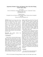
Figure 2: The
survey merges two
interleaved strips

(a night’s observa-
tion) into a stripe.
The stripe is proc-
essed by the pipe-
line to produce the
photo objects.
comes public. In addition, the SkyServer will get better documentation and tools as we gain more experi-
ence with how it is used.
Database Logical Design
The SDSS processing pipeline at Fermi Lab examines the images from the telescope’s 5 color bands and
identifies objects as a star, a galaxy, or other (trail, cosmic ray, satellite, defect). The classification is
probabilistic—it is sometimes difficult to distinguish a faint star from a faint galaxy. In addition to the
basic classification, the pipeline extracts about 400 object attributes, including a 5-color atlas cutout image
of the object (the raw pixels).

The actual observations are taken in stripes that are about 2.5º wide and 130º long. The stripes are proc-
essed one field at a time (a field has 5 color frames as in figure 2.) Each field in turn contains many ob-
jects. These stripes are in fact the mosaic of two night’s observation (two strips) with about 10% overlap
between the observations. Also, the stripes themselves have some overlaps near the horizon. Conse-
quently, about 10% of the objects appear more than once in the pipeline. The pipeline picks one object
instance as primary but all instances are recorded in the database. Even more challenging, one star or gal-
axy often overlaps another, or a star
is part of a cluster. In these cases
child objects are deblended from the
parent object, and each child also
appears in the database (deblended
parents are never primary.) In the
end about 80% of the objects are
primary.

The photo objects have positional
attributes (right ascension,
declination, (x,y,z) in the J2000
coordinate system, and HTM index).
Objects have the five magnitudes and five error bars in five color bands measured in six different ways.
Galactic extents are measured in several ways in each of the 5 color bands with error estimates (Petrosian,
Stokes, DeVaucouleurs, and ellipticity metrics.) The pipeline assigns a few hundred properties to each ob-
ject – these attributes are variously called flags, status, and type. In addition to their attributes, objects
have a profile array, giving the luminance in concentric rings around the object.


The photo object attributes are represented in the SQL database in several ways. SQL lacks arrays or other
constructors. So rather than representing the 5 color magnitudes as an array, they are represented as scalars
indexed by their names ModelMag_r is the name of the “red” magnitude as measured by the best model
fit to the data. In other cases, the use of names was less natural (for example in the profile array) and so the
data is encapsulated by access functions that extract the array elements from a blob holding the array and
its descriptor – for example array(profile,3,5) returns profile[3,5]. Spectrograms are measured for
approximately 1% of the objects. Most objects have estimated (rather than measured) redshifts recorded in
the photoZ table. To speed spatial queries, a neighbors table is computed after the data is loaded. For
every object the neighbors table contains a list of all other objects within ½ arcminute of the object (typi-
cally 10 objects). The pipeline also tries to correlate photo object with objects in other catalogs: United
States Naval Observatory [USNO], Röntgen Satellite [ROSAT], Faint Images of the Radio Sky at Twenty-
centimeters [FIRST], and others. These correlations are recorded in a set of relationship tables.

The result is a star-schema (see Figure 3) with the photoObj table in the center and fields, frames, photoZ,
neighbors, and connections to other surveys clustered about it. The 14 million photoObj records each have
about 400 attributes describing the object – about 2KB per record. The frame table describes the process-
ing for a particular color band of a field. Not shown in Figure 3 is the metadata DataConstants table that
holds the names, values, and documentation for all the photoObj flags. It allows us to use names rather
than binary values (e.g. flags & fPhotoFlags(‘primary’)).

4



Spectrograms are the second kind of object. About 600 spectra are observed at once using a single plate – a
metal disk drilled with 600 carefully placed holes, each holding an optical fiber going to a different CCD
spectogram. The plate description is stored in the plate table, and the description of the spectrogram and
its GIF are stored in the specObj table. The pipeline processing extracts about 30 spectral lines from each
spectrogram. The spectral lines are stored in the SpecLine table. The SpecLineIndex table has derived line
attributes used by astronomers to characterize the types and ages of astronomical objects. Each line is
cross-correlated with a model and corrected for redshift. The resulting line attributes are stored in the
xcRedShift table. Lines characterized as emission lines (about one per spectrogram) are described in the
elRedShift table.

There is also a set of tables used to monitor the data loading process and to support the web interface. Per-
haps the most interesting are the Tables, Columns, DataConstants, and Functions tables. The SkyServer
database schema is documented (in html) as comments in the schema text. We wrote a parser that converts
this schema to a collection of tables. Part of the sky server website lets users explore this schema. Having
the documentation imbedded in the schema makes maintenance easier and assures that the documentation
is consistent with reality ( The comments are also pre-
sented in tool tips by the Query Tool we built
Figure 3: The photoObj table at left is the center of one star schema describing photographic objects.
The SpecObj table at right is the center of a star schema describing spectrograms and the extracted spec-
tral lines. The photoObj and specObj tables are joined by objectId. Not shown are the dataConstants
table that names the photoObj flags and tables that support web access and data loading.

5

Database Access Design – Views, Indices, and Access Functions
The photoObj table contains many types of objects (primaries, secondaries, stars, galaxies,…). In some
cases, users want to see all the objects, but typically, users are just interested in primary objects (best in-
stance of a deblended child), or they want to focus on just Stars, or just Galaxies. Several views are de-
fined on the PhotoObj table to facilitate this subset access:
PhotoPrimary: photoObj records with flags(‘primary’)=true
PhotoSecondary: photoObj records with flags(‘secondary’)=true
PhotoFamily: photoObj that is not primary or secondary.
Sky: blank sky photoObj recods (for calibration).
Unknown: photoObj records of type “unknown”
Star: PrimaryObjects subsetted with type=’star’
Galaxy: PrimaryObjects subsetted with type=’galaxy’
SpecObj: Primary SpecObjAll (dups and errors removed)

Most users will work in terms of these views rather than
the base table. In fact, most of the queries are cast in terms
of these views. The SQL query optimizer rewrites such
queries so that they map down to the base photoObj table
with the additional qualifiers.

To speed access, the base tables are heavily indexed (these
indices also benefit view access). In a previous design
based on an object-oriented database ObjectivityDB™
[Thakar], the architects replicated vertical data slices in tag
tables that contain the most frequently accessed object at-
tributes. These tag tables are about ten times smaller than the base tables (100 bytes rather than 1,000
bytes) – so a disk-oriented query runs 10x faster if the query can be answered by data in the tag table.

Our concern with the tag table design is that users must know which attributes are in a tag table and must
know if their query is “covered” by the fields in the tag table. Indices are an attractive alternative to tag

tables. An index on fields A, B, and C gives an automatically managed tag table on those 3 attributes plus
the primary key – and the SQL query optimizer automatically uses that index if the query is covered by
(contains) only those 3 fields. So, indices perform the role of tag tables and lower the intellectual load on
the user. In addition to giving a column subset, thereby speeding access by 10x to 100x. Indices can also
cluster data so that searches are limited to just one part of the object space. The clustering can be by type
(star, galaxy), or space, or magnitude, or any other attribute. Microsoft’s SQL Server limits indices to 16
columns – that constrained our design choices.

Today, the SkyServer database has tens of indices, and more will be added as needed. The nice thing about
indices is that when they are added, they speed up any queries that can use them. The downside is that they
slow down the data insert process – but so far that has not been a problem. About 30% of the SkyServer
storage space is devoted to indices.

In addition to the indices, the database design includes a fairly complete set of foreign key declarations to
insure that every profile has an object; every object is within a valid field, and so on. We also insist that all
fields are non-null. These integrity constraints are invaluable tools in detecting errors during loading and
they aid tools that automatically navigate the database. You can explore the database design using web in-
terface at
Figure 4. Count of records and bytes
in major tables. Indices add 50% more
space.
Table Records Bytes
Field 14k

60MB

Frame 73k

6GB

PhotoObj 14m

31GB

Profile 14m

9GB

Neighbors 111m

5GB

Plate 98

80KB

SpecObj 63k

1GB

SpecLine 1.7m

225MB

SpecLineIndex 1.8m

142MB

xcRedShift 1.9m

157MB

elRedShift 51k

3MB



6


Spatial Data Access
The SDSS scientists are especially interested in the galactic clustering and large-scale structure of the uni-
verse. In addition, the visual interface routinely asks for all objects in a certain
rectangular or circular area of the celestial sphere. The SkyServer uses three different coordinate systems.
First right-ascension and declination (comparable to latitude-longitude in celestial coordinates) are ubiqui-
tous in astronomy. To make arc-angle computations fast, the (x,y,z) unit vector in J2000 coordinates is
stored. The dot product or the Cartesian difference of two vectors
are quick ways to determine the arc-angle or distance between them.

To make spatial area queries run quickly, we integrated the Johns
Hopkins hierarchical triangular mesh (HTM) code [HTM, Kunszt]
with SQL Server. Briefly, HTM inscribes the celestial sphere
within an octahedron and projects each celestial point onto the sur-
face of the octahedron. This projection is approximately iso-area.
The 8 octahedron triangular faces are each recursively decomposed
into 4 sub-triangles. SDSS uses a 20-deep HTM so that the indi-
vidual triangles are less than .1 square arcsecond.

The HTM ID for a point very near the north pole (in galactic coor-

dinates) would be something like 2,3,,3 (see Figure 5). These HTM IDs are encoded as 64-bit strings
(bigints). Importantly, all the HTM IDs within the triangle 6,1,2,2 have HTM IDs that are between 6,1,2,2
and 6,1,2,3. When the HTM IDs are stored in a B-tree index, simple range queries provide quick index for
all the objects within a given triangle.

The HTM library is an external stored procedure wrapped in a table-valued stored procedure
spHTM_Cover(<area>). The <area> can be either a circle (ra, dec, radius), a half-space (the intersection of
planes), or a polygon defined by a sequence of points. A typical area might be ‘CIRCLE J2000, 30.1, -10.2 .8’
which defines an 0.8 arc minute circle around the (ra,dec) = (30.1, -10.2)
2
. The spHTM_Cover table val-
ued function has the following template:
CREATE FUNCTION spHTM_Cover (@Area VARCHAR(8000)) the area to cover
RETURNS @Triangles TABLE ( returns table
HTMIDstart BIGINT NOT NULL PRIMARY KEY, start of triangle
HTMIDend BIGINT NOT NULL) end of triangle

The procedure call: select * from spHTM_Cover(‘Circle J2000 12 5.5 60.2 1’) returns the following
table with four rows, each row defining the start and end of a 12-deep HTM triangle.
HTMIDstart HTMIDend
3,3,2,0,0,1,0,0,1,3,2,2,2,0 3,3,2,0,0,1,0,0,1,3,2,2,2,1
3,3,2,0,0,1,0,0,1,3,2,2,2,2 3,3,2,0,0,1,0,0,1,3,2,2,3,0
3,3,2,0,0,1,0,0,1,3,2,3,0,0 3,3,2,0,0,1,0,0,1,3,2,3,1,0
3,3,2,0,0,1,0,0,1,3,2,3,3,1 3,3,2,0,0,1,0,0,1,3,3,0,0,0
One can join this table with the photoObj or specObj tables to get spatial subsets. There are many exa m-
ples of this in the sample queries below (see Q1 for example).

The spHTM_Cover() function is a little too primitive for most users, they actually want the objects nearby a
certain object, or they want all the objects in a certain area – and they do not want to have to pick the HTM
depth. So, the following family of functions is supported:

fGet{Nearest | Nearby} {Obj | Frame | Mosaic} Eq (ra, dec, radius_arc_minutes)
fGet{Nearest | Nearby} {Obj | Frame | Mosaic} XYZ (x, y, z, radius_arc_minutes)

2
The full syntax for areas is:
CIRCLE J2000 depth ra dec radius_arc_minutes
CIRCLE CARTESIAN depth x y z radius_arc_minutes
CONVEX J2000 depth n ra1 dec1 ra2 dec2 … ran decn // a polygon
CONVEX CARTESIAN x1 y1 z1 x2 y2 z2… xn yn zn // a polygon
DOMAIN depth k n1 x1 y1 z1 d1 x2 y2 z2 d2… xn1 yn1 zn1 dn1
n2 x1 y1 z1 d1 x2 y2 z2 d2… xn2 yn2 zn2 dn2

nk x1 y1 z1 d1 x2 y2 z2 d2… xnk ynk znk dnk

2
2,2
2,1
2,0
2,3
2,3,0
2,3,1
2,3,2 2,3,3
2
2,2
2,1
2,0
2,32,2
2,1
2,0
2,3

2,3,0
2,3,1
2,3,2 2,3,3
2,3,0
2,3,1
2,3,2 2,3,3
Figure 5: A Hierarchical Triangular
Mesh (HTM) recursively assigns a
number to each point on the sphere.
Most spatial queries use the HTM
index to limit searches to a small set
of triangles.

7


For example: fGetNeaestObjEq(1,1,1) returns the nearest object coordinates within one arcminute of
equatorial coordinate (1º, 1º). These procedures are frequently used in the 20 queries and in the website
access pages.

In summary, the logical database design consists of photographic and spectrographic objects. They are
organized into a pair of snowflake schema. Subsetting views and many indices give convenient access to
the conventional subsets (stars, galaxies, ). Several procedures are defined to make spatial lookups con-
venient. documents these functions in more detail.
Database Physical Design and Performance
The SkyServer initially took a simple approach to database design – and since that worked, we stopped
there. The design counts on the SQL Server data storage engine and query optimizer to make all the intel-
ligent decisions about data layout and data access.

The data tables are all created in one file group. The file group consists of files spread across all the disks.

If there is only one disk, this means that all the data (about 80 GB) is on one disk, but more typically there
are 4 or 8 disks. Each of the N disks holds a file that starts out as size 80 GB/N and automatically grows as
needed. SQL Server stripes all the tables across all these files and hence across all these disks. When read-
ing or writing, this automatically gives the sum of the disk bandwidths without any special user program-
ming. SQL Server detects the sequential access, creates the parallel prefetch threads, and uses multiple
processors to analyze the data as quickly as the disks can produce it. Using commodity low-end servers we
measure read rates of 150 MBps to 450 MBps depending on how the disks are configured.

Beyond this file group striping; SkyServer uses all the SQL Server default values. There is no special tun-
ing. This is the hallmark of SQL Server – the system aims to have “no knobs” so that the out-of-the box
performance is quite good. The SkyServer is a testimonial to that goal.

So, how well does this work? The appendix gives detailed timings on the twenty queries; but, to summa-
rize, a typical index lookup runs primarily in memory and completes within a second or two. SQL Server
expands the database buffer pool to cache frequently used data in the available memory. Index scans of
the 14M row photo table run in 7 seconds “warm” (2 m records per second when CPU-bound), and 18 sec-
onds cold (100 MBps when disk bound), on a 4-disk 2-CPU Server. Queries that scan the entire 30 GB
photoObj table run at about 150MBps and so take about 3 minutes. These scans use the available CPUs
and disks to run in parallel. In general we see 4-disk workstation-class machines running at the 150 MBps,
while 8-disk server-class machines can run at 300 MBps.

When the SkyServer project began, the existing software (ObjectivityDB™ on Linux or Windows) was
delivering 0.5 MBps and heavy CPU consumption. That performance has now improved to 300 MBps and
about 20 instructions per byte (measured at the SQL level). This gives 5-second response to simple que-
ries, and 5-minute response to full database scans. The SkyServer goal was 50MBps at the user level on a
single machine. As it stands SQL Server and the Compaq hardware exceeded these performance goals by
500% so we are very pleased with the design. As the SDSS data grows, arrays of more powerful ma-
chines should allow the SkyServer to return most answers within seconds or minutes depending on whether
it is an index search, or a full-database scan.
Database Load Process

The SkyServer is a data warehouse: new data is added in batches, but mostly the data is queried. Of
course these queries create intermediate results and may deposit their answers in temporary tables, but the
vast bulk of the data is read-only.

Occasionally, a brand new schema must be loaded, so the disks were chosen to be large enough to hold
three complete copies of the database (70GB disks).

From the SkyServer administrator’s perspective, the main task is data loading which includes data vali-
dation. When new photo objects or spectrograms come out of the pipeline, they must be added to the da-

8


tabase quickly. We are the system administrators – so we wanted this loading process to be as automatic as
possible.

The Beowulf data pipeline produces FITS files [FITS]. A filter program converts this output to produce
column-separated values (CSV) files, and PNG files [SDSS-EDR]. These files are then copied to the
SkyServer. From there, a script-level utility we wrote loads the data using the SQL Server’s Data Trans-
formation Service (DTS). DTS does both data conversion and the integrity checks. It also recognizes file
names in some fields, and uses the name to insert the image file (PNG or JPEG) as a blob field of the re-
cord. There is a DTS script for each table load step. In addition to loading the data, these DTS scripts
write records in a loadEvents table recording the time of the load, the number of records in the source file
and the number of inserted records. The DTS steps also write trace files indicating the success or errors in
the load step. A particular load step may fail because the data violates foreign key constraints, or because
the data is invalid (violates integrity constraints.) A web user interface displays the load-events table and
makes it easy to examine the CSV file and the load trace file. The operator can (1) undo the load step, (2)
diagnose and fix the data problem, and (3) re-execute the load on the corrected data. If the input file is eas-
ily repaired, that is done by the administrator, but often the data needs to be regenerated. In either case the
first step is to UNDO the failed load step. Hence, the web interface has an UNDO button for each step.

The UNDO function works as follows. Each table in the database has an additional timestamp field that
records when the record was inserted (the field has Current_Timestamp as its default value.) The load
event record records the table name and the start and stop time of the load step. Undo consists of deleting
all records from the target table with an insert time between that start and stop time.

Loading runs at about 5 GB per hour (data conversion is very CPU intensive), so the current SkyServer
loads in about 12 hours. More than ½ this time goes into building or maintaining the indices.


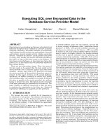
Figure 6: A screen shot of the SkyServer Data-
base operations interface. The SkyServer is oper-
ated via the Internet using Windows™ Terminal
Server, a remote desktop facility built into the
operating system. Both loading and software
maintenance are done in this way. This screen
shot shows a window into the backend system
after a load step has completed. It shows the
loader utility, the load monitor, a performance
monitor window and a database query window.
This remote operation has proved a godsend, al-
lowing the Johns Hopkins, Microsoft, and Fermi
Lab participants to perform operations tasks from
their offices, homes, or hotel rooms.

Personal SkyServer
A 1% subset of the SkyServer database (about 1/2 GB) that can fit on a CD or downloaded over the web
( This includes the web site and all
the photo and spectrographic objects in a 6º square of the sky. This personal SkyServer fits on laptops and
desktops. It is useful for experimenting with queries, for developing the web site, and for giving demos.

We also believe SkyServer will be great for education teaching both how to build a web site and how to
do computational science. Essentially, any classroom can have a mini-SkyServer per student. With disk
technology improvements, a large slice of the public data will fit on a single disk by 2003.
Hardware Design and Raw Performance
The SkyServer database is about 80 GB. It can run on a single processor system with just one disk, but the
production SkyServer runs on more capable hardware generously donated by Compaq Computer Corpora-
tion. Figure 7 shows the hardware configuration.

9



Figure 7: The SkyServer hardware configuration.
The web front-end is a dual processor running IIS
on a Compaq DL380. The Backend is SQL Server
running on a Compaq ML530 with ten UltraI160
SCSI disk drives. The machines communicate via
100Mbit/s Ethernet. The web server is connected to
the Fermilab Internet interface.

The web server runs Windows2000 on a Compaq ProLiant DL380 with dual 1GHz Pentium III processors.
It has 1GB of 133MHz SDRAM, and two mirrored Compaq 37GB 10K rpm Ultra160 SCSI disks attached
to a Compaq 64-Bit/66MHz Single Channel Ultra3 SCSI Adapter. This web server does almost no disk IO
during normal operation, but we clocked the disk subsystem at over 30MB/s. The web server is also a
firewall, it does not do routing and so acts as a firewall. It has a separate “private” 100Mbit/s Ethernet link
to the backend database server.

Most data mining queries are IO-bound, so the database server is configured to give fast sequential disk
bandwidth. It also helps to have healthy CPU power and high availability. The database server is a Compaq
ProLiant ML530 running SQL Server 2000 and Windows2000. It has two 1GHz Pentium III Xeon proces-

sors, 2GB of 133MHz SDRAM, a 2-slot 64bit/66MHz PCI bus, a 5-slot 64bit/33MHz PCI bus, and a 32bit
PCI bus with a single expansion slot. It has 12 drive bays for low-profile (1 inch) hot-pluggable SCA-2
SCSI drives, split into two SCSI channels of six disks each. It has an onboard dual-channel ultra2 LVD
SCSI controller, but we wanted greater disk bandwidth, so we added two Compaq 64-Bit/66MHz Single
Channel Ultra3 SCSI Adapters to the 64bit/66MHz PCI bus, and left the onboard ultra2 SCSI controller
disconnected. These Compaq ultra160 SCSI adapters are Adaptec 29160 cards with a Compaq BIOS.

The DL380 and the ML530 also have a complement of high-availability hardware components: redundant
hot-swappable power supplies, redundant hot-swappable fans, and hot-swappable SCA-2 SCSI disks.

The production database server is configured with 10 Compaq 37GB 10K rpm Ultra160 SCSI disks, five on
each SCSI channel. We use Windows 2000’s native software RAID to manage the disks as five mirrors
(RAID1’s), with each mirror split across the two SCSI channels. One mirrored volume is for the operating
system and software, and the remaining four volumes are for database files. The database file groups (data,
temp, and log) are spread across these four mirrors. SQL Server stripes the data across the four volumes,
effectively managing the data disks as a RAID10 (striping plus mirroring). This configuration can scan data
at 140 MB/s for a simple query like:
select count(*)
from photoObj
where (r-g)>1.

Before the production database server was deployed, we ran some tests to find the maximum IO speed for
database queries on our ML530 system. We’re quite happy with the 140 MB/s performance of the conser-
vative, reliable production server configuration on the 60GB public EDR (Early Data Release) data. How-
ever, we’re about to implement an internal SkyServer which will contain about 10 times more data than
the public SkyServer: about 500-600GB. For this server, we’ll probably need more raw speed.

For the max-speed tests, we used our ML530 system, plus some extra devices that we had on-hand: an as-
sortment of additional 10K rpm ultra160 SCSI disks, a few extra Adaptec 29160 ultra160 SCSI controllers,
and an external eight-bay two-channel ultra160 SCSI disk enclosure. We started by trying to find the per-

formance limits of each IO component: the disks, the ultra160 SCSI controllers, the PCI busses, and the
memory bus. Once we had a good feel for the IO bottlenecks, we added disks and controllers to test the
system’s peak performance.

For each test setup, we created a stripe set (RAID0) using Windows 2000’s built-in software RAID, and ran
two simple tests. First, we used the MemSpeed utility (v2.0 [MemSpeed]) to test raw sequential IO speed
using 16-deep unbuffered IOs. MemSpeed issues the IO calls and does no processing on the results, so it
gives an idealized, best-case metric. In addition to the unbuffered IO speed, MemSpeed also does several

Compaq D1380
2x1Ghz PIII

Win2k, IIS5

Compaq M1530

2x1Ghz PIII
2GB ram

10x 10krpm SCSI160
drives
On 66/64 U160 ctlr

Win2k, SQL2k


10


tests on the system’s memory and memory bus. It tests memory read, write, and memcpy rates - both sin-

gle-threaded, and multi-threaded with a thread per system CPU. These memory bandwidth measures sug-
gest the system’s maximum IO speed. After running MemSpeed tests, we copied a sample 4GB un-indexed
SQL Server database onto the test stripe set and ran a very simple select count(*) query to see how
SQL Server’s performance differed from MemSpeed’s idealized results.

Figure 8 shows our performance results.
• Individual disks: The tests used three different disk models: the Compaq 10K rpm 37GB disks in the
ML530, some Quantum 10K rpm 18GB disks, and a 37GB 10K rpm Seagate disk. The Compaq disks
could perform sequential reads at 39.8 MB/s, the old Quantums were the slowest at 37.7 MB/s, and the
new Seagate churned out 51.7 MB/s! The “linear quantum” plot on Figure 8 shows the best-case
RAID0 performance based on a linear scaleup of our slowest disks.
• Ultra160 SCSI: A single ultra160 SCSI channel saturates at about 123 MB/s. It makes no sense to
add more than three of disks to a single channel. Ultra160 delivers 77% of its peak advertised 160
MB/s.
• 64bit/33MHz PCI: With three ultra160 controllers attached to the 64bit/33MHz PCI bus, the bus satu-
rates at about 213 MB/s (80% of its max. burst speed of 267 MB/s). This is not quite enough band-
width to handle the traffic from six disks.
• 64bit/66MHz PCI: We didn’t have enough disks, controllers, or 64bit/66MHz expansion slots to test
the bus’s 533 MB/s peak advertised performance.
• Memory bus: MemSpeed reported single-threaded read, write, and copy speeds of 590 MB/s, 274
MB/s, and 232 MB/s respectively, and multithreaded read, write, and copy speeds of 849 MB/s, 374
MB/s, and 300 MB/s respectively.

MBps vs Disk Config
0
50
100
150
200
250

300
350
400
450
500
1disk 2disk 3disk 4disk 5disk 6disk 7disk 8disk 9disk 10disk 11disk 12disk 12disk
2vol
MBps
memspeed avg.
mssql
linear quantum
64bit/33MHz pci bus
1 disk controler saturates
1 PCI bus saturates
SQL saturates CPU
added 2nd ctlr
added 4th ctlr

Figure 8: Sequential IO speed is important
for data mining queries. This graph shows
the sequential scan speed (megabytes per
second) as more disks and controllers are
added (one controller added for each 3
disks). It indicates that the SQL IO system
can process about 320MB/s (and 2.7 million
records per second) before it saturates.

After the basic component tests, the system was configured to avoid SCSI and PCI bottlenecks. Initially
three ultra160 channels were configured: two controllers connected to the 64bit/66MHz PCI bus, and one
connected to the 64bit/33MHz bus. Disks were added to the controllers one-by-one, never using more than

three disks on a single ultra160 controller. Surprisingly, both the simple MemSpeed tests and the SQL
Server tests scaled up linearly almost perfectly to nine disks. The ideal disk speed at nine disks would be
339 MB/s, and we observed 326.7 MB/s from MemSpeed, and 322.4 MB/s from SQL Server. To reach the
performance ceiling yet, a fourth ultra160 controller (to the 64bit/33MHz PCI bus) was added along with
more disks. The MemSpeed results continued to scale linearly through 11 disks. The 12-disk MemSpeed
result fell a bit short of linear at 433.8 MB/s (linear would have been 452 MB/s), but this is probably be-
cause we were slightly overloading our 64bit/33MHz PCI bus on the 12-disk test. SQL Server read speed
leveled off at 10 disks, remaining in the 322 MB/s ballpark. Interestingly, SQL Server never fully saturated
the CPU’s for our simple tests. Even at 322 MB/s, CPU utilization was about 85%. Perhaps the memory
was saturated at this point. 322 MB/s is in the same neighborhood as the memory write and copy speed
limits that we measured with MemSpeed.


11


Figure 9 shows the relative IO density of the queries. It shows that the queries issue about a thousand IOs
per CPU second. Most of these IOs are 64KB sequential reads of the indices or the base data. So, each
CPU generates about 64MB of IO per second. Since these CPUs each execute about a billion instructions
per second, that translates to an IO density of a million instructions per IO and about 16 instructions per
byte of IO – both these numbers are an order of magnitude higher than Amdahl’s rules of thumb. Using
SQLserver a CPU can consume about five million records per second if the data is in main memory.

cpu vs IO
1E+0
1E+1
1E+2
1E+3
1E+4
1E+5

1E+6
1E+7
0.01 0.1 1. 10. 100. 1,000.CPU sec
IO count
1,000 IOs/cpu sec
~1,000 IO/cpu sec
~ 64 MB IO/cpu sec

Figure 9: A measurement of the relative IO and
CPU density of each query. This load generates
1,000 IOs per CPU second and generates 64 MB of
IO per CPU second.



12


1
10
100
1000
8 1 9 10A 10 19 12 16 4 2 13 11 6 7 15B 17 14 15A 5 3 20 18
seconds
cpu time
elapsed time

Figure 10: Summary of the query execution times (on a dual processor system). The system is disk
limited where the CPU time is less than 2x the elapsed time (e.g., in all cases). So 2x more disks would
cut the time nearly in half. The detailed statistics are in the table in the Appendix.

A Summary of the Experience Implementing the Twenty Queries
The Appendix has each of the 20 queries along with a description of the query plans and measurements of
the CPU time, elapsed time, and IO demand. This section just summarizes the appendix with general
comments.

First, all the 20 queries have fairly simple SQL equivalents. This was not obvious when we started and
we were very pleased to find it was true. Often the query can be expressed as a single SQL statement. In
some cases, the query is iterative, the results of one query feeds into the next. These queries correspond to
typical tasks astronomers would do with a TCL script driving a C++ program, extracting data from the ar-
chive, and then analyzing it. Traditionally most of these queries would have taken a few days to write in
C++ and then a few hours or days to run against the binary files. So, being able to do the query simply and
quickly is a real productivity gain for the Astronomy community.

Many of the queries run in a few seconds. Some that involve a sequential scan of the database take about 3
minutes. One involves a spatial join and takes ten minutes. As the data grows from 60GB to 1TB, the
queries will slow down by a factor of 20. Moore’s law will probably give 3x in that time, but still, things
will be 7x slower. So, future SkySevers will need more than 2 processors and more than 4 disks. By using
CPU and disk parallelism, it should be possible to keep response times in the “few minutes” range.

The spatial data queries are both simple to state and quick to execute using the HTM index. We circum-
vented a limitation in SQL Server by pre-computing the neighbors of each object. Even without being
forced to do it, we would have created this materialized view to speed queries. In general, the queries bene-
fited from indices on the popular fields.

In looking at the queries in the Appendix, it is not obvious how they were constructed – they are the fin-
ished product. In fact, they were constructed incrementally. First we explored the data a bit to see the
rough statistics – either counting (select count(*) from…) or selecting the first 10 answers (select top
10 a,b,c from ). These component queries were then composed to form the final query shown in the
Appendix.

It takes both a good understanding of astronomy, a good understanding of SQL, and a good understanding
of the database to translate the queries into SQL. In watching how “normal” astronomers access the SX
web site, it is clear that they use very simple SQL queries. It appears that they use SQL to extract a subset
of the data and then analyze that data on their own system using their own tools. SQL, especially complex
SQL involving joins and spatial queries, is just not part of the current astronomy toolkit.

Indeed, our actual query set includes 15 additional queries posed by astronomers using the Objectivity™
archive at ( Those 15 queries are much simpler and run more
quickly than most of the original 20 queries.

A good visual query tool that makes it easier to compose SQL would ameliorate part of this problem, but
this stands as a barrier to wider use of the SkyServer by the astronomy community. Once the data is pro-

13


duced, there is still a need to understand it. We have not made any progress on the problem of data visuali-
zation.

It is interesting to close with two anecdotes about the use of the SkyServer for data mining. First, when it
was realized that query 15 (find asteroids) had a trivial solution, one colleague challenged us to find the
“fast moving” asteroids (the pipeline detects slow-moving asteroids). These were objects moving so fast,
that their detections in the different colors were registered as entirely separate objects (the 5 colors are ob-
served at 5 different 1-minute intervals as the telescope image drifts across the sky – this time-lapse causes
slow-moving images to appear as 5 dots of different colors while fast moving images appear as 5 streaks.)
This was an excellent test case – our colleague had written a 12 page tcl script that had run for 3 days on
the dataset consisting of binary FITS tables. So we had a benchmark to work against. It took a long day to
debug our understanding of the data and to develop a query (see query 15A). The resulting query runs in
about 10 minutes and finds 3 objects. If we create a supporting index (takes about 10 minutes) then the
query runs in less than a minute. Indeed, we have found other fast-moving objects by experimenting with

the query parameters. Being able to pose questions in a few hours and get answers in a few minutes
changes the way one views the data: you can experiment with it almost interactively. When queries take 3
days and hundreds of lines of code, one asks questions cautiously.

A second story relates to the fact that 99% of the object’s spectra will not be measured and so their red-
shifts will not be measured. As it turns out, the objects’ redshifts can be estimated by their 5-color optical
measurements. These estimates are surprisingly good [Budavari1, Budavari2]. However, the estimator
requires a training set. There was a part of parameter space – where only 3 galaxies were in the training
data and so the estimator did a poor job. To improve the estimator, we wanted to measure the spectra of
1,000 such galaxies. Doing that required designing some plates that measure the spectrograms. The plate
drilling program is huge and not designed for this task. We were afraid to touch it. But, by writing some
SQL and playing with the data, we were able to develop a drilling plan in an evening. Over the ensuing 2
months the plates were drilled, used for observation, and the data was reduced. Within an hour of getting
the data, they were loaded into the SkyServer database and we have used them to improve the redshift pre-
dictor — it became much more accurate on that class of galaxies. Now others are asking our help to de-
sign specialized plates for their projects.

We believe these two experiences and many similar ones, along with the 20+15 queries in the appendix, are
a very promising sign that commercial database tools can indeed help scientists organize their data for data
mining and easy access.
Acknowledgements
We acknowledge our obvious debt to the people who built the SDSS telescope, those who operate it, those
who built the SDSS processing pipelines, and those who operate the Fermilab pipeline. The SkyServer
data depends on the efforts of all those people. In addition Robert Lupton has been very helpful in explain-
ing the photo-object processing and some of the subtle meanings of the attributes, Mark Subbarao has been
equally helpful in explaining the spectrogram attributes and Steve Kent has helped us to understand the
observations better. James Annis, Xiaohui Fan, Gordon Richards, Michael Strauss, and Paula Szkody
helped us compose some of the more complex queries. David DeWitt helped us improve the presentation.
We thank Compaq and Microsoft for donating the project’s hardware and software.

14


References
[Barclay] T. Barclay, D.R. Slutz, J. Gray, “TerraServer: A Spatial Data Warehouse,” Proc. ACM SIGMOD
2000, pp: 307-318, June 2000
[Budavari1] T. Budavari, et al., “Creating Spectral Templates from Multicolor Redshift Surveys,” AJ 120
(2000).
[Budavari2] T. Budavari, et al., “Photometric Redshifts from Reconstructed Quasar Templates,” AJ 122
(2001) 1163-1171.
[FIRST] Faint Images of the Radio Sky at Twenty-centimeters (FIRST)
[FITS] Flexible Image Transport System (FITS),
[HTM] Hierarchical Triangular Mesh,
[Kunszt] P. Z. Kunszt, A. S. Szalay, I. Csabai, A. R. Thakar “The Indexing of the SDSS Science Archive”
ASP V. 216, Astronomical Data Analysis Software and Systems IX, eds. N. Manset, C. Veillet, D. Crab-
tree, San Francisco: ASP, pp. 141-145 (2000).
[Thakar] Thakar, A., Kunszt, P.Z., Szalay, A.S. and G.P. Szokoly: “Multi-threaded Query Agent and En-
gine for a Very Large Astronomical Database,” in Proc ADASS IX, eds. N. Manset, C. Veillet, D. Crab-
tree, (ASP Conference series), 216, 231 (2000).
[MAST] Multi Mission Archive at Space Telescope. :8080/index.html
[NED] NASA/IPAC Extragalactic Database,
[ROSAT] Röntgen Satellite (ROSAT)
[SDSS-EDR] C. Stoughton et. al. “The Sloan Digital Sky Survey Early Data Release,” The Astronomical
Journal, 123 1:485-548 (2002)
[SDSS-overview] D.G. York et. al. “The Sloan Digital Sky Survey: Technical Summary,” AJ V120, 1579,
also see also
[SDSS] D.G. York, et al., “The Sloan Digital Sky Survey: Technical Summary,” AJ 120 (2000) 1579-
1587,
[Simbad] SIMBAD Astronomical Database,
[Szalay1] A. Szalay, P. Z. Kunszt, A. Thakar, J. Gray, D. R. Slutz. “Designing and Mining Multi-Terabyte

Astronomy Archives: The Sloan Digital Sky Survey,” Proc. ACM SIGMOD 2000, pp. 451-462, June
2000
[Szalay2] A. Szalay, J. Gray, P. Z. Kunszt, T. Malik, A. Thakar, J. Raddick, C. Stoughton, J. vandenBerg,
“The SDSS SkyServer – Public Access to the Sloan Digital Sky Server Data,” Proc. ACM SIGMOD
2002, June 2002
[USNO] United States Naval Observatory
[Virtual Sky] Virtual Sky,
[VIzieR] VizieR Service,


15


Appendix: A Detailed Narrative of the Twenty Queries
This section presents each query, its translation to SQL, and a discussion of how the Query performs on the
SkyServer at Fermi Lab. The computer is a Compaq ProLiant Ml530 with two 1GHz Pentium III Xeon
processors, 2GB of 133MHz SDRAM; a 64bit/66MHz PCI bus with eight 10K rpm SCSI disks configured
as 4 mirrored volumes. The database, log, and temporary database, and logs are all spread across these
disks.

Some queries first define constants (see for example query 1) that are later used in the query – rather than
calling the constant function within the query. If we do not do this, the SQL query optimizer takes the very
conservative view that the function is not a constant and so the query plan calls the function for every tuple.
It also suspects that the function may have side effects, so the optimizer turns off parallelism. So, function
calls inside queries cause a 10x or more slowdown for the query and corresponding CPU cost increase. As
a workaround, we rarely use functions within a query – rather we define variables (e.g. @saturated in Q1)
and assign the function value to the variable before the query runs. Then the query uses these (constant)
variables.

Q1: Find all galaxies without saturated pixels within 1' of a given point.

The query uses the table valued function getNearbyObjEq() that does an HTM cover search to find
nearby objects. This handy function returns the object’s ID, distance, and a few other attributes. The query
also uses the Galaxy view to filter out everything but primary (good) galaxy objects.
declare @saturated bigint; initialized “saturated” flag
set @saturated = dbo.fPhotoFlags('saturated'); avoids SQL2K optimizer problem
select G.objID, GN.distance return Galaxy Object ID and
into ##results angular distance (arc minutes)
from Galaxy as G join Galaxies with
join fGetNearbyObjEq(185,-0.5, 1) as GN objects within 1’ of ra=185 & dec= 5
on G.objID = GN.objID connects G and GN
where (G.flags & @saturated) = 0 not saturated
order by distance sorted nearest first
The query returns 19 galaxies in 50 milliseconds of CPU time and 0.19 seconds of elapsed time. The
following picture shows the query plan (the rows from the table-valued function GetNerabyObjEQ() are
nested-loop joined with the photoObj table – each row from the function is used to probe the photoObj ta-
ble to test the saturated flag, the primary object flag, and the galaxy type.). The function returns 22 rows
that are joined with the photoObj table on the ObjID primary key to get the object’s flags. 19 of the ob-
jects are not saturated and are primary galaxies, so they are sorted by distance an inserted in the ##results
temporary table.

Q2: Find all galaxies with blue surface brightness between and 23 and 25 magnitude per square
arcseconds, and super galactic latitude (sgb) between (-10º, 10º), and declination less than zero.
The surface brightness is defined as the logarithm of flux per unit area on the sky. Since the magnitude is -
2.5 log(flux), the SB is –2.5 log(flux/R
2
π). The SkyServer pipeline precomputed the value rho = -5 log( R )
– 2.5 log (π), where R is the radius of the galaxy. Thus, for a constraint on the surface brightness in the g
band we can use the combination g+rho.

select objID Get the object identifier

into ##results
from Galaxy of all the galaxies that have
where ra between 170 and 190 designated ra/dec (need galactic coordinates)
and dec < 0 declination less than zero.
and g+rho between 23 and 25 g = blue magnitude,
rho= 5*ln(r)
g+rho = SB per sq arc sec is between 23 and 25

16


This query finds 191,062 objects in 18.6 seconds elapsed, 14 seconds of CPU time. This is a parallel scan
of the XYZ index of the PhotoObj table (Galaxy is a view of that table that only shows primary objects that
are of type Galaxy). The XYZ index covers this query (contains all the necessary fields). The query spends
2 seconds inserting the answers in the ##results set, if the query just counts the objects, it runs in 16 sec-
onds.


Q3: Find all galaxies brighter than magnitude 22, where the local extinction is >0.175.
The extinction indicates how much light is absorbed by that dust that is between the object and the earth.
There is an extinction table, giving the extinction for every “cell”, but the extinction is also stored as an
attribute of each element of the PhotoObj table, so the simple query is:
select objID find the object IDs
into ##results
from Galaxy join Galaxies with Extinction table
where r < 22 where brighter than 22 magnitude
and reddening_r> 0.175 extinction more than 0.175
The query returns 488,183 objects in 168 seconds and 512 seconds of CPU time – the large CPU time re-
flects an SQL feature affectionately known as the “bookmark bug”. SQL thinks that very few galaxies
have r<22, so it finds those in the index and then looks up each one to see if it has reddening_r > .175. We

could force it to just scan the base table (by giving it a hint), but that would be cheating. The query plan
does a sequential scan of the 14 million records in the PhotoObj.xyz index to find the approximately
500,000 galaxy objIDs that have magnitude less than 22. Then it does a lookup of each of these objects in
the base table (1/2 a million “bookmark” lookups) to check the reddening. The query uses about 30% of
one of the two CPUs – much of this is spent inserting the ½ million answer records. If the extinction ma-
trix were used, this query could use the HTM index and run about five times faster. The choice of a book-
mark lookup may be controversial, but it does run quickly.

Q4: Find galaxies with an isophotal surface brightness (SB) larger than 24 in the red band, with an
ellipticity>0.5, and with the major axis of the ellipse between 30” and 60”arc seconds (a large galaxy).
Each of the five color bands has been pre-processed into a bitmap image that is broken into 15 concentric
rings. The rings are further divided into octants. This information is stored in the object’s profile. The in-
tensity of the light in each ring and octant is pre-processed to compute surface brightness, ellipticity, major
axis, and other attributes. These derived attributes are stored with the PhotoObj, so the query operates on
these derived quantities.
select ObjID put the qualifying galaxies in a table
into ##results
from Galaxy select galaxies
where r + rho < 24 brighter than magnitude 24 in the red spectral band
and isoA_r between 30 and 60 major axis between 30" and 60"
and (power(q_r,2) + power(u_r,2)) > 0.25 square of ellipticity is > 0.5 squared.
The query returns 787 rows in 18 seconds elapsed, 9 seconds of CPU time. It does a parallel scan of the
NEO index on the photoObj Table that covers the object type, status, flags, and also isoA, q_r, and r. The
query then does a bookmark lookup on the qualifying galaxies to check the r+rho and q_r
2
+u_r
2
terms.
The resulting records are inserted in the answer set.

17



Q5: Find all galaxies with a deVaucouleours profile (r¼ falloff of intensity on disk) and the photo-
metric colors consistent with an elliptical galaxy. As discussed in Q4, the deVaucouleours profile in-
formation is precomputed from the concentric rings during the pipeline processing. There is a likelihood
value stored in the table, which tells whether the deVaucouleours profile or an exponential disk is a better
fit to the galaxy.
declare @binned bigint; initialized “binned” literal
set @binned = dbo.fPhotoFlags('BINNED1') + avoids SQL2K optimizer problem
dbo.fPhotoFlags('BINNED2') +
dbo.fPhotoFlags('BINNED4') ;
declare @blended bigint; initialized “blended” literal
set @blended = dbo.fPhotoFlags('BLENDED'); avoids SQL2K optimizer problem
declare @noDeBlend bigint; initialized “noDeBlend” literal
set @noDeBlend = dbo.fPhotoFlags('NODEBLEND'); avoids SQL2K optimizer problem
declare @child bigint; initialized “child” literal
set @child = dbo.fPhotoFlags('CHILD'); avoids SQL2K optimizer problem
declare @edge bigint; initialized “edge” literal
set @edge = dbo.fPhotoFlags('EDGE'); avoids SQL2K optimizer problem
declare @saturated bigint; initialized “saturated” literal
set @saturated = dbo.fPhotoFlags('SATURATED'); avoids SQL2K optimizer problem
select objID
into ##results
from Galaxy as G count galaxies
where lDev_r > 1.1 * lExp_r red DeVaucouleurs fit likelihood greater than disk fit
and lExp_r > 0 exponential disk fit likelihood in red band > 0
Color cut for an elliptical galaxy courtesy of James Annis of Fermilab

and (G.flags & @binned) > 0
and (G.flags & ( @blended + @noDeBlend + @child)) != @blended
and (G.flags & (@edge + @saturated)) = 0
and (G.petroMag_i > 17.5)
and (G.petroMag_r > 15.5 OR G.petroR50_r > 2)
and (G.petroMag_r < 30 and G.g < 30 and G.r < 30 and G.i < 30)
and ((G.petroMag_r-G.reddening_r) < 19.2)
and ( ( ((G.petroMag_r - G.reddening_r) < (13.1 + deRed_r < 13.1 +
(7/3)*(G.g - G.r) + 0.7 / 0.3 * deRed_gr
4 *(G.r - G.i) -4 * 0.18 )) 1.2 / 0.3 * deRed_ri
and (( G.r - G.i - (G.g - G.r)/4 - 0.18) BETWEEN -0.2 AND 0.2 )
)
or
( (( G.petroMag_r - G.reddening_r) < 19.5 ) deRed_r < 19.5 +
and (( G.r - G.i -(G.g - G.r)/4 18) > cperp = deRed_ri
(0.45 - 4*( G.g - G.r))) 0.45 - deRed_gr/0.25
and ((G.g - G.r) > ( 1.35 + 0.25 *(G.r - G.i)))
) )
The query found 40,005 objects in 166 seconds elapsed, 66 seconds of CPU time. This is parallel table
scan of PhotoObj table because there is no covering index. The fairly complex query evaluation all hides
in the parallel scan and parallel filter nodes at the right of the figure below.

Q6: Find galaxies that are blended with a star and output the deblended galaxy magnitudes.
Some objects overlap others. The most common cases are a star in front of a galaxy or a star in the halo of
another star. These “deblended” objects, record their “parent” objects in the database. So this query starts
with a deblended galaxy (one with a parent) and then looks for all stars that have the same parent. It then
outputs the five color magnitudes of the star and the parent galaxy.
select G.ObjID, G.u, G.g, G.r, G.i, G.z output galaxy and magnitudes.
into ##results
from galaxy G, star S for each galaxy

where G.parentID > 0 galaxy has a “parent”
and G.parentID = S.parentID star has the same parent
The query found 1,088,806 galaxy -star pairs in 41 seconds. Without an index on the parent attribute, this is a Car-
tesian product of two very large tables and would involve about 10
16
join steps. So, it makes good sense to
create an index or intermediate table that has the deblended stars. Fortunately, SkyServer already has a

18


parent index on the photoObj table, since we often want to find the children of a common parent. The
clause parentID>0 excludes galaxies with no parent. These two steps cut the task from about 10
20
down to
a near-linear 10
8
steps (because ½ the objects are galaxies and about 25% of them have parents). The
plan scans the Parent index and builds a hash table of parent IDs, galaxy IDs that have parents (about 3.7M
objects, so about 40MB). It then scans over the index a second time looking at stars that have parents. It
looks in the hash table to see if the parent is also a parent of a galaxy. If so, the galaxy ID and star ID are
inserted in the answer set.


Q7: Provide a list of star-like objects that are 1% rare.
The survey gets magnitude information about stars in 5 color bands. This query looks at the ratios of the
brightness in each band. (Luminosity ratios are magnitude differences because magnitudes are logarithms
of the actual brightness in that band). The query “bins” these magnitudes based on the 4-space of u-g, g-r,
r-i, i-z. Experimentation showed that dividing the bins in integer units worked well. We built a results
table that contains all the bins. The large-population bins are deleted, leaving only the rare ones (less than

500 members).
select cast(round((u-g),0) as int) as UG,
cast(round((g-r),0) as int) as GR,
cast(round((r-i),0) as int) as RI,
cast(round((i-z),0) as int) as IZ,
count(*) as pop
into ##results
from star
where (u+g+r+i+z) < 150 exclude bogus magnitudes (== 999)
group by cast(round((u-g),0) as int), cast(round((g-r),0) as int),
cast(round((r-i),0) as int), cast(round((i-z),0) as int)
order by count(*)

This query found 15,528 buckets in less than a minute. The first 140 buckets have 99% of the objects.
The query scans the UGRIZ index of the photoObj table in parallel to populate a hash table containing the
counts. When the scan is done, the hash table is sorted put into the results table. The query uses 90 sec-
onds of CPU time in 53 seconds elapsed time (this is a dual processor system).

OK, now use this as a filter to return rare stars.
delete ##results
where pop > 500
This whole scenario uses less than 2 minutes of computer time.

19


Q8: Find all objects with unclassified spectra.
A search for all objects that have spectra that do not match any known category.
declare @unknown bigint; initialized “binned” literal
set @unknown = dbo.fSpecClass('UNKNOWN')

select specObjID
into ##results
from SpecObj
where SpecClass = @unknown
This is a simple scan of the SpectraObj table looking for those spectra that have not yet been classified. It
finds 260 rows in .126 seconds and .03 seconds of CPU time.

Q9: Find quasars with a line width >2000 km/s and 2.5<redshift<2.7.
This is a sequential scan of quasars in the Spectra table with a predicate on the redshift and line width. The
Spectra table has about 53 thousand objects having a known spectrum but there are only 4,300 known qua-
sars. We need to do a join with the SpecLine table, for all the emission lines used in the redshift determina-
tion, look for the highest amplitude one. The line width can be computed from the sigma attribute of the
line, which is the width of the line in Angstroms. The conversion to km/s is : lineWidth = sigma * 300000 /
wave.
declare @qso int;
set @qso = dbo.fSpecClass('QSO') ;
declare @hiZ_qso int;
set @hiZ_qso =dbo.fSpecClass('HIZ-QSO');
select s.specObjID, object id
max(l.sigma*300000.0/l.wave) as veldisp, velocity dispersion
avg(s.z) as z redshift
into ##results
from SpecObj s, specLine l from the spectrum table and lines
where s.specObjID=l.specObjID line belongs to spectrum of this obj
and ( (s.specClass = @qso) or quasar
(s.specClass = @hiZ_qso)) or hiZ_qso.
and s.z between 2.5 and 2.7 redshift of 2.5 to 2.7
and l.sigma*300000.0/l.wave >2000.0 convert sigma to km/s
and s.zConf > 0.9 high confidence on redshift estimate
group by s.specObjID

This is a sequential scan of the Spectra table with a predicate looking for quasars with the specified redshift
(and good credibility on the redshift estimate). When it finds such a quasar, it does a nested loops join with
the spectral lines to see if they have acceptable line width. The Spectra table has about 53 thousand objects
having a known spectrum but there are only 4,300 known quasars. The acceptable spectra (and their lines
are passed to an aggregator that computes the maximum velocity and the average redshift. The query re-
turns54 rows in 436 ms.


20


Q10: Find galaxies with spectra that have an equivalent width in Ha >40Å (Ha is the main hydrogen
spectral line.)
This is a simple 4-way join of Galaxies with Spectra and then their lines and then the line names.
select G.ObjID return qualifying galaxies
into ##results
from Galaxy as G, G is the galaxy
SpecObj as S, S is the spectra of galaxy G
SpecLine as L, L is a line of S
specLineNames as LN the names of the lines
where G.ObjID = S.ObjID connect the galaxy to the spectrum
and S.SpecObjID = L.SpecObjID L is a line of S.
and L.LineId = LN.value L is the H alpha line
and LN.name = 'Ha_6565'
and L.ew > 40 H alpha is at least 40 angstroms wide.
This query runs in parallel and uses 5 CPU seconds in 5 seconds of elapsed time. It finds 5,496 galaxies
with the desired property. Interestingly, SQL decides to do this query inside-out. It first finds all lines that
qualify, then it finds the parent spectra, and then it sees if the parent spectrum is a galaxy. The middle join
is a parallel hash join; while the inner and outer are nested loops joins (qualifying spectra with photo ob-
jects).

That was easy, so lets also find objects with a weak Hbeta line (Halpha/Hbeta > 20.)
select G.ObjID return qualifying galaxies
into ##results
from Galaxy as G, G is the galaxy
SpecObj as S, S is the spectra of galaxy G
SpecLine as L1, L1 is a line of S
SpecLine as L2, L2 is a second line of S
specLineNames as LN1, the names of the lines (Halpha)
specLineNames as LN2 the names of the lines (Hbeta)
where G.ObjID = S.ObjID connect the galaxy to the spectrum
and S.SpecObjID = L1.SpecObjID L1 is a line of S.
and S.SpecObjID = L2.SpecObjID L2 is a line of S. and L1.LineId = LN1.LineId
and L1.LineId = LN1. value
and LN1.name = 'Ha_6565' L1 is the H alpha line
and L2.LineId = LN2.value L2 is the H alpha line
and LN2.name = 'Hb_4863'
and L1.ew > 200 BIG Halpha
and L2.ew > 10 significant Hbeta emission line
and L2.ew * 20 < L1.ew Hbeta is comparatively small
This query uses 1.9 seconds of CPU time in 1.3 seconds elapsed time to return 9 objects. It is slightly more
complex than the plan for query 10, involving two more nested loops joins.

21



Q11: Find all elliptical galaxies with spectra that have an anomalous emission line.
This is a search for galaxies that match the elliptical template, and that have an “unknown” spectral line

with the property that there is no nearby (within 0.01 angstroms) line that has been identified.
select distinct G.ObjID return qualifying galaxies
into ##results
from Galaxy as G, G is the galaxy
SpecObj as S, S is the spectra of galaxy G
SpecLine as L, L is a line of S
specLineNames as LN, the type of line
XCRedshift as XC the template cross-correlation
where G.ObjID = S.ObjID connect galaxy to the spectrum
and S.SpecObjID = L.SpecObjID L is a line of S
and S.SpecObjID = XC.SpecObjID CC is a cross-correlation with templates
and XC.tempNo = 8 Template('Elliptical') CC says "elliptical"
and L.LineID = LN.value line type is found
and LN.Name = 'UNKNOWN' but not identified
and L.ew > 10 a prominent (wide) line
and S.SpecObjID not in ( insist that there are no other lines
select S.SpecObjID that are know and are very close to this one
from SpecLine as L1, L1 is another line
specLineNames as LN1
where S.SpecObjID = L1.SpecObjID for this object
and abs(L.wave - L1.wave) <.01 at nearly the same wavelength
and L1.LineID = LN1.value line found and
and LN1.Name != 'UNKNOWN' it IS identified
)
This query finds 22 thousand galaxies in 33 seconds of CPU time and 28 seconds of clock time. It starts by
building a list of all the prominent unknown lines (the nested loops join at the far right of the picture be-
low). Then it joins that list with the SpecObj table. Then it does a nested loops join with photoObj to dis-
card objects that are not galaxies. Now it does a nested loops join of the lines of that specObj that are
nearby the unknown line and are in fact know. If none are fond, then it does a hash join with the XCred-
shift table to discard any galaxy that does not qualify as elliptical.

22


Q12: Create a grided count of galaxies with u-g>1 and r<21.5 over -5<declination<5, and 175<right
ascension<185, on a grid of 2’ arc minutes. Create a map of masks over the same grid.
Scan the table for galaxies and group them in cells 2 arc-minutes on a side filtering with predicates on the
u-g magnitude ratio and the r magnitude. To limit the search to the portion of the sky defined by the right
ascension and declination conditions, the query uses the fHTM_Cover() procedure to constrain the HTM
ranges of candidate objects. The query returns the count of qualifying galaxies in each cell – 26,669 cells
in all. We then run a second query with the same grouping, but with a predicate to include only objects
such as satellites, planets, and airplanes that obscure the cell. The second query returns a list of cell coor-
dinates that serve as a mask for the first query – 135 cells in all. The mask is stored in a temporary table
and may be joined with the first query to delete or mask cells erroneous cells.
First find the grided galaxy count (with the color cut)
In local tangent plane, ra/cos(dec) is a “linear” degree.
declare @LeftShift16 bigint; used to convert 20-deep htmIds to 6-deep IDs
set @LeftShift16 = power(2,28);
select cast((ra/cos(cast(dec*30 as int)/30.0))*30 as int)/30.0 as raCosDec,
cast(dec*30 as int)/30.0 as dec,
count(*) as pop
into ##GalaxyGrid
from Galaxy as G ,
dbo.fHTM_Cover('CONVEX J2000 6 6 175 -5 175 5 185 5 185 -5') as T
where htmID between T.HTMIDstart*@LeftShift16 and T. HTMIDend*@LeftShift16
and ra between 175 and 185
and dec between -5 and 5
and u-g > 1
and r < 21.5

group by cast((ra/cos(cast(dec*30 as int)/30.0))*30 as int)/30.0,
cast(dec*30 as int)/30.0
This query first builds a 6-deep htm mesh and then does a nested-loops join on the HTMindex of the
PhotoObj table. The matching htm tuples are checked for acceptable ra and dec, ane u-g, and r values. If
they pass this test they are streamed to a hash aggregation table and added to the appropriate bin. When the
scan is complete, the counts in the hash aggregate table is dumped to the answer set.

now build mask grid.
select cast((ra/cos(cast(dec*30 as int)/30.0))*30 as int)/30.0 as raCosDec,
cast(dec*30 as int)/30.0 as dec,
count(*) as pop
into ##MaskGrid
from photoObj as PO,
dbo.fHTM_Cover('CONVEX J2000 6 6 175 -5 175 5 185 5 185 -5') as T,
photoType as PT
where htmID between T.HTMIDstart*@LeftShift16 and T. HTMIDend*@LeftShift16
and ra between 175 and 185
and dec between -5 and 5
and PO.type = PT.value
and PT.name in (‘COSMIC_RAY’, ‘DEFECT’, ‘GHOST’, ‘TRAIL’, ‘UNKNOWN’)
group by cast((ra/cos(cast(dec*30 as int)/30.0))*30 as int)/30.0,
cast(dec*30 as int)/30.0
This query is similar to the previous one except that the photo objects are filtered by the bad flags.


23



Q13: Create a count of galaxies for each of the HTM triangles which satisfy a certain color cut, like

0.7u-0.5g-0.2i<1.25 and r<21.75, output it in a form adequate for visualization.
Return the ra and dec and count for every 8-deep htm bucket (each bucket is about 1 square degree).
declare @RightShift12 bigint;
set @RightShift12 = power(2,24);
select (htmID /@RightShift12) as htm_8, group by 8-deep HTMID (rshift HTM by 12)
avg(ra) as ra,
avg(dec) as [dec],
count(*) as pop return center point and count for display
into ##results put the answer in the results set.
from Galaxy only look at galaxies
where (0.7*u - 0.5*g - 0.2*i) < 1.25 meeting this color cut
and r < 21.75 fainter than 21.75 magnitude in red band.
group by (htmID /@RightShift12) group into 8-deep HTM buckets HTM buckets
The query returns 7,604 buckets in 20 seconds. A hash aggregate based on a scan of the xyz index, runs in
20 seconds elapsed, 28 seconds of CPU time.

Q14: Find stars with multiple measurements that have magnitude variations >0.1.
This is a spatial join of the PhotoObj table with itself using the neighbors table to cut down on the search.
Stars within ½ arcsecond of one another in two different observations are considered to be identical (½
second is approximately the minimum telescope resolution.)
declare @star int; initialized “star” literal
set @star = dbo.fPhotoType('Star'); avoids SQL2K optimizer problem
select s1.objID as ObjID1, s2.objID as ObjID2 select object IDs of star and its pair
into ##results
from star as s1, the primary star
photoObj as s2, the second observation of the star
neighbors as N the neighbor record
where s1.objID = N.objID insist the stars are neighbors
and s2.objID = N.neighborObjID using precomputed neighbors table
and distanceMins < 0.5/60 distance is ½ arc second or less

and s1.run != s2.run observations are two different runs
and s2.type = @star s2 is indeed a star
and s1.u between 1 and 27 S1 magnitudes are reasonable
and s1.g between 1 and 27
and s1.r between 1 and 27
and s1.i between 1 and 27
and s1.z between 1 and 27
and s2.u between 1 and 27 S2 magnitudes are reasonable.
and s2.g between 1 and 27
and s2.r between 1 and 27
and s2.i between 1 and 27
and s2.z between 1 and 27
and ( and one of the colors is different.
abs(S1.u-S2.u) > .1 + (abs(S1.Err_u) + abs(S2.Err_u))
or abs(S1.g-S2.g) > .1 + (abs(S1.Err_g) + abs(S2.Err_g))
or abs(S1.r-S2.r) > .1 + (abs(S1.Err_r) + abs(S2.Err_r))
or abs(S1.i-S2.i) > .1 + (abs(S1.Err_i) + abs(S2.Err_i))
or abs(S1.z-S2.z) > .1 + (abs(S1.Err_z) + abs(S2.Err_z))
)
This is a parallel merge join of the neighbors table with the PhotoObj table to find all stars that are within
½ arcsecond of some other object and such that the star has a reasonable magnitude. The result of that join
is parallel hash match join with the PhotoObj table filtered by the “reasonable magnitude” predicate, that

24


join feeds to a filter that discards objects where the differences of the magnitudes is less than the threshold.
The query runs in 118 seconds and uses 108 CPU seconds to find 48,245 such stars.

Q15: Provide a list of moving objects consistent with an asteroid.

Objects are classified as moving if their positions change over the time of observation. SDDS makes 5
successive observations from the 5 color bands over a 5 minute period. If an object is moving, the succes-
sive images see a moving image against the fixed background of the galaxies. The processing pipeline
computes this movement velocity as rowV (the row velocity) and colV the column velocity. So query 15
becomes a simple table scan computing the velocities and selecting those objects that have high velocity.
select objID, return object ID
sqrt( power(rowv,2) + power(colv, 2) ) as velocity, -– velocity
dbo.fGetUrlExpId(objID) as Url url of image to examine it.
into ##results
from PhotoObj check each object.
where (power(rowv,2) + power(colv, 2)) between 50 and 1000 square of velocity
and rowv >= 0 and colv >=0 negative values indicate error
This is a sequential scan of the PhotoObj table (there is no covering index. It uses 72
seconds of CPU time in 162 second of elapsed time to evaluate the predicate on each of
the 14M objects. It finds 1,303 candidates. Here is a picture of one of the objects:



These are “slow moving” objects. To find fast moving objects we write a different query (based on a tcl
script written by Steve Kent). This query looks for streaks in the sky that line up. These streaks are not
close enough to be identified as a single object. The query starts out with all pairs of objects in a given
area (run,camcol,field) that have a fiberMag_r between 6 and 22, and are elongated. We first select the red
and green candidates, by requiring that they are fainter in all the other colors. These two are much rarer
than the i candidates. Also, there is one candidate, where the i' image is blended with the r'. Next we do
a join on these two, and also require that the magnitudes in g and r are within 2, and they are within 4
arcminutes of one another, in the same run and camcol, but they can be on adjacent fields. We found 4
pairs, in one of them the red objects is degenerate, probably deblended. Each of the other three is a NEO.


25

select r.objID as rId, g.objId as gId,
r.run, r.camcol,
r.field as field, g.field as gField,
r.ra as ra_r, r.dec as dec_r,
g.ra as ra_g, g.dec as dec_g, (note acos(x) ~ x for x~1)
sqrt(power(r.cx-g.cx,2)+power(r.cy-g.cy,2)+power(r.cz-g.cz,2)) *
(180*60/PI()) as distance,
dbo. fGetUrlExpId (r.objID) as rURL, returns URL for image of object
dbo. fGetUrlExpId (g.objID) as gURL
from PhotoObj r, PhotoObj g
where r.run = g.run and r.camcol=g.camcol same run and camera column
and abs(g.field-r.field) <= 1 adjacent fields
the red selection criteria
and ((power(r.q_r,2) + power(r.u_r,2)) > 0.111111 ) q/u is ellipticity
and r.fiberMag_r between 6 and 22
and r.fiberMag_r < r.fiberMag_u
and r.fiberMag_r < r.fiberMag_g
and r.fiberMag_r < r.fiberMag_i
and r.fiberMag_r < r.fiberMag_z
and r.parentID=0
and r.isoA_r/r.isoB_r > 1.5
and r.isoA_r > 2.0
the green selection criteria
and ((power(g.q_g,2) + power(g.u_g,2)) > 0.111111 )
and g.fiberMag_g between 6 and 22
and g.fiberMag_g < g.fiberMag_u
and g.fiberMag_g < g.fiberMag_r
and g.fiberMag_g < g.fiberMag_i

and g.fiberMag_g < g.fiberMag_z
and g.parentID=0
and g.isoA_g/g.isoB_g > 1.5
and g.isoA_g > 2.0
the match-up of the pair (note acos(x) ~ x for x~1)
and sqrt(power(r.cx-g.cx,2)+power(r.cy-g.cy,2)+power(r.cz-g.cz,2))*(180*60/pi()) < 4.0
and abs(r.fiberMag_r-g.fiberMag_g)< 2.0
This query is a scan of the NEO index that that has the fiberMag array
and also the iso parameters. It is nested loops join of this array with
itself on the run, camcol, field keys, doing a nested loops join, for each
object that qualifies in the red band, finding all the qualifying green
objects. When it finds a matching pair, it checks to see if the parentID is
zero for both of them. It with the index it finds 4 objects in 55 seconds elapsed and 51 seconds of CPU
time. Without the NEO index it takes about 10 minutes.

You can see one of the example objects at:


Q16: Find all objects similar to the colors of a quasar at 5.5<redshift<6.5.
Scan all objects with a predicate to select objects that satisfy the quasar color cut. Produce a table counting
the total, the objects classed as galaxies, those classed as stars and those classed as “other”. This is a paral-
lel sequential scan of the ugriz index. It runs in 15 seconds of CPU time (1 M records per second) and 14
seconds of clock time. It is IO bound, needing 15 seconds to read the index at 80MBps. It finds 1,826 ob-
jects, 1,489 Galaxies, and 337 stars.