Báo cáo khoa học: "Exact Decoding for Jointly Labeling and Chunking Sequences" pot
Bạn đang xem bản rút gọn của tài liệu. Xem và tải ngay bản đầy đủ của tài liệu tại đây (179.06 KB, 8 trang )
Proceedings of the COLING/ACL 2006 Main Conference Poster Sessions, pages 763–770,
Sydney, July 2006.
c
2006 Association for Computational Linguistics
Exact Decoding for Jointly Labeling and Chunking Sequences
Nobuyuki Shimizu
Department of Computer Science
State University of New York at Albany
Albany, NY 12222, USA
Andrew Haas
Department of Computer Science
State University of New York at Albany
Albany, NY 12222 USA
Abstract
There are two decoding algorithms essen-
tial to the area of natural language pro-
cessing. One is the Viterbi algorithm
for linear-chain models, such as HMMs
or CRFs. The other is the CKY algo-
rithm for probabilistic context free gram-
mars. However, tasks such as noun phrase
chunking and relation extraction seem to
fall between the two, neither of them be-
ing the best fit. Ideally we would like to
model entities and relations, with two lay-
ers of labels. We present a tractable algo-
rithm for exact inference over two layers
of labels and chunks with time complexity
O(n
2
), and provide empirical results com-
paring our model with linear-chain mod-
els.
1 Introduction
The Viterbi algorithm and the CKY algorithms are
two decoding algorithms essential to the area of nat-
ural language processing. The former models a lin-
ear chain of labels such as part of speech tags, and
the latter models a parse tree. Both are used to ex-
tract the best prediction from the model (Manning
and Schutze, 1999).
However, some tasks seem to fall between the
two, having more than one layer but flatter than the
trees created by parsers. For example, in relation
extraction, we have entities in one layer and rela-
tions between entities as another layer. Another task
is shallow parsing. We may want to model part-of-
speech tags and noun/verb chunks at the same time,
since performing simultaneous labeling may result
in increased joint accuracy by sharing information
between the two layers of labels.
To apply the Viterbi decoder to such tasks, we
need two models, one for each layer. We must feed
the output of one layer to the next layer. In such an
approach, errors in earlier processing nearly always
accumulate and produce erroneous results at the end.
If we use CKY, we usually end up flattening the out-
put tree to obtain the desired output. This seems like
a round-about way of modeling two layers.
There are previous attempts at modeling two
layer labeling. Dynamic Conditional Random Fields
(DCRFs) by (McCallum et al, 2003; Sutton et al,
2004) is one such attempt, however, exact inference
is in general intractable for these models and the
authors were forced to settle for approximate infer-
ence.
Our contribution is a novel model for two layer
labeling, for which exact decoding is tractable. Our
experiments show that our use of label-chunk struc-
tures results in significantly better performance over
cascaded CRFs, and that the model is a promising
alternative to DCRFs.
The paper is organaized a follows: In Section 2
and 3, we describe the model and present the de-
coding algorithm. Section 4 describes the learning
methods applicable to our model and the baseline
models. In Section 5 and 6, we describe the experi-
ments and the results.
763
Token POS NP
U.K. JADJ B
base NOUN I
rates NOUN I
are VERB O
at OTHER O
their OTHER B
highest JADJ I
level NOUN I
in OTHER O
eight OTHER B
years NOUN I
. OTHER O
Table 1: Example with POS and NP tags
2 Model for Joint Labeling and Chunking
Consider the task of finding noun chunks. The noun
chunk extends from the beginning of a noun phrase
to the head noun, excluding postmodifiers (which
are difficult to attach correctly). Table 1 shows a
sentence labeled with POS tags and segmented into
noun chunks. B marks the first word of a noun
chunk, I the other words in a noun chunk, and O
the words that are not in a noun chunk. Note that
we collapsed the 45 different POS labels into 5 la-
bels, following (McCallum et al, 2003). All differ-
ent types of adjectives are labeled as JADJ.
Each word carries two tags. Given the first layer,
our aim is to present a model that can predict the
second and third layers of tags at the same time.
Assume we have n training samples, {(x
i
, y
i
)}
n
i=1
,
where x
i
is a sequence of input tokens and y
i
is a
label-chunk structure for x
i
. In this example, the
first column contains the tokens x
i
and the second
and third columns together represent the label-chunk
structures y
i
. We will present an efficient exact de-
coding for this structure.
The label-chunk structure, shown in Table 2, is a
representation of the two layers of tags. The tuples
in Table 2 are called parts. If the token at index r
carries a POS tag P and a chunk tag C, the first layer
includes part C, P, r. This part is called a node.
If the tokens at index r − 1 and r are in the same
chunk, and C is the label of that chunk, the first layer
also includes part C, P0, P, r−1, r (where P0 and
P are the POS tags of the tokens at r − 1 and r
Token First Layer (POS) Second Layer (NP)
U.K. I, JADJ, 0
I, JADJ, NOUN, 0, 1
base I, NOUN, 1
I, NOUN, NOUN, 1, 2
rates I, NOUN, 2 I, 0, 2
I, O, 2, 3
are O, VERB, 3
O, VERB, OTHER, 3, 4
at O, OTHER, 4 O, 3, 4
O, I, 4, 5
their I, OTHER, 5
I, OTHER, JADJ, 5, 6
highest I, JADJ, 6
I, JADJ, NOUN, 6, 7
level I, NOUN, 7 I, 5, 7
I, O, 7, 8
in O, OTHER, 8 O, 8, 8
O, I, 8, 9
eight I, OTHER, 9
I, OTHER, NOUN, 9, 10
years I, NOUN, 10 I, 9, 10
I, O, 10, 11
. O, OTHER, 11 O, 11, 11
Table 2: Example Parts
respectively). This part is called a transition. If a
chunk tagged C extends from the token at q to the
token at r inclusive, the second layer includes part
C, q, r. This part is a chunk node. And if the token
at q − 1 is the last token in a chunk tagged C0, while
the token at q is the first token of a chunk tagged C,
the second layer includes part C0, C, q −1, q. This
part is a chunk transition.
In this paper we use the common method of fac-
toring the score of the label-chunk structure as the
sum of the scores of all the parts. Each part in a
label-chunk structure can be lexicalized, and gives
rise to several features. For each feature, we have a
corresponding weight. If we sum up the weights for
these features, we have the score for the part, and if
we sum up the scores of the parts, we have the score
for the label-chunk structure.
Suppose we would like to score a pair (x
i
, y
i
) in
the training set, and it happens to be the one shown
in Table 2. To begin, let’s say we would like to find
the features for the part I, NOUN, 7 of POS node
type (1st Layer). This is the NOUN tag on the sev-
enth token “level” in Table 2. By default, the POS
node type generates the following binary feature.
• Is there a token labeled with “NOUN” in a
chunk labeled with “I”?
764
Now, to have more features, we can lexicalize POS
node type. Suppose we use x
r
to lexicalize POS
node C, P, r, then we have the following binary
feature, as it is I, NOUN, 7 and x
i
7
= “level”.
• Is there a token “level” labeled with “NOUN”
in a chunk labeled with “I”?
We can also use x
r−1
and x
r
to lexicalize the parts
of POS node type.
• Is there a token “level” labeled with “NOUN”
in a chunk labeled with “I” that’s preceded by
“highest”?
This way, we have a complete specification of the
feature set given the part type, lexicalization for each
part type and the training set. Let us define f a
boolean feature vector function such that each di-
mension of f (x
i
, y
i
) contains 1 if the pair (x
i
, y
i
)
has the feature, 0 otherwise. Now define a real-
valued weight vector w with the same dimension
as f . To represent the score of the pair (x
i
, y
i
), we
write s(x
i
, y
i
) = w
⊤
f (x
i
, y
i
) We could also have
w
⊤
f (x
i
, {p}) where p just a single part, in which
case we just write s(p).
Assuming an appropriate feature representation
as well as a weight vector w, we would like to
find the highest scoring label-chunk structure y =
argmax
y
′
(w
⊤
f (x, y
′
)) given an input sentence x.
In the upcoming section, we present a decoding
algorithm for the label-chunk structures, and later
we give a method for learning the weight vector used
in the decoding.
3 Decoding
The decoding algorithm is shown in Figure 1. The
idea is to use two tables for dynamic programming:
label
table and chunk table.
Suppose we are examining the current position
r, and would like to consider extending the chunk
[q, r − 1] to [q, r]. We need to know the chunk tag C
for [q, r − 1] and the last POS tag P 0 at index r − 1.
The array entry label
table[q][r − 1] keeps track of
this information.
Then we examine how the current chunk is con-
nected with the previous chunk. The array entry
chunk
table[q][C0] keeps track of the score of the
best label-chunk structure from 0 up to the index q
that has the ending chunk tag C0. Now checking
the chunk transition from C0 to C at the index q is
simple, and we can record the score of this chunk to
chunk
table[r][C], so that the next chunk starting at
r can use this information.
In short, we are executing two Viterbi algorithms
on the first and second layer at the same time. One
extends [q, r − 1] to [q, r], considering the node in-
dexed by r (first layer). The other extends [0, q] to
[0, r], considering the node indexed by [q, r] (sec-
ond layer). The dynamic programming table for the
first layer is kept in the label
table (r − 1 and P 0
are used in the Viterbi algorithm for this layer) and
that for the second layer in the chunk table (q and
C0 used). The algorithm returns the best score of
the label-chunk structure.
To recover the structure, we simply need to main-
tain back pointers to the items that gave rise to the
each item in the dynamic programming table. This
is just like maintaining back pointers in the Viterbi
algorithm for sequences, or the CKY algorithm for
parsing.
The pseudo-code shows that the run-time com-
plexity of the decoding algorithm is O(n
2
) unlike
that of CFG parsing, O(n
3
). Thus the algorithm per-
forms better on long sentences. On the other hand,
the constant is c
2
p
2
where c is the number of chunk
tags and p is the number of POS tags.
4 Learning
4.1 Voted Perceptron
In the CKY and Viterbi decoders, we use the
forward-backward or inside-outside algorithm to
find the marginal probabilities. Since we don’t yet
have the inference algorithm to find the marginal
probabilities of the parts of a label-chunk structure,
we use an online learning algorithm to train the
model. Despite this restriction, the voted percep-
tron is known for its performance (Sha and Pereira,
2003).
The voted perceptron we use is the adaptation of
(Freund and Schapire, 1999) to the structured set-
ting. Algorithm 4.1 shows the pseudo code for the
training, and the function update(w
k
, x
i
, y
i
, y
′
) re-
turns w
k
− f(x
i
, y
′
) + f (x
i
, y
i
) .
Given a training set {(x
i
y
i
)}
n
i=1
and the epoch
number T, Algorithm 4.1 will return a list of
765
Algorithm 3.1: DECODE(the scoring function s(p))
score := 0;
for q := index start to index end
for length := 1 to index
end − q
r := q + length;
for each Chunk Tag C
for each Chunk Tag C0
for each POS Tag P
for each POS Tag P 0
score := 0;
if (length > 1)
#Add the score of the transition from r-2 to r-1. (1st Layer, POS)
score := score + s(C, P 0, P, r − 2, r − 1) + label
table[q][r − 1][C][P 0];
#Add the score of the node at r-1. (1st Layer, POS)
score := score + s(C, P, r − 1);
if (score >= label
table[q][r][C][P ])
label
table[q][r][C][P ] := score;
#Add the score of the chunk node at [q,r-1]. (2nd Layer, NP)
score := score + s(C, q, r − 1);
if (index
start < q)
#Add the score of the chunk transition from q-1 to q. (2nd Layer, NP)
score := score + s(C0, C, q − 1, q) + chunk table[q][C0];
if (score >= chunk
table[r][C])
chunk
table[r][C] := score;
end for
end for
end for
end for
end for
end for
score := 0;
for each C in chunk
tags
if (chunk
table[index end][C] >= score)
score := chunk
table[index end][C];
last
symbol := C;
end for
return (score)
Note: Since the scoring function s(p) is defined as w
⊤
f (x
i
, {p}), the input sequence x
i
and the weight
vector w are also the inputs to the algorithm.
Figure 1: Decoding Algorithm
766
weighted perceptrons {(w
1
, c
1
), (w
k
, c
k
)}. The fi-
nal model V uses the weight vector
w =
k
j=1
(c
j
w
j
)
T n
(Collins, 2002).
Algorithm 4.1: TRAIN(T, {(x
i
, y
i
)}
n
i=1
)
k := 0;
w
1
:= 0;
c
1
:= 0;
for t := 1 to T
for i := 1 to n
y
′
:= ar gmax
y
(w
⊤
k
f (y, x
i
))
if (y
′
= y
i
)
c
k
:= c
k
+ 1;
else
w
k+1
:= update(w
k
, x
i
, y
i
, y
′
);
c
k+1
:= 1;
k := k + 1;
c
k
:= c
k
+ 1;
end for
end for
return ({(w
1
, c
1
), (w
k
, c
k
)})
Algorithm 4.2: UPDATE1(w
k
, x
i
, y
i
, y
′
)
return (w
k
− f (x
i
, y
′
) + f(x
i
, y
i
))
Algorithm 4.3: UPDATE2(w
k
, x
i
, y
i
, y
′
)
δ = max(0, min(
l
i
(y
′
)−s(x
i
,y
i
)+s(x
i
,y
′
)
f
i
(y
i
)−f
i
(y
′
)
2
, 1));
return (w
k
− δf (x
i
, y
′
) + δf (x
i
, y
i
))
4.2 Max Margin
4.2.1 Sequential Minimum Optimization
A max margin method minimizes the regularized
empirical risk function with the hard (penalized)
margin
min
w
1
2
w
2
−
i
(s(x
i
, y
i
)−max
y
(s(x
i
, y)−l
i
(y)))
l
i
finds the loss for y with respect to y
i
, and it is as-
sumed that the function is decomposable just as y is
decomposable to the parts. This equation is equiva-
lent to
min
w
1
2
w
2
+ C
i
ξ
i
∀i, y, s(x
i
, y
i
) + ξ
i
≥ s(x
i
, y) − l
i
(y)
After taking the Lagrange dual formation, we have
max
α≥0
−
1
2
i,y
α
i
(y)(f (x
i
, y
i
) − f(x
i
, y))
2
+
i,y
α
i
(y)l
i
(y)
such that
y
α
i
(y) = C
and
w =
i,y
α
i
(y)(f (x
i
, y
i
) − f(x
i
, y)) (1)
This quadratic program can be optimized by bi-
coordinate descent, known as Sequential Minimum
Optimization. Given an example i and two label-
chunk structures y
′
and y
′′
,
d =
l
i
(y
′
) − l
i
(y
′′
) − (s(x
i
, y
′′
) − s(x
i
, y
′
))
f
i
(y
′′
) − f
i
(y
′
)
2
(2)
δ = max(−α
i
(y
′
), min(d, α
i
(y
′′
))
The updated values are : α
i
(y
′
) := α
i
(y
′
) + δ and
α
i
(y
′′
) := α
i
(y
′′
) − δ .
Using the equation (1), any increase in α can be
translated to w. For a naive SMO, this update is
executed for each training sample i, for all pairs of
possible parses y
′
and y
′′
for x
i
. See (Taskar and
Klein, 2005; Zhang, 2001; Jaakkola et al, 2000).
Here is where we differ from (Taskar et al, 2004).
We choose y
′′
to be the correct parse y
i
, and y
′
to be the best runner-up. After setting the ini-
tial weights using y
i
, we also set α
i
(y
i
) = 1 and
α
i
(y
′
) = 0. Although these alphas are not correct,
as optimization nears the end, the margin is wider;
α
i
(y
i
) and α
i
(y
′
) gets closer to 1 and 0 respec-
tively. Given this approximation, we can compute δ.
Then, the function update(w
k
, x
i
, y
i
, y
′
) will return
w
k
−δf (x
i
, y
′
)+δf (x
i
, y
i
) and we have reduced the
SMO to the perceptron weight update.
4.2.2 Margin Infused Relaxed Algorithm
We can think of maximizing the margin in terms
of extending the Margin Infused Relaxed Algorithm
(MIRA) (Crammer and Singer, 2003; Crammer et
al, 2003) to learning with structured outputs. (Mc-
Donald et al, 2005) presents this approach for de-
pendency parsing.
In particuler, Single-best MIRA (McDonald et
al, 2005) uses only the single margin constraint for
the runner up y
′
with the highest score. The result-
ing online update would be w
k+1
with the following
767
condition: minw
k+1
− w
k
such that s(x
i
, y
i
) −
s(x
i
, y
′
) ≥ l
i
(y
′
) where y
′
= argmax
y
s(x
i
, y).
Incidentally, the equation (2) for d above when
α
i
(y
i
) = 1 and α
i
(y
′
) = 0 solves this minimization
problem as well, and the weight update is the same
as the SMO case.
4.2.3 Conditional Random Fields
Instead of minimizing the regularized empirical
risk function with the hard (penalized) margin, con-
ditional random fields try to minimize the same with
the negative log loss:
min
w
1
2
w
2
−
i
(s(x
i
, y
i
) − log(
y
s(x
i
, y)))
Usually, CRFs use marginal probabilities of parts to
do the optimization. Since we have not yet come
up with the algorithm to compute marginals for a
label-chunk structure, the training methods for CRFs
is not applicable to our purpose. However, on se-
quence labeling tasks CRFs have shown very good
performance (Lafferty et al, 2001; Sha and Pereira,
2003), and we will use them for the baseline com-
parison.
5 Experiments
5.1 Task: Base Noun Phrase Chunking
The data for the training and evaluation comes from
the CoNLL 2000 shared task (Tjong Kim Sang and
Buchholz, 2000), which is a portion of the Wall
Street Journal.
We consider each sentence to be a training in-
stance x
i
, with single words as tokens.
The shared task data have a standard training set
of 8936 sentences and a test set of 2012 sentences.
For the training, we used the first 447 sentences from
the standard training set, and our evaluation was
done on the standard test set of the 2012 sentences.
Let us define the set D to be the first 447 samples
from the standard training set .
There are 45 different POS labels, and the three
NP labels: begin-phrase, inside-phrase, and other.
(Ramshaw and Marcus, 1995) To reduce the infer-
ence time, following (McCallum et al, 2003), we
collapsed the 45 different POS labels contained in
the original data. The rules for collapsing the POS
labels are listed in the Table 3.
Original Collapsed
all different types of nouns NOUN
all different types of verbs VERB
all different types of adjectives JADJ
all different types of adverbs RBP
the remaining POS labels OTHER
Table 3: Rules for collapsing POS tags
Token POS Collapsed Chunk NP
U.K. JJ JADJ B-NP B
base NN NOUN I-NP I
rates NNS NOUN I-NP I
are VBP VERB B-VP O
at IN OTHER B-PP O
their PRP$ OTHER B-NP B
highest JJS JADJ I-NP I
level NN NOUN I-NP I
in IN OTHER B-PP O
eight CD OTHER B-NP B
years NNS NOUN I-NP I
. . OTHER O O
Table 4: Example with POS and NP labels, before
and after collapsing the labels.
We present two experiments: one comparing
our label-chunk model with a cascaded linear-chain
model and a simple linear-chain model, and one
comparing different learning algorithms.
The cascaded linear-chain model uses one linear-
chain model to predict POS tags, and another linear-
chain model to predict NP labels, using the POS tags
predicted by the first model as a feature.
More specifically, we trained a POS-tagger using
the training set D. We then used the learned model
and replaced the POS labels of the test set with the
labels predicted by the learned model. The linear-
chain NP chunker was again trained on D and eval-
uated on this new test set with POS supplied by the
earlier processing. Note that the new test set has ex-
actly the same word tokens and noun chunks as the
original test set.
5.2 Systems
5.2.1 POS Tagger and NP Chunker
There are three versions of POS taggers and NP
chunkers: CRF, VP, MMVP. For CRF, L-BFGS,
a quasi-Newton optimization method was used for
the training, and the implementation we used is
CRF++ (Kudo, 2005). VP uses voted perceptron,
and MMVP uses max margin update for the voted
perceptron. For the voted perceptron, we used aver-
768
if x
q
matches then t
q
is
[A-Z][a-z]+ CAPITAL
[A-Z] CAP
ONE
[A-Z]+ CAP
ALL
[A-Z]+[a-z]+[A-Z]+[a-z] CAP
MIX
.*[0-9].* NUMBER
Table 5: Rules to create t
q
for each token x
q
First Layer (POS)
Node C, P, r Trans. C, P 0, P, r − 1, r
x
r −1
x
r −1
x
r
x
r
x
r +1
t
r
Second Layer (NP)
Node C, q, r Trans. C0, C, q − 1, q
x
q
x
q−1
x
q−1
x
q
x
r
x
r +1
Table 6: Lexicalized Features for Joint Models
aging of the weights suggested by (Collins, 2002).
The features are exactly the same for all three sys-
tems.
5.2.2 Cascaded Models
For each CRF, VP, MMVP, the output of a POS
tagger was used as a feature for the NP chunker.
The feeds always consist of a POS tagger and NP
chunker of the same kind, thus we have CRF+CRF,
VP+VP, and MMVP+MMVP.
5.2.3 Joint Models
Since CRF requires the computation of marginals
for each part, we were not able to use the learning
method. VP and MMVP were used to train the label-
chunk structures with the features explained in the
following section.
5.3 Features
First, as a preprocessing step, for each word token
x
q
, feature t
q
was created with the rule in Table 5,
and included in the input files. This feature is in-
cluded in x along with the word tokens. The feature
tells us whether the token is capitalized, and whether
digits occur in the token. No outside resources such
as a list of names or a gazetteer were used.
Table 6 shows the lexicalized features for the joint
labeling and chunking. For the first iteration of train-
ing, the weights for the lexicalized features were not
POS tagging POS NP F1
CRF 91.56% N/A N/A
VP 90.55% N/A N/A
MMVP 90.02% N/A N/A
NP chunking POS NP F1
CRF given 94.44% 87.52%
VP given 94.28% 86.96%
MMVP given 94.17% 86.79%
Both POS & NP POS NP F1
CRF + CRF above 90.16% 79.08%
VP + VP above 89.21% 76.26%
MMVP + MMVP above 88.95% 75.28%
VP Joint 88.42% 90.60% 79.69%
MMVP Joint 88.69% 90.84% 80.34%
Table 7: Performance
updated. The intention is to have more weights on
the unlexicalized features, so that when lexical fea-
ture is not found, unlexicalized features could pro-
vide useful information and avoid overfitting, much
as back-off probabilities do.
6 Result
We evaluated the performance of the systems using
three measures: POS accuracy, NP accuracy, and F1
measure on NP. These figures show how errors ac-
cumulate as the systems are chained together. For
the statistical significance testing, we have used pair-
samples t test, and for the joint labeling and chunk-
ing task, everything was found to be statistically sig-
nificant except for CRF + CRF vs VP Joint.
One can see that the systems with joint label-
ing and chunking models perform much better than
the cascaded models. Surprisingly, the perceptron
update motivated by the max margin principle per-
formed significantly worse than the simple percep-
tron update for linear-chain models but performed
better on joint labeling and chunking.
Although joint labeling and chunking model takes
longer time per sample because of the time complex-
ity of decoding, the number of iteration needed to
achieve the best result is very low compared to other
systems. The CPU time required to run 10 iterations
of MMVP is 112 minutes.
7 Conclusion
We have presented the decoding algorithm for label-
chunk structure and showed its effectiveness in find-
ing two layers of information, POS tags and NP
chunks. This algorithm has a place between the
769
POS tagging Iterations
VP 30
MMVP 40
CRF 126
NP chunking Iterations
VP 70
MMVP 50
CRF 101
Both POS & NP Iterations
VP 10
MMVP 10
Table 8: Iterations needed for the result
Viterbi algorithm for linear-chain models and the
CKY algorithm for parsing, and the time complex-
ity is O(n
2
). The use of our label-chunk structure
significantly boosted the performance over cascaded
CRFs despite the online learning algorithms used to
train the system, and shows itself as a promising al-
ternative to cascaded models, and possibly dynamic
conditional random fields for modeling two layers of
tags. Further work includes applying the algorithm
to relation extraction, and devising an effective algo-
rithm to find the marginal probabilities of parts.
References
M. Collins. 2002. Discriminative training methods for
hidden Markov models: Theory and experiments with
perceptron algorithms. In Proc. of Empirical Methods
in Natural Language Processing (EMNLP)
K. Crammer and Y. Singer. 2003. Ultraconservative on-
line algorithms for multiclass problems. Journal of
Machine Learning Research
K. Crammer, O. Dekel, S. Shalev-Shwartz, and Y. Singer.
2003. Online passive aggressive algorithms. In Ad-
vances in Neural Information Processing Systems 15
K. Crammer, R. McDonald, and F. Pereira. 2004. New
large margin algorithms for structured prediction. In
Learning with Structured Outputs Workshop (NIPS)
Y. Freund and R. Schapire 1999. Large Margin Classi-
fication using the Perceptron Algorithm. In Machine
Learning, 37(3):277-296.
T.S. Jaakkola, M. Diekhans, and D. Haussler. 2000. A
discriminative framework for detecting remote protein
homologies. Journal of Computational Biology
T. Kudo 2005. CRF++: Yet Another CRF toolkit. Avail-
able at />J. Lafferty, A. McCallum, and F. Pereira. 2001. Condi-
tional Random Fields: Probabilistic Models for Seg-
menting and Labeling Sequence Data. In Proc. of the
18th International Conference on Machine Learning
(ICML)
F. Peng and A. McCallum. 2004. Accurate Informa-
tion Extraction from Research Papers using Condi-
tional Random Fields. In Proc. of the Human Lan-
guage Technology Conf. (HLT)
F. Sha and F. Pereira. 2003. Shallow parsing with condi-
tional random fields. In Proc. of the Human Language
Technology Conf. (HLT)
C. Manning and H. Schutze. 1999. Foundations of Sta-
tistical Natural Language Processing MIT Press.
A. McCallum, K. Rohanimanesh and C. Sutton. 2003.
Dynamic Conditional Random Fields for Jointly La-
beling Multiple Sequences. In Proc. of Workshop on
Syntax, Semantics, Statistics. (NIPS)
R. McDonald, K. Crammer, and F. Pereira. 2005. Online
large-margin training of dependency parsers. In Proc.
of the 43rd Annual Meeting of the ACL
L. Ramshaw and M. Marcus. 1995. Text chunking us-
ing transformation-based learning. In Proc. of Third
Workshop on Very Large Corpora. ACL
C. Sutton, K. Rohanimanesh and A. McCallum. 2004.
Dynamic Conditional Random Fields: Factorized
Probabilistic Models for Labeling and Segmenting Se-
quence Data. In Proc. of the 21st International Con-
ference on Machine Learning (ICML)
B. Taskar, D. Klein, M. Collins, D. Koller, and C. Man-
ning 2004. Max Margin Parsing. In Proc. of
Empirical Methods in Natural Language Processing
(EMNLP)
B. Taskar and D. Klein. 2005. Max-Margin Methods for
NLP: Estimation, Structure, and Applications Avail-
able at />margin-acl05-tutorial.pdf
E. F. Tjong Kim Sang and S. Buchholz. 2000. Introduc-
tion to the CoNLL-2000 shared task: Chunking. In
Proc. of the 4th Conf. on Computational Natural Lan-
guage Learning (CoNLL)
T. Zhang. 2001. Regularized winnow methods. In Ad-
vances in Neural Information Processing Systems 13
770