Báo cáo khoa học: "Dynamic programming for parsing and estimation of stochastic unification-based grammars∗" pot
Bạn đang xem bản rút gọn của tài liệu. Xem và tải ngay bản đầy đủ của tài liệu tại đây (151.79 KB, 8 trang )
Dynamic programming for parsing and estimation of
stochastic unification-based grammars
∗
Stuart Geman
Division of Applied Mathematics
Brown University
Mark Johnson
Cognitive and Linguistic Sciences
Brown University
Mark
Abstract
Stochastic unification-based grammars
(SUBGs) define exponential distributions
over the parses generated by a unification-
based grammar (UBG). Existing algo-
rithms for parsing and estimation require
the enumeration of all of the parses of a
string in order to determine the most likely
one, or in order to calculate the statis-
tics needed to estimate a grammar from
a training corpus. This paper describes a
graph-based dynamic programming algo-
rithm for calculating these statistics from
the packed UBG parse representations of
Maxwell and Kaplan (1995) which does
not require enumerating all parses. Like
many graphical algorithms, the dynamic
programming algorithm’s complexity is
worst-case exponential, but is often poly-
nomial. The key observation is that by
using Maxwell and Kaplan packed repre-
sentations, the required statistics can be
rewritten as either the max or the sum of
a product of functions. This is exactly
the kind of problem which can be solved
by dynamic programming over graphical
models.
∗
We would like to thank Eugene Charniak, Miyao
Yusuke, Mark Steedman as well as Stefan Riezler and the team
at PARC; naturally all errors remain our own. This research was
supported by NSF awards DMS 0074276 and ITR IIS 0085940.
1 Introduction
Stochastic Unification-Based Grammars (SUBGs)
use log-linear models (also known as exponential or
MaxEnt models and Markov Random Fields) to de-
fine probability distributions over the parses of a uni-
fication grammar. These grammars can incorporate
virtually all kinds of linguistically important con-
straints (including non-local and non-context-free
constraints), and are equipped with a statistically
sound framework for estimation and learning.
Abney (1997) pointed out that the non-context-
free dependencies of a unification grammar require
stochastic models more general than Probabilis-
tic Context-Free Grammars (PCFGs) and Markov
Branching Processes, and proposed the use of log-
linear models for defining probability distributions
over the parses of a unification grammar. Un-
fortunately, the maximum likelihood estimator Ab-
ney proposed for SUBGs seems computationally in-
tractable since it requires statistics that depend on
the set of all parses of all strings generated by the
grammar. This set is infinite (so exhaustive enumer-
ation is impossible) and presumably has a very com-
plex structure (so sampling estimates might take an
extremely long time to converge).
Johnson et al. (1999) observed that parsing and
related tasks only require conditional distributions
over parses given strings, and that such conditional
distributions are considerably easier to estimate than
joint distributions of strings and their parses. The
conditional maximum likelihood estimator proposed
by Johnson et al. requires statistics that depend on
the set of all parses of the strings in the training cor-
Computational Linguistics (ACL), Philadelphia, July 2002, pp. 279-286.
Proceedings of the 40th Annual Meeting of the Association for
pus. For most linguistically realistic grammars this
set is finite, and for moderate sized grammars and
training corpora this estimation procedure is quite
feasible.
However, our recent experiments involve training
from the Wall Street Journal Penn Tree-bank, and
repeatedly enumerating the parses of its 50,000 sen-
tences is quite time-consuming. Matters are only
made worse because we have moved some of the
constraints in the grammar from the unification com-
ponent to the stochastic component. This broadens
the coverage of the grammar, but at the expense of
massively expanding the number of possible parses
of each sentence.
In the mid-1990s unification-based parsers were
developed that do not enumerate all parses of a string
but instead manipulate and return a “packed” rep-
resentation of the set of parses. This paper de-
scribes how to find the most probable parse and
the statistics required for estimating a SUBG from
the packed parse set representations proposed by
Maxwell III and Kaplan (1995). This makes it pos-
sible to avoid explicitly enumerating the parses of
the strings in the training corpus.
The methods proposed here are analogues of
the well-known dynamic programming algorithms
for Probabilistic Context-Free Grammars (PCFGs);
specifically the Viterbi algorithm for finding the
most probable parse of a string, and the Inside-
Outside algorithm for estimating a PCFG from un-
parsed training data.
1
In fact, because Maxwell and
Kaplan packed representations are just Truth Main-
tenance System (TMS) representations (Forbus and
de Kleer, 1993), the statistical techniques described
here should extend to non-linguistic applications of
TMSs as well.
Dynamic programming techniques have
been applied to log-linear models before.
Lafferty et al. (2001) mention that dynamic
programming can be used to compute the statistics
required for conditional estimation of log-linear
models based on context-free grammars where
the properties can include arbitrary functions of
the input string. Miyao and Tsujii (2002) (which
1
However, because we use conditional estimation, also
known as discriminative training, we require at least some dis-
criminating information about the correct parse of a string in
order to estimate a stochastic unification grammar.
appeared after this paper was accepted) is the closest
related work we know of. They describe a technique
for calculating the statistics required to estimate a
log-linear parsing model with non-local properties
from packed feature forests.
The rest of this paper is structured as follows.
The next section describes unification grammars
and Maxwell and Kaplan packed representation.
The following section reviews stochastic unifica-
tion grammars (Abney, 1997) and the statistical
quantities required for efficiently estimating such
grammars from parsed training data (Johnson et al.,
1999). The final substantive section of this paper
shows how these quantities can be defined directly
in terms of the Maxwell and Kaplan packed repre-
sentations.
The notation used in this paper is as follows. Vari-
ables are written in upper case italic, e.g., X, Y , etc.,
the sets they range over are written in script, e.g.,
X , Y, etc., while specific values are written in lower
case italic, e.g., x, y, etc. In the case of vector-valued
entities, subscripts indicate particular components.
2 Maxwell and Kaplan packed
representations
This section characterises the properties of unifica-
tion grammars and the Maxwell and Kaplan packed
parse representations that will be important for what
follows. This characterisation omits many details
about unification grammars and the algorithm by
which the packed representations are actually con-
structed; see Maxwell III and Kaplan (1995) for de-
tails.
A parse generated by a unification grammar is a
finite subset of a set F of features. Features are parse
fragments, e.g., chart edges or arcs from attribute-
value structures, out of which the packed representa-
tions are constructed. For this paper it does not mat-
ter exactly what features are, but they are intended
to be the atomic entities manipulated by a dynamic
programming parsing algorithm. A grammar defines
a set Ω of well-formed or grammatical parses. Each
parse ω ∈ Ω is associated with a string of words
Y (ω) called its yield. Note that except for trivial
grammars F and Ω are infinite.
If y is a string, then let Ω(y) = {ω ∈ Ω|Y (ω) =
y} and F(y) =
ω∈Ω(y)
{f ∈ ω}. That is, Ω(y) is
the set of parses of a string y and F(y) is the set of
features appearing in the parses of y. In the gram-
mars of interest here Ω(y) and hence also F(y) are
finite.
Maxwell and Kaplan’s packed representations of-
ten provide a more compact representation of the
set of parses of a sentence than would be obtained
by merely listing each parse separately. The intu-
ition behind these packed representations is that for
most strings y, many of the features in F(y) occur
in many of the parses Ω(y). This is often the case
in natural language, since the same substructure can
appear as a component of many different parses.
Packed feature representations are defined in
terms of conditions on the values assigned to a vec-
tor of variables X. These variables have no direct
linguistic interpretation; rather, each different as-
signment of values to these variables identifies a set
of features which constitutes one of the parses in
the packed representation. A condition a on X is
a function from X to {0, 1}. While for uniformity
we write conditions as functions on the entire vec-
tor X, in practice Maxwell and Kaplan’s approach
produces conditions whose value depends only on a
few of the variables in X, and the efficiency of the
algorithms described here depends on this.
A packed representation of a finite set of parses is
a quadruple R = (F
, X, N, α), where:
• F
⊇ F(y) is a finite set of features,
• X is a finite vector of variables, where each
variable X
ranges over the finite set X
,
• N is a finite set of conditions on X called the
no-goods,
2
and
• α is a function that maps each feature f ∈ F
to a condition α
f
on X.
A vector of values x satisfies the no-goods N iff
N(x) = 1, where N(x) =
η∈N
η(x). Each x
that satisfies the no-goods identifies a parse ω(x) =
{f ∈ F
|α
f
(x) = 1}, i.e., ω is the set of features
whose conditions are satisfied by x. We require that
each parse be identified by a unique value satisfying
2
The name “no-good” comes from the TMS literature, and
was used by Maxwell and Kaplan. However, here the no-goods
actually identify the good variable assignments.
the no-goods. That is, we require that:
∀x, x
∈ X if N(x) = N(x
) = 1 and
ω(x) = ω(x
) then x = x
(1)
Finally, a packed representation R represents the
set of parses Ω(R) that are identified by values
that satisfy the no-goods, i.e., Ω(R) = {ω(x)|x ∈
X , N (x) = 1}.
Maxwell III and Kaplan (1995) describes a pars-
ing algorithm for unification-based grammars that
takes as input a string y and returns a packed rep-
resentation R such that Ω(R) = Ω(y), i.e., R rep-
resents the set of parses of the string y. The SUBG
parsing and estimation algorithms described in this
paper use Maxwell and Kaplan’s parsing algorithm
as a subroutine.
3 Stochastic Unification-Based Grammars
This section reviews the probabilistic framework
used in SUBGs, and describes the statistics that
must be calculated in order to estimate the pa-
rameters of a SUBG from parsed training data.
For a more detailed exposition and descriptions
of regularization and other important details, see
Johnson et al. (1999).
The probability distribution over parses is defined
in terms of a finite vector g = (g
1
, . . . , g
m
) of
properties. A property is a real-valued function of
parses Ω. Johnson et al. (1999) placed no restric-
tions on what functions could be properties, permit-
ting properties to encode arbitrary global informa-
tion about a parse. However, the dynamic program-
ming algorithms presented here require the informa-
tion encoded in properties to be local with respect to
the features F used in the packed parse representa-
tion. Specifically, we require that properties be de-
fined on features rather than parses, i.e., each feature
f ∈ F is associated with a finite vector of real values
(g
1
(f), . . . , g
m
(f)) which define the property func-
tions for parses as follows:
g
k
(ω) =
f∈ω
g
k
(f), for k = 1 . . . m. (2)
That is, the property values of a parse are the sum
of the property values of its features. In the usual
case, some features will be associated with a single
property (i.e., g
k
(f) is equal to 1 for a specific value
of k and 0 otherwise), and other features will be as-
sociated with no properties at all (i.e., g(f ) = 0).
This requires properties be very local with re-
spect to features, which means that we give up the
ability to define properties arbitrarily. Note how-
ever that we can still encode essentially arbitrary
linguistic information in properties by adding spe-
cialised features to the underlying unification gram-
mar. For example, suppose we want a property that
indicates whether the parse contains a reduced rela-
tive clauses headed by a past participle (such “gar-
den path” constructions are grammatical but often
almost incomprehensible, and alternative parses not
including such constructions would probably be pre-
ferred). Under the current definition of properties,
we can introduce such a property by modifying the
underlying unification grammar to produce a certain
“diacritic” feature in a parse just in case the parse ac-
tually contains the appropriate reduced relative con-
struction. Thus, while properties are required to be
local relative to features, we can use the ability of
the underlying unification grammar to encode essen-
tially arbitrary non-local information in features to
introduce properties that also encode non-local in-
formation.
A Stochastic Unification-Based Grammar is a
triple (U, g, θ), where U is a unification grammar
that defines a set Ω of parses as described above,
g = (g
1
, . . . , g
m
) is a vector of property functions as
just described, and θ = (θ
1
, . . . , θ
m
) is a vector of
non-negative real-valued parameters called property
weights. The probability P
θ
(ω) of a parse ω ∈ Ω is:
P
θ
(ω) =
W
θ
(ω)
Z
θ
, where:
W
θ
(ω) =
m
j=1
θ
g
j
(ω)
j
, and
Z
θ
=
ω
∈Ω
W
θ
(ω
)
Intuitively, if g
j
(ω) is the number of times that prop-
erty j occurs in ω then θ
j
is the ‘weight’ or ‘cost’ of
each occurrence of property j and Z
θ
is a normal-
ising constant that ensures that the probability of all
parses sums to 1.
Now we discuss the calculation of several impor-
tant quantities for SUBGs. In each case we show
that the quantity can be expressed as the value that
maximises a product of functions or else as the sum
of a product of functions, each of which depends
on a small subset of the variables X. These are the
kinds of quantities for which dynamic programming
graphical model algorithms have been developed.
3.1 The most probable parse
In parsing applications it is important to be able to
extract the most probable (or MAP) parse ˆω(y) of
string y with respect to a SUBG. This parse is:
ˆω(y) = argmax
ω∈Ω(y)
W
θ
(ω)
Given a packed representation (F
, X, N, α) for the
parses Ω(y), let ˆx(y) be the x that identifies ˆω(y).
Since W
θ
(ˆω(y)) > 0, it can be shown that:
ˆx(y) = argmax
x∈X
N(x)
m
j=1
θ
g
j
(ω(x))
j
= argmax
x∈X
N(x)
m
j=1
θ
f ∈ω(x)
g
j
(f)
j
= argmax
x∈X
N(x)
m
j=1
θ
f ∈F
α
f
(x)g
j
(f)
j
= argmax
x∈X
N(x)
m
j=1
f∈F
θ
α
f
(x)g
j
(f)
j
= argmax
x∈X
N(x)
f∈F
m
j=1
θ
g
j
(f)
j
α
f
(x)
= argmax
x∈X
η∈N
η(x)
f∈F
h
θ,f
(x) (3)
where h
θ,f
(x) =
m
j=1
θ
g
j
(f)
j
if α
f
(x) = 1 and
h
θ,f
(x) = 1 if α
f
(x) = 0. Note that h
θ,f
(x) de-
pends on exactly the same variables in X as α
f
does.
As (3) makes clear, finding ˆx(y) involves maximis-
ing a product of functions where each function de-
pends on a subset of the variables X. As explained
below, this is exactly the kind of maximisation that
can be solved using graphical model techniques.
3.2 Conditional likelihood
We now turn to the estimation of the property
weights θ from a training corpus of parsed data D =
(ω
1
, . . . , ω
n
). As explained in Johnson et al. (1999),
one way to do this is to find the θ that maximises the
conditional likelihood of the training corpus parses
given their yields. (Johnson et al. actually maximise
conditional likelihood regularized with a Gaussian
prior, but for simplicity we ignore this here). If y
i
is
the yield of the parse ω
i
, the conditional likelihood
of the parses given their yields is:
L
D
(θ) =
n
i=1
W
θ
(ω
i
)
Z
θ
(Ω(y
i
))
where Ω(y) is the set of parses with yield y and:
Z
θ
(S) =
ω∈S
W
θ
(ω).
Then the maximum conditional likelihood estimate
ˆ
θ of θ is
ˆ
θ = argmax
θ
L
D
(θ).
Now calculating W
θ
(ω
i
) poses no computational
problems, but since Ω(y
i
) (the set of parses for y
i
)
can be large, calculating Z
θ
(Ω(y
i
)) by enumerating
each ω ∈ Ω(y
i
) can be computationally expensive.
However, there is an alternative method for calcu-
lating Z
θ
(Ω(y
i
)) that does not involve this enumera-
tion. As noted above, for each yield y
i
, i = 1, . . . , n,
Maxwell’s parsing algorithm returns a packed fea-
ture structure R
i
that represents the parses of y
i
, i.e.,
Ω(y
i
) = Ω(R
i
). A derivation parallel to the one for
(3) shows that for R = (F
, X, N, α):
Z
θ
(Ω(R)) =
x∈X
η∈N
η(x)
f∈F
h
θ,f
(x) (4)
(This derivation relies on the isomorphism between
parses and variable assignments in (1)). It turns out
that this type of sum can also be calculated using
graphical model techniques.
3.3 Conditional Expectations
In general, iterative numerical procedures are re-
quired to find the property weights θ that maximise
the conditional likelihood L
D
(θ). While there are
a number of different techniques that can be used,
all of the efficient techniques require the calculation
of conditional expectations E
θ
[g
k
|y
i
] for each prop-
erty g
k
and each sentence y
i
in the training corpus,
where:
E
θ
[g|y] =
ω∈Ω(y)
g(ω)P
θ
(ω|y)
=
ω∈Ω(y)
g(ω)W
θ
(ω)
Z
θ
(Ω(y))
For example, the Conjugate Gradient algorithm,
which was used by Johnson et al., requires the cal-
culation not just of L
D
(θ) but also its derivatives
∂L
D
(θ)/∂θ
k
. It is straight-forward to show:
∂L
D
(θ)
∂θ
k
=
L
D
(θ)
θ
k
n
i=1
(g
k
(ω
i
) − E
θ
[g
k
|y
i
]) .
We have just described the calculation of L
D
(θ),
so if we can calculate E
θ
[g
k
|y
i
] then we can calcu-
late the partial derivatives required by the Conjugate
Gradient algorithm as well.
Again, let R = (F
, X, N, α) be a packed repre-
sentation such that Ω(R) = Ω(y
i
). First, note that
(2) implies that:
E
θ
[g
k
|y
i
] =
f∈F
g
k
(f) P({ω : f ∈ ω}|y
i
).
Note that P({ω : f ∈ ω}|y
i
) involves the sum of
weights over all x ∈ X subject to the conditions
that N(x) = 1 and α
f
(x) = 1. Thus P({ω : f ∈
ω}|y
i
) can also be expressed in a form that is easy
to evaluate using graphical techniques.
Z
θ
(Ω(R))P
θ
({ω : f ∈ ω}|y
i
)
=
x∈X
α
f
(x)
η∈N
η(x)
f
∈F
h
θ,f
(x) (5)
4 Graphical model calculations
In this section we briefly review graphical model
algorithms for maximising and summing products
of functions of the kind presented above. It turns
out that the algorithm for maximisation is a gener-
alisation of the Viterbi algorithm for HMMs, and
the algorithm for computing the summation in (5)
is a generalisation of the forward-backward algo-
rithm for HMMs (Smyth et al., 1997). Viewed
abstractly, these algorithms simplify these expres-
sions by moving common factors over the max or
sum operators respectively. These techniques are
now relatively standard; the most well-known ap-
proach involves junction trees (Pearl, 1988; Cow-
ell, 1999). We adopt the approach approach de-
scribed by Geman and Kochanek (2000), which is
a straightforward generalization of HMM dynamic
programming with minimal assumptions and pro-
gramming overhead. However, in principle any of
the graphical model computational algorithms can
be used.
The quantities (3), (4) and (5) involve maximisa-
tion or summation over a product of functions, each
of which depends only on the values of a subset of
the variables X. There are dynamic programming
algorithms for calculating all of these quantities, but
for reasons of space we only describe an algorithm
for finding the maximum value of a product of func-
tions. These graph algorithms are rather involved.
It may be easier to follow if one reads Example 1
before or in parallel with the definitions below.
To explain the algorithm we use the following no-
tation. If x and x
are both vectors of length m
then x =
j
x
iff x and x
disagree on at most their
jth components, i.e., x
k
= x
k
for k = 1, . . . , j −
1, j + 1, . . . m. If f is a function whose domain
is X , we say that f depends on the set of variables
d(f) = {X
j
|∃x, x
∈ X , x =
j
x
, f(x) = f(x
)}.
That is, X
j
∈ d(f) iff changing the value of X
j
can
change the value of f.
The algorithm relies on the fact that the variables
in X = (X
1
, . . . , X
n
) are ordered (e.g., X
1
pre-
cedes X
2
, etc.), and while the algorithm is correct
for any variable ordering, its efficiency may vary
dramatically depending on the ordering as described
below. Let H be any set of functions whose do-
mains are X. We partition H into disjoint subsets
H
1
, . . . , H
n+1
, where H
j
is the subset of H that de-
pend on X
j
but do not depend on any variables or-
dered before X
j
, and H
n+1
is the subset of H that do
not depend on any variables at all (i.e., they are con-
stants).
3
That is, H
j
= {H ∈ H|X
j
∈ d(H), ∀i <
j X
i
∈ d(H)} and H
n+1
= {H ∈ H|d(H) = ∅}.
As explained in section 3.1, there is a set of func-
tions A such that the quantities we need to calculate
have the general form:
M
max
= max
x∈X
A∈A
A(x) (6)
ˆx = argmax
x∈X
A∈A
A(x). (7)
M
max
is the maximum value of the product expres-
sion while ˆx is the value of the variables at which the
maximum occurs. In a SUBG parsing application ˆx
identifies the MAP parse.
3
Strictly speaking this does not necessarily define a parti-
tion, as some of the subsets H
j
may be empty.
The procedure depends on two sequences of func-
tions M
i
, i = 1, . . . , n + 1 and V
i
, i = 1, . . . , n.
Informally, M
i
is the maximum value attained by
the subset of the functions A that depend on one of
the variables X
1
, . . . , X
i
, and V
i
gives information
about the value of X
i
at which this maximum is at-
tained.
To simplify notation we write these functions as
functions of the entire set of variables X, but usu-
ally depend on a much smaller set of variables. The
M
i
are real valued, while each V
i
ranges over X
i
.
Let M = {M
1
, . . . , M
n
}. Recall that the sets of
functions A and M can be both be partitioned into
disjoint subsets A
1
, . . . , A
n+1
and M
1
, . . . , M
n+1
respectively on the basis of the variables each A
i
and M
i
depend on. The definition of the M
i
and
V
i
, i = 1, . . . , n is as follows:
M
i
(x) = max
x
∈X
s.t. x
=
i
x
A∈A
i
A(x
)
M∈M
i
M(x
) (8)
V
i
(x) = argmax
x
∈X
s.t. x
=
i
x
A∈A
i
A(x
)
M∈M
i
M(x
)
M
n+1
receives a special definition, since there is no
variable X
n+1
.
M
n+1
=
A∈A
n+1
A
M∈M
n+1
M
(9)
The definition of M
i
in (8) may look circular (since
M appears in the right-hand side), but in fact it is
not. First, note that M
i
depends only on variables
ordered after X
i
, so if M
j
∈ M
i
then j < i. More
specifically,
d(M
i
) =
A∈A
i
d(A) ∪
M∈M
i
d(M)
\ {X
i
}.
Thus we can compute the M
i
in the order
M
1
, . . . , M
n+1
, inserting M
i
into the appropriate set
M
k
, where k > i, when M
i
is computed.
We claim that M
max
= M
n+1
. (Note that M
n+1
and M
n
are constants, since there are no variables
ordered after X
n
). To see this, consider the tree T
whose nodes are the M
i
, and which has a directed
edge from M
i
to M
j
iff M
i
∈ M
j
(i.e., M
i
appears
in the right hand side of the definition (8) of M
j
).
T has a unique root M
n+1
, so there is a path from
every M
i
to M
n+1
. Let i ≺ j iff there is a path
from M
i
to M
j
in this tree. Then a simple induction
shows that M
j
is a function from d(M
j
) to a max-
imisation over each of the variables X
i
where i ≺ j
of
i≺j,A∈A
i
A.
Further, it is straightforward to show that V
i
(ˆx) =
ˆx
i
(the value ˆx assigns to X
i
). By the same argu-
ments as above, d(V
i
) only contains variables or-
dered after X
i
, so V
n
= ˆx
n
. Thus we can evaluate
the V
i
in the order V
n
, . . . , V
1
to find the maximising
assignment ˆx.
Example 1 Let X = { X
1
, X
2
, X
3
, X
4
, X
5
,
X
6
, X
7
} and set A = {a(X
1
, X
3
), b(X
2
, X
4
),
c(X
3
, X
4
, X
5
), d(X
4
, X
5
), e(X
6
, X
7
)}. We can
represent the sharing of variables in A by means of a
undirected graph G
A
, where the nodes of G
A
are the
variables X and there is an edge in G
A
connecting
X
i
to X
j
iff ∃A ∈ A such that both X
i
, X
j
∈ d(A).
G
A
is depicted below.
X
1
X
3
X
5
X
6
X
2
X
4
X
7
r r r
rr
r
r
Starting with the variable X
1
, we compute M
1
and V
1
:
M
1
(x
3
) = max
x
1
∈X
1
a(x
1
, x
3
)
V
1
(x
3
) = argmax
x
1
∈X
1
a(x
1
, x
3
)
We now proceed to the variable X
2
.
M
2
(x
4
) = max
x
2
∈X
2
b(x
2
, x
4
)
V
2
(x
4
) = argmax
x
2
∈X
2
b(x
2
, x
4
)
Since M
1
belongs to M
3
, it appears in the definition
of M
3
.
M
3
(x
4
, x
5
) = max
x
3
∈X
3
c(x
3
, x
4
, x
5
)M
1
(x
3
)
V
3
(x
4
, x
5
) = argmax
x
3
∈X
3
c(x
3
, x
4
, x
5
)M
1
(x
3
)
Similarly, M
4
is defined in terms of M
2
and M
3
.
M
4
(x
5
) = max
x
4
∈X
4
d(x
4
, x
5
)M
2
(x
4
)M
3
(x
4
, x
5
)
V
4
(x
5
) = argmax
x
4
∈X
4
d(x
4
, x
5
)M
2
(x
4
)M
3
(x
4
, x
5
)
Note that M
5
is a constant, reflecting the fact that
in G
A
the node X
5
is not connected to any node or-
dered after it.
M
5
= max
x
5
∈X
5
M
4
(x
5
)
V
5
= argmax
x
5
∈X
5
M
4
(x
5
)
The second component is defined in the same way:
M
6
(x
7
) = max
x
6
∈X
6
e(x
6
, x
7
)
V
6
(x
7
) = argmax
x
6
∈X
6
e(x
6
, x
7
)
M
7
= max
x
7
∈X
7
M
6
(x
7
)
V
7
= argmax
x
7
∈X
7
M
6
(x
7
)
The maximum value for the product M
8
= M
max
is
defined in terms of M
5
and M
7
.
M
max
= M
8
= M
5
M
7
Finally, we evaluate V
7
, . . . , V
1
to find the maximis-
ing assignment ˆx.
ˆx
7
= V
7
ˆx
6
= V
6
(ˆx
7
)
ˆx
5
= V
5
ˆx
4
= V
4
(ˆx
5
)
ˆx
3
= V
3
(ˆx
4
, ˆx
5
)
ˆx
2
= V
2
(ˆx
4
)
ˆx
1
= V
1
(ˆx
3
)
We now briefly consider the computational com-
plexity of this process. Clearly, the number of steps
required to compute each M
i
is a polynomial of or-
der |d(M
i
)| + 1, since we need to enumerate all pos-
sible values for the argument variables d(M
i
) and
for each of these, maximise over the set X
i
. Fur-
ther, it is easy to show that in terms of the graph G
A
,
d(M
j
) consists of those variables X
k
, k > j reach-
able by a path starting at X
j
and all of whose nodes
except the last are variables that precede X
j
.
Since computational effort is bounded above by a
polynomial of order |d(M
i
)| + 1, we seek a variable
ordering that bounds the maximum value of |d(M
i
)|.
Unfortunately, finding the ordering that minimises
the maximum value of |d(M
i
)| is an NP-complete
problem. However, there are several efficient heuris-
tics that are reputed in graphical models community
to produce good visitation schedules. It may be that
they will perform well in the SUBG parsing applica-
tions as well.
5 Conclusion
This paper shows how to apply dynamic program-
ming methods developed for graphical models to
SUBGs to find the most probable parse and to ob-
tain the statistics needed for estimation directly from
Maxwell and Kaplan packed parse representations.
i.e., without expanding these into individual parses.
The algorithm rests on the observation that so long
as features are local to the parse fragments used in
the packed representations, the statistics required for
parsing and estimation are the kinds of quantities
that dynamic programming algorithms for graphical
models can perform. Since neither Maxwell and Ka-
plan’s packed parsing algorithm nor the procedures
described here depend on the details of the underly-
ing linguistic theory, the approach should apply to
virtually any kind of underlying grammar.
Obviously, an empirical evaluation of the algo-
rithms described here would be extremely useful.
The algorithms described here are exact, but be-
cause we are working with unification grammars
and apparently arbitrary graphical models we can-
not polynomially bound their computational com-
plexity. However, it seems reasonable to expect
that if the linguistic dependencies in a sentence typ-
ically factorize into largely non-interacting cliques
then the dynamic programming methods may offer
dramatic computational savings compared to current
methods that enumerate all possible parses.
It might be interesting to compare these dy-
namic programming algorithms with a standard
unification-based parser using a best-first search
heuristic. (To our knowledge such an approach has
not yet been explored, but it seems straightforward:
the figure of merit could simply be the sum of the
weights of the properties of each partial parse’s frag-
ments). Because such parsers prune the search space
they cannot guarantee correct results, unlike the al-
gorithms proposed here. Such a best-first parser
might be accurate when parsing with a trained gram-
mar, but its results may be poor at the beginning
of parameter weight estimation when the parameter
weight estimates are themselves inaccurate.
Finally, it would be extremely interesting to com-
pare these dynamic programming algorithms to
the ones described by Miyao and Tsujii (2002). It
seems that the Maxwell and Kaplan packed repre-
sentation may permit more compact representations
than the disjunctive representations used by Miyao
et al., but this does not imply that the algorithms
proposed here are more efficient. Further theoreti-
cal and empirical investigation is required.
References
Steven Abney. 1997. Stochastic Attribute-Value Grammars.
Computational Linguistics, 23(4):597–617.
Robert Cowell. 1999. Introduction to inference for Bayesian
networks. In Michael Jordan, editor, Learning in Graphi-
cal Models, pages 9–26. The MIT Press, Cambridge, Mas-
sachusetts.
Kenneth D. Forbus and Johan de Kleer. 1993. Building problem
solvers. The MIT Press, Cambridge, Massachusetts.
Stuart Geman and Kevin Kochanek. 2000. Dynamic program-
ming and the representation of soft-decodable codes. Tech-
nical report, Division of Applied Mathematics, Brown Uni-
versity.
Mark Johnson, Stuart Geman, Stephen Canon, Zhiyi Chi, and
Stefan Riezler. 1999. Estimators for stochastic “unification-
based” grammars. In The Proceedings of the 37th Annual
Conference of the Association for Computational Linguis-
tics, pages 535–541, San Francisco. Morgan Kaufmann.
John Lafferty, Andrew McCallum, and Fernando Pereira. 2001.
Conditional Random Fields: Probabilistic models for seg-
menting and labeling sequence data. In Machine Learn-
ing: Proceedings of the Eighteenth International Conference
(ICML 2001), Stanford, California.
John T. Maxwell III and Ronald M. Kaplan. 1995. A method
for disjunctive constraint satisfaction. In Mary Dalrymple,
Ronald M. Kaplan, John T. Maxwell III, and Annie Zae-
nen, editors, Formal Issues in Lexical-Functional Grammar,
number 47 in CSLI Lecture Notes Series, chapter 14, pages
381–481. CSLI Publications.
Yusuke Miyao and Jun’ichi Tsujii. 2002. Maximum entropy
estimation for feature forests. In Proceedings of Human
Language Technology Conference 2002, March.
Judea Pearl. 1988. Probabalistic Reasoning in Intelligent Sys-
tems: Networks of Plausible Inference. Morgan Kaufmann,
San Mateo, California.
Padhraic Smyth, David Heckerman, and Michael Jordan. 1997.
Probabilistic Independence Networks for Hidden Markov
Models. Neural Computation, 9(2):227–269.