lectures on probability theory and statistics - jean picard
Bạn đang xem bản rút gọn của tài liệu. Xem và tải ngay bản đầy đủ của tài liệu tại đây (2.12 MB, 322 trang )
Lecture Notes in Mathematics 1837
Editors:
J M. Morel, Cachan
F. Takens, Groningen
B. Teissier, Paris
3
Berlin
Heidelberg
New York
Hong Kong
London
Milan
Paris
Tokyo
Simon Tavar
´
e Ofer Zeitouni
Lectures on
Pr obability Theory
and Statistics
Ecole d’Et
´
edeProbabilit
´
es
de Saint-Flour XXXI - 2001
Editor: Jean Picard
13
Authors
Simon Tavar
´
e
Program in Molecular and
Computational Biology
Department of Biological Sciences
University of Southern California
Los Angeles, CA 90089-1340
USA
e-mail:
Ofer Zeitouni
Departments of Electrical Engineering
and of Mathematics
Technion - Israel Institute of Technology
Haifa 32000, Israel
and
Department of Mathematics
University of Minnesota
206 Church St. SE
Minneapolis, MN 55455
USA
e-mail:
Editor
Jean Picard
Laboratoire de Math
´
ematiques Appliqu
´
ees
UMR CNRS 6620
Universit
´
e Blaise Pascal Clermont-Ferrand
63177 Aubi
`
ere Cedex, France
e-mail:
Cove r illustration: Blaise Pascal (1623-1662)
Cataloging-in-Publication Data applied for
Bibliographic information published by Die Deutsche Bibliothek
Die Deutsche Bibliothek lists this publication in the Deutsche Nationalbibliografie;
detailed bibliographic data is available in the Internet at
Mathematics Subject Classification (2001):
60-01, 60-06, 62-01, 62-06, 92D10, 60K37, 60F05, 60F10
ISSN 0075-8434 Lecture Notes in Mathematics
ISSN 0721-5363 Ecole d’Et
´
e des Probabilits de St. Flour
ISBN 3-540-20832-1 Springer-Verlag Berlin Heidelberg New York
This work is subject to copyright. All rights are reserved, whether the whole or part of the material is
concerned, specif ically the rights of translation, reprinting, reuse of illustrations, recitation, broadcasting,
reproductiononmicrofilmorinanyotherway,andstorageindatabanks.Duplicationofthispublication
orpartsthereofispermittedonlyundertheprovisionsoftheGermanCopyrightLawofSeptember9, 1965,
in its current version, and permission for use must always be obtained from Spr inger-Verlag. Violations are
liable for prosecution under the German Copyright Law.
Springer-Verlag Berlin Heidelberg New York a membe r of BertelsmannSpringer
Science + Business Media GmbH
c
Springer-Verlag Berlin Heidelberg 2004
PrintedinGermany
The use of general descriptive names, registered names, trademarks, etc. in this publication does not imply,
even in the absence of a specific statement, that such names are exempt from the relevant protective laws
and regulations and therefore free for general use.
Typesetting: Camera-ready T
E
Xoutputbytheauthors
SPIN: 10981573 41/3142/du - 543210 - Printed on acid-free paper
Preface
Three series of lectures were given at the 31st Probability Summer School in
Saint-Flour (July 8–25, 2001), by the Professors Catoni, Tavar´e and Zeitouni.
In order to keep the size of the volume not too large, we have decided to
split the publication of these courses into two parts. This volume contains
the courses of Professors Tavar´e and Zeitouni. The course of Professor Catoni
entitled “Statistical Learning Theory and Stochastic Optimization” will be
published in the Lecture Notes in Statistics. We thank all the authors warmly
for their important contribution.
55 participants have attended this school. 22 of them have given a short
lecture. The lists of participants and of short lectures are enclosed at the end
of the volume.
Finally, we give the numbers of volumes of Springer Lecture Notes where
previous schools were published.
Lecture Notes in Mathematics
1971: vol 307 1973: vol 390 1974: vol 480 1975: vol 539
1976: vol 598 1977: vol 678 1978: vol 774 1979: vol 876
1980: vol 929 1981: vol 976 1982: vol 1097 1983: vol 1117
1984: vol 1180 1985/86/87: vol 1362 1988: vol 1427 1989: vol 1464
1990: vol 1527 1991: vol 1541 1992: vol 1581 1993: vol 1608
1994: vol 1648 1995: vol 1690 1996: vol 1665 1997: vol 1717
1998: vol 1738 1999: vol 1781 2000: vol 1816
Lecture Notes in Statistics
1986: vol 50 2003: vol 179
Contents
Part I Simon Tavar´e: Ancestral Inference in Population Genetics
Contents 3
1 Introduction 6
2 TheWright-Fishermodel 9
3 TheEwensSamplingFormula 30
4 TheCoalescent 44
5 The Infinitely-many-sites Model . . . . . . . . . . . . . . . . . . . . . . . . . . . . . . . . 54
6 Estimation in the Infinitely-many-sites Model . . . . . . . . . . . . . . . . . . . . 79
7 Ancestral Inference in the Infinitely-many-sites Model . . . . . . . . . . . . . 94
8 TheAgeofaUniqueEventPolymorphism 111
9 MarkovChainMonteCarloMethods 120
10 Recombination 151
11 ABC:ApproximateBayesianComputation 169
12 Afterwords 179
References 180
Part II Ofer Zeitouni: Random Walks in Random Environment
Contents 191
1 Introduction 193
2 RWRE–d=1 195
3RWRE–d>1 258
References 308
List of Participants 313
List of Short Lectures 315
Part I
Simon Tavar´e: Ancestral Inference in
Population Genetics
S. Tavar´e and O. Zeitouni: LNM 1837, J. Picard (Ed.), pp. 1–188, 2004.
c
Springer-VerlagBerlinHeidelberg2004
Ancestral Inference in Population Genetics
Simon Tavar´e
Departments of Biological Sciences, Mathematics and Preventive Medicine
University of Southern California.
1 Introduction 6
1.1 Genealogicalprocesses 6
1.2 Organizationofthe notes 7
1.3 Acknowledgements 8
2 The Wright-Fisher model 9
2.1 Randomdrift 9
2.2 ThegenealogyoftheWright-Fishermodel 12
2.3 Propertiesof theancestralprocess 19
2.4 Variablepopulationsize 23
3 The Ewens Sampling Formula 30
3.1 Theeffectsofmutation 30
3.2 Estimatingthemutationrate 32
3.3 Allozymefrequencydata 33
3.4 Simulating an infinitely-many alleles sample . . . . . . . . . . . . . . . . . . . . 34
3.5 ArecursionfortheESF 35
3.6 Thenumberofallelesinasample 37
3.7 Estimating θ 38
3.8 Testingforselectiveneutrality 41
4TheCoalescent 44
4.1 Whoisrelatedtowhom? 44
4.2 Genealogicaltrees 47
4.3 Robustnessinthecoalescent 47
4.4 Generalizations 52
4.5 Coalescentreviews 53
5 The Infinitely-many-sites Model 54
5.1 Measuresofdiversityinasample 56
4SimonTavar´e
5.2 Pairwisedifferencecurves 59
5.3 Thenumberofsegregatingsites 59
5.4 The infinitely-many-sites model and the coalescent . . . . . . . . . . . . . . 64
5.5 The tree structure of the infinitely-many-sites model . . . . . . . . . . . . . 65
5.6 Rootedgenealogicaltrees 67
5.7 Rooted genealogical tree probabilities . . . . . . . . . . . . . . . . . . . . . . . . . . 68
5.8 Unrootedgenealogicaltrees 71
5.9 Unrooted genealogical tree probabilities . . . . . . . . . . . . . . . . . . . . . . . . 73
5.10 Anumericalexample 74
5.11 Maximumlikelihoodestimation 77
6 Estimation in the Infinitely-many-sites Model 79
6.1 Computinglikelihoods 79
6.2 Simulatinglikelihoodsurfaces 81
6.3 Combininglikelihoods 82
6.4 Unrooted tree probabilities . . . . . . . . . . . . . . . . . . . . . . . . . . . . . . . . . . . 83
6.5 Methodsforvariablepopulationsizemodels 84
6.6 Moreonsimulating mutationmodels 86
6.7 Importancesampling 87
6.8 Choosingtheweights 90
7 Ancestral Inference in the Infinitely-many-sites Model 94
7.1 Samplesofsizetwo 94
7.2 No variability observed in the sample . . . . . . . . . . . . . . . . . . . . . . . . . . 95
7.3 Therejectionmethod 96
7.4 Conditioningonthenumberofsegregatingsites 97
7.5 Animportancesamplingmethod 101
7.6 Modeling uncertainty in N and µ 101
7.7 Varyingmutationrates 104
7.8 The time to the MRCA of a population given data from a sample . 105
7.9 Usingthefull data 108
8 The Age of a Unique Event Polymorphism 111
8.1 UEPtrees 111
8.2 The distribution of T
∆
114
8.3 The case µ =0 116
8.4 Simulatingtheageofanallele 118
8.5 Using intra-allelic variability . . . . . . . . . . . . . . . . . . . . . . . . . . . . . . . . . . 118
9 Markov Chain Monte Carlo Methods 120
9.1 K-Allelemodels 121
9.2 Abiomolecularsequencemodel 124
9.3 A recursion for sampling probabilities . . . . . . . . . . . . . . . . . . . . . . . . . . 125
9.4 Computing probabilities on trees . . . . . . . . . . . . . . . . . . . . . . . . . . . . . . 126
9.5 TheMCMCapproach 127
Ancestral Inference in Population Genetics 5
9.6 Somealternativeupdatingmethods 132
9.7 Variablepopulationsize 137
9.8 ANuuChahNulthdataset 138
9.9 TheageofaUEP 142
9.10 AYakimadataset 145
10 Recombination 151
10.1 The twolocusmodel 151
10.2 The correlationbetween treelengths 157
10.3 The continuousrecombinationmodel 160
10.4 MutationintheARG 163
10.5 Simulatingsamples 165
10.6 Linkage disequilibrium and haplotype sharing . . . . . . . . . . . . . . . . . . . 167
11 ABC: Approximate Bayesian Computation 169
11.1 Rejectionmethods 169
11.2 Inferencein thefossilrecord 170
11.3 Usingsummarystatistics 175
11.4 MCMCmethods 176
11.5 The genealogyofabranchingprocess 177
12 Afterwords 179
12.1 The effectsofselection 179
12.2 The combinatoricsconnection 179
12.3 Bugsandfeatures 180
References 180
6SimonTavar´e
1 Introduction
One of the most important challenges facing modern biology is how to make
sense of genetic variation. Understanding how genotypic variation translates
into phenotypic variation, and how it is structured in populations, is funda-
mental to our understanding of evolution. Understanding the genetic basis
of variation in phenotypes such as disease susceptibility is of great impor-
tance to human geneticists. Technological advances in molecular biology are
making it possible to survey variation in natural populations on an enormous
scale. The most dramatic examples to date are provided by Perlegen Sciences
Inc., who resequenced 20 copies of chromosome 21 (Patil et al., 2001) and by
Genaissance Pharmaceuticals Inc., who studied haplotype variation and link-
age disequilibrium across 313 human genes (Stephens et al., 2001). These are
but two of the large number of variation surveys now underway in a number
of organisms. The amount of data these studies will generate is staggering,
and the development of methods for their analysis and interpretation has be-
come central. In these notes I describe the basics of coalescent theory, a useful
quantitative tool in this endeavor.
1.1 Genealogical processes
These Saint Flour lectures concern genealogical processes, the stochastic mod-
els that describe the ancestral relationships among samples of individuals.
These individuals might be species, humans or cells – similar methods serve
to analyze and understand data on very disparate time scales. The main theme
is an account of methods of statistical inference for such processes, based pri-
marily on stochastic computation methods. The notes do not claim to be
even-handed or comprehensive; rather, they provide a personal view of some
of the theoretical and computational methods that have arisen over the last
20 years. A comprehensive treatment is impossible in a field that is evolving
as fast as this one. Nonetheless I think the notes serve as a useful starting
point for accessing the extensive literature.
Understanding molecular variation data
The first lecture in the Saint Flour Summer School series reviewed some basic
molecular biology and outlined some of the problems faced by computational
molecular biologists. This served to place the problems discussed in the re-
maining lectures into a broader perspective. I have found the books of Hartl
and Jones (2001) and Brown (1999) particularly useful.
It is convenient to classify evolutionary problems according to the time
scale involved. On long time scales, think about trying to reconstruct the
molecular phylogeny of a collection of species using DNA sequence data taken
Ancestral Inference in Population Genetics 7
from a homologous region in each species. Not only is the phylogeny, or branch-
ing order, of the species of interest but so too might be estimation of the di-
vergence time between pairs of species, of aspects of the mutation process that
gave rise to the observed differences in the sequences, and questions about the
nature of the common ancestor of the species. A typical population genetics
problem involves the use of patterns of variation observed in a sample of hu-
mans to locate disease susceptibility genes. In this example, the time scale
is of the order of thousands of years. Another example comes from cancer
genetics. In trying to understand the evolution of tumors we might extract a
sample of cells, type them for microsatellite variation at a number of loci and
then use the observed variability to infer the time since a checkpoint in the
tumor’s history. The time scale in this example is measured in years.
The common feature that links these examples is the dependence in the
data generated by common ancestral history. Understanding the way in which
ancestry produces dependence in the sample is the key principle of these notes.
Typically the ancestry is never known over the whole time scale involved. To
make any progress, the ancestry has to be modelled as a stochastic process.
Such processes are the subject of these notes.
Backwards or Forwards?
The theory of population genetics developed in the early years of the last
century focused on a prospective treatment of genetic variation (see Provine
(2001) for example). Given a stochastic or deterministic model for the evolu-
tion of gene frequencies that allows for the effects of mutation, random drift,
selection, recombination, population subdivision and so on, one can ask ques-
tions like ‘How long does a new mutant survive in the population?’, or ‘What
is the chance that an allele becomes fixed in the population?’. These questions
involve the analysis of the future behavior of a system given initial data. Most
of this theory is much easier to think about if the focus is retrospective.Rather
than ask where the population will go, ask where it has been. This changes
the focus to the study of ancestral processes of various sorts. While it might
be a truism that genetics is all about ancestral history, this fact has not per-
vaded the population genetics literature until relatively recently. We shall see
that this approach makes most of the underlying methodology easier to derive
– essentially all classical prospective results can be derived more simply by
this dual approach – and in addition provides methods for analyzing modern
genetic data.
1.2 Organization of the notes
The notes begin with forwards and backwards descriptions of the Wright-
Fisher model of gene frequency fluctuation in Section 2. The ancestral pro-
cess that records the number of distinct ancestors of a sample back in time is
described, and a number of its basic properties derived. Section 3 introduces
8SimonTavar´e
the effects of mutation in the history of a sample, introduces the genealogical
approach to simulating samples of genes. The main result is a derivation of the
Ewens sampling formula and a discussion of its statistical implications. Sec-
tion 4 introduces Kingman’s coalescent process, and discusses the robustness
of this process for different models of reproduction.
Methods more suited to the analysis of DNA sequence data begin in
Section 5 with a theoretical discussion of the infinitely-many-sites mutation
model. Methods for finding probabilities of the underlying reduced genealog-
ical trees are given. Section 6 describes a computational approach based on
importance sampling that can be used for maximum likelihood estimation of
population parameters such as mutation rates. Section 7 introduces a number
of problems concerning inference about properties of coalescent trees condi-
tional on observed data. The motivating example concerns inference about
the time to the most recent common ancestor of a sample. Section 8 develops
some theoretical and computational methods for studying the ages of muta-
tions. Section 9 discusses Markov chain Monte Carlo approaches for Bayesian
inference based on sequence data. Section 10 introduces Hudson’s coalescent
process that models the effects of recombination. This section includes a dis-
cussion of ancestral recombination graphs and their use in understanding link-
age disequilibrium and haplotype sharing.
Section 11 discusses some alternative approaches to inference using approx-
imate Bayesian computation. The examples include two at opposite ends of the
evolutionary time scale: inference about the divergence time of primates and
inference about the age of a tumor. This section includes a brief introduction
to computational methods of inference for samples from a branching process.
Section 12 concludes the notes with pointers to some topics discussed in the
Saint Flour lectures, but not included in the printed version. This includes
models with selection, and the connection between the stochastic structure of
certain decomposable combinatorial models and the Ewens sampling formula.
1.3 Acknowledgements
Paul Marjoram, John Molitor, Duncan Thomas, Vincent Plagnol, Darryl Shi-
bata and Oliver Will were involved with aspects of the unpublished research
described in Section 11. I thank Lada Markovtsova for permission to use some
of the figures from her thesis (Markovtsova (2000)) in Section 9. I thank Mag-
nus Nordborg for numerous discussions about the mysteries of recombination.
Above all I thank Warren Ewens and Bob Griffiths, collaborators for over 20
years. Their influence on the statistical development of population genetics
has been immense; it is clearly visible in these notes.
Finally I thank Jean Picard for the invitation to speak at the summer
school, and the Saint-Flour participants for their comments on the earlier
version of the notes.
Ancestral Inference in Population Genetics 9
2 The Wright-Fisher model
This section introduces the Wright-Fisher model for the evolution of gene fre-
quencies in a finite population. It begins with a prospective treatment of a
population in which each individual is one of two types, and the effects of mu-
tation, selection, . . . are ignored. A genealogical (or retrospective) description
follows. A number of properties of the ancestral relationships among a sample
of individuals are given, along with a genealogical description in the case of
variable population size.
2.1 Random drift
The simplest Wright-Fisher model (Fisher (1922), Wright (1931)) describes
the evolution of a two-allele locus in a population of constant size undergoing
random mating, ignoring the effects of mutation or selection. This is the so-
called ‘random drift’ model of population genetics, in which the fundamental
source of “randomness” is the reproductive mechanism.
A Markov chain model
We assume that the population is of constant size N in each non-overlapping
generation n, n =0, 1, 2, At the locus in question there are two alleles,
denoted by A and B. X
n
counts the number of A alleles in generation n.
We assume first that there is no mutation between the types. The population
at generation r + 1 is derived from the population at time r by binomial
sampling of N genes from a gene pool in which the fraction of A alleles is its
current frequency, namely π
i
= i/N. Hence given X
r
= i, the probability that
X
r+1
= j is
p
ij
=
N
j
π
j
i
(1 − π
i
)
N−j
, 0 ≤ i, j ≤ N. (2.1.1)
The process {X
r
,r =0, 1, } is a time-homogeneous Markov chain. It
has transition matrix P =(p
ij
), and state space S = {0, 1, ,N}.Thestates
0andN are absorbing; if the population contains only one allele in some
generation, then it remains so in every subsequent generation. In this case,
we say that the population is fixed for that allele.
The binomial nature of the transition matrix makes some properties of the
process easy to calculate. For example,
E(X
r
|X
r−1
)=N
X
r−1
N
= X
r−1
,
so that by averaging over the distribution of X
r−1
we get E(X
r
)=E(X
r−1
),
and
E(X
r
)=E(X
0
),r=1, 2, (2.1.2)
10 Simon Tavar´e
The result in (2.1.2) can be thought of as the analog of the Hardy-Weinberg
law: in an infinitely large random mating population, the relative frequency
of the alleles remains constant in every generation. Be warned though that
average values in a stochastic process do not tell the whole story! While on
average the number of A alleles remains constant, variability must eventually
be lost. That is, eventually the population contains all A alleles or all B alleles.
We can calculate the probability a
i
that eventually the population contains
only A alleles, given that X
0
= i. The standard way to find such a probability
is to derive a system of equations satisfied by the a
i
. To do this, we condition
on the value of X
1
. Clearly, a
0
=0,a
N
=1,andfor1≤ i ≤ N − 1, we have
a
i
= p
i0
·0+p
iN
·1+
N−1
j=1
p
ij
a
j
. (2.1.3)
This equation is derived by noting that if X
1
= j ∈{1, 2, ,N − 1},then
the probability of reaching N before 0 is a
j
. The equation in (2.1.3) can be
solved by recalling that E(X
1
| X
0
= i)=i,or
N
j=0
p
ij
j = i.
It follows that a
i
= Ci for some constant C.Sincea
N
=1,wehaveC =1/N ,
and so a
i
= i/N. Thus the probability that an allele will fix in the population
is just its initial frequency.
ThevarianceofX
r
can also be calculated from the fact that
Var(X
r
)=E(Var(X
r
|X
r−1
)) + Var(E(X
r
|X
r−1
)).
After some algebra, this leads to
Var(X
r
)=E(X
0
)(N − E(X
0
))(1 − λ
r
)+λ
r
Var(X
0
), (2.1.4)
where
λ =1− 1/N.
We have noted that genetic variability in the population is eventually lost.
It is of some interest to assess how fast this loss occurs. A simple calculation
shows that
E(X
r
(N − X
r
)) = λ
r
E(X
0
(N − X
0
)). (2.1.5)
Multiplying both sides by 2N
−2
shows that the probability h(r)thattwo
genes chosen at random with replacement in generation r are different is
h(r)=λ
r
h(0). (2.1.6)
The quantity h(r) is called the heterozygosity of the population in generation
r, and it measures the genetic variability surviving in the population. Equation
Ancestral Inference in Population Genetics 11
(2.1.6) shows that the heterozygosity decays geometrically quickly as r →∞.
Since fixation must occur, we have h(r) → 0.
We have seen that variability is lost from the population. How long does
this take? First we find an equation satisfied by m
i
, the mean time to fixation
starting from X
0
= i. To do this, notice first that m
0
= m
N
= 0, and, by
conditioning on the first step once more, we see that for 1 ≤ i ≤ N − 1
m
i
= p
i0
· 1+p
iN
· 1+
N−1
j=1
p
ij
(1 + m
j
)
=1+
N
j=0
p
ij
m
j
. (2.1.7)
Finding an explicit expression for m
i
is difficult, and we resort instead to an
approximation when N is large and time is measured in units of N generations.
Diffusion approximations
This takes us into the world of diffusion theory. It is usual to consider not the
total number X
r
≡ X(r)ofA alleles but rather the proportion X
r
/N .Toget
a non-degenerate limit we must also rescale time, in units of N generations.
This leads us to study the rescaled process
Y
N
(t)=N
−1
X(Nt),t≥ 0, (2.1.8)
where x is the integer part of x. The idea is that as N →∞, Y
N
(·) should
converge in distribution to a process Y (·). The fraction Y (t)ofA alleles at
time t evolves like a continuous-time, continuous state-space process in the
interval S =[0, 1]. Y (·) is an example of a diffusion process. Time scalings in
units proportional to N generations are typical for population genetics models
appearing in these notes.
Diffusion theory is the basic tool of classical population genetics, and there
are several good references. Crow and Kimura (1970) has a lot of the ‘old
style’ references to the theory. Ewens (1979) and Kingman (1980) introduce
the sampling theory ideas. Diffusions are also discussed by Karlin and Taylor
(1980) and Ethier and Kurtz (1986), the latter in the measure-valued setting.
A useful modern reference is Neuhauser (2001).
The properties of a one-dimensional diffusion Y (·) are essentially deter-
mined by the infinitesimal mean and variance, defined in the time-homogeneous
case by
µ(y) = lim
h→0
h
−1
E(Y (t + h) −Y (t) | Y (t)=y),
σ
2
(y) = lim
h→0
h
−1
E((Y (t + h) −Y (t))
2
| Y (t)=y).
12 Simon Tavar´e
For the discrete Wright-Fisher model, we know that given X
r
= i, X
r+1
is
binomially distributed with number of trials N and success probability i/N.
Hence
E(X(r +1)/N −X(r)/N | X(r)/N = i/N)=0,
E((X(r +1)/N − X(r)/N )
2
| X(r)/N = i/N)=
1
N
i
N
1 −
i
N
,
so that for the process Y (·) that gives the proportion of allele A in the popu-
lation at time t,wehave
µ(y)=0,σ
2
(y)=y(1 − y), 0 <y<1. (2.1.9)
Classical diffusion theory shows that the mean time m(x) to fixation, start-
ing from an initial fraction x ∈ (0, 1) of the A allele, satisfies the differential
equation
1
2
x(1 − x)m
(x)=−1,m(0) = m(1) = 0. (2.1.10)
This equation, the analog of (2.1.7), can be solved using partial fractions, and
we find that
m(x)=−2(x log x +(1−x)log(1− x)), 0 <x<1. (2.1.11)
In terms of the underlying discrete model, the approximation for the ex-
pected number m
i
of generations to fixation, starting from iAalleles, is
m
i
≈ Nm(i/N). If i/N =1/2,
Nm(1/2) = (−2 log 2)N ≈ 1.39N generations,
whereas if the A allele is introduced at frequency 1/N ,
Nm(1/N )=2logN generations.
2.2 The genealogy of the Wright-Fisher model
In this section we consider the Wright-Fisher model from a genealogical per-
spective. In the absence of recombination, the DNA sequence representing
the gene of interest is a copy of a sequence in the previous generation, that
sequence is itself a copy of a sequence in the generation before that and so on.
Thus we can think of the DNA sequence as an ‘individual’ that has a ‘parent’
(namely the sequence from which is was copied), and a number of ‘offspring’
(namely the sequences that originate as a copy of it in the next generation).
To study this process either forwards or backwards in time, it is conve-
nient to label the individuals in a given generation as 1, 2, ,N,andletν
i
denote the number of offspring born to individual i, 1 ≤ i ≤ N . We suppose
that individuals have independent Poisson-distributed numbers of offspring,
Ancestral Inference in Population Genetics 13
subject to the requirement that the total number of offspring is N. It follows
that (ν
1
, ,ν
N
) has a symmetric multinomial distribution, with
IP ( ν
1
= m
1
, ,ν
N
= m
N
)=
N!
m
1
! ···m
N
!
1
N
N
(2.2.1)
provided m
1
+ ···+ m
N
= N. We assume that offspring numbers are inde-
pendent from generation to generation, with distribution specified by (2.2.1).
To see the connection with the earlier description of the Wright-Fisher
model, imagine that each individual in a given generation carries either an A
allele or a B allele, i of the N individuals being labelled A. Since there is no
mutation, all offspring of type A individuals are also of type A. The distribu-
tion of the number of type A in the offspring therefore has the distribution of
ν
1
+ ···+ ν
i
which (from elementary properties of the multinomial distribu-
tion) has the binomial distribution with parameters N and success probability
p = i/N. Thus the number of A alleles in the population does indeed evolve
according to the Wright-Fisher model described in (2.1.1).
This specification shows how to simulate the offspring process from par-
ents to children to grandchildren and so on. A realization of such a process for
N = 9 is shown in Figure 2.1. Examination of Figure 2.1 shows that individ-
uals 3 and 4 have their most recent common ancestor (MRCA) 3 generations
ago, whereas individuals 2 and 3 have their MRCA 11 generations ago. More
Fig. 2.1. Simulation of a Wright-Fisher model of N = 9 individuals. Generations are
evolving down the figure. The individuals in the last generation should be labelled
1,2,. . . ,9 from left to right. Lines join individuals in two generations if one is the
offspring of the other
14 Simon Tavar´e
generally, for any population size N and sample of size n taken from the
present generation, what is the structure of the ancestral relationships link-
ing the members of the sample? The crucial observation is that if we view
the process from the present generation back into the past, then individuals
choose their parents independently and at random from the individuals in
the previous generation, and successive choices are independent from genera-
tion to generation. Of course, not all members of the previous generations are
ancestors of individuals in the present-day sample. In Figure 2.2 the ances-
try of those individuals who are ancestral to the sample is highlighted with
broken lines, and in Figure 2.3 those lineages that are not connected to the
sample are removed, the resulting figure showing just the successful ances-
tors. Finally, Figure 2.3 is untangled in Figure 2.4. This last figure shows the
tree-like nature of the genealogy of the sample.
Fig. 2.2. Simulation of a Wright-Fisher model of N = 9 individuals. Lines indicate
ancestors of the sampled individuals. Individuals in the last generation should be
labelled 1,2,. . . , 9 from left to right. Dashed lines highlight ancestry of the sample.
Understanding the genealogical process provides a direct way to study
gene frequencies in a model with no mutation (Felsenstein (1971)). We content
ourselves with a genealogical derivation of (2.1.6). To do this, we ask how long
it takes for a sample of two genes to have their first common ancestor. Since
individuals choose their parents at random, we see that
IP( 2 individuals have 2 distinct parents) = λ =
1 −
1
N
.
Ancestral Inference in Population Genetics 15
Fig. 2.3. Simulation of a Wright-Fisher model of N = 9 individuals. Individuals
in the last generation should be labelled 1,2,. . . , 9 from left to right. Dashed lines
highlight ancestry of the sample. Ancestral lineages not ancestral to the sample are
removed.
Fig. 2.4. Simulation of a Wright-Fisher model of N = 9 individuals. This is an
untangled version of Figure 2.3.
7
5
9
12
3
4
86
16 Simon Tavar´e
Since those parents are themselves a random sample from their generation,
we may iterate this argument to see that
IP(First common ancestor more than r generations ago)
= λ
r
=
1 −
1
N
r
. (2.2.2)
Now consider the probability h(r) that two individuals chosen with re-
placement from generation r carry distinct alleles. Clearly if we happen to
choose the same individual twice (probability 1/N) this probability is 0. In
the other case, the two individuals are different if and only if their common
ancestor is more than r generations ago, and the ancestors at time 0 are dis-
tinct. The probability of this latter event is the chance that 2 individuals
chosen without replacement at time 0 carry different alleles, and this is just
E2X
0
(N −X
0
)/N (N − 1). Combining these results gives
h(r)=λ
r
(N − 1)
N
E2X
0
(N − X
0
)
N(N − 1)
= λ
r
h(0),
just as in (2.1.6).
When the population size is large and time is measured in units of N
generations, the distribution of the time to the MRCA of a sample of size
2 has approximately an exponential distribution with mean 1. To see this,
rescale time so that r = Nt,andletN →∞in (2.2.2). We see that this
probability is
1 −
1
N
Nt
→ e
−t
.
This time scaling is the same as used to derive the diffusion approximation
earlier. This should be expected, as the forward and backward approaches are
just alternative views of the same underlying process.
The ancestral process in a large population
What can be said about the number of ancestors in larger samples? The
probability that a sample of size three has distinct parents is
1 −
1
N
1 −
2
N
and the iterative argument above can be applied once more to see that the
sample has three distinct ancestors for more than r generations with proba-
bility
1 −
1
N
1 −
2
N
r
=
1 −
3
N
+
2
N
2
r
.
Ancestral Inference in Population Genetics 17
Rescaling time once more in units of N generations, and taking r = Nt,shows
that for large N this probability is approximately e
−3t
, so that on the new
time scale the time taken to find the first common ancestor in the sample of
three genes is exponential with parameter 3. What happens when a common
ancestor is found? Note that the chance that three distinct individuals have
at most two distinct parents is
3(N −1)
N
2
+
1
N
2
=
3N − 2
N
2
.
Hence, given that a first common ancestor is found in generation r, the con-
ditional probability that the sample has two distinct ancestors in generation
r is
3N − 3
3N − 2
,
which tends to 1 as N increases. Thus in our approximating process the num-
ber of distinct ancestors drops by precisely 1 when a common ancestor is
found.
We can summarize the discussion so far by noting that in our approximat-
ing process a sample of three genes waits an exponential amount of time T
3
with parameter 3 until a common ancestor is found, at which point the sample
has two distinct ancestors for a further amount of time T
2
having an exponen-
tial distribution with parameter 1. Furthermore, T
3
and T
2
are independent
random variables.
More generally, the number of distinct parents of a sample of size k indi-
viduals can be thought of as the number of occupied cells after k balls have
been dropped (uniformly and independently) into N cells. Thus
g
kj
≡ IP ( k individuals have j distinct parents) (2.2.3)
= N(N − 1) ···(N −j +1)S
(j)
k
N
−k
j =1, 2, ,k
where S
(j)
k
is a Stirling number of the second kind; that is, S
(j)
k
is the number
of ways of partitioning a set of k elements into j nonempty subsets. The terms
in (2.2.3) arise as follows: N(N −1) ···(N −j +1)isthenumber ofwaysto
choose j distinct parents; S
(j)
k
is the number of ways assigning k individuals to
these j parents; and N
k
is the total number of ways of assigning k individuals
to their parents.
For fixed values of N, the behavior of this ancestral process is difficult
to study analytically, but we shall see that the simple approximation derived
above for samples of size two and three can be developed for any sample size
n. We first define an ancestral process {A
N
n
(t):t =0, 1, } where
A
N
n
(t) ≡ number of distinct ancestors in generation t of a
sample of size n at time 0.
It is evident that A
N
n
(·) is a Markov chain with state space {1, 2, ,n},and
with transition probabilities given by (2.2.3):
18 Simon Tavar´e
IP ( A
N
n
(t +1)=j|A
N
n
(t)=k)=g
kj
.
For fixed sample size n,asN →∞,
g
k,k−1
= S
(k−1)
k
N(N − 1) ···(N −k +2)
N
k
=
k
2
1
N
+ O(N
−2
),
since S
(k−1)
k
=
k
2
.Forj<k−1, we have
g
k,j
= S
(j)
k
N(N − 1) ···(N −j +1)
N
k
= O(N
−2
)
and
g
k,k
= N
−k
N(N − 1) ···(N − k +1)
=1−
k
2
1
N
+ O(N
−2
).
Writing G
N
for the transition matrix with elements g
kj
, 1 ≤ j ≤ k ≤ n.Then
G
N
= I + N
−1
Q + O(N
−2
),
where I is the identity matrix, and Q is a lower diagonal matrix with non-zero
entries given by
q
kk
= −
k
2
,q
k,k−1
=
k
2
,k= n, n − 1, ,2. (2.2.4)
Hence with time rescaled for units of N generations, we see that
G
Nt
N
=
I + N
−1
Q + O(N
−2
)
Nt
→ e
Qt
as N →∞. Thus the number of distinct ancestors in generation Nt is ap-
proximated by a Markov chain A
n
(t) whose behavior is determined by the
matrix Q in (2.2.4). A
n
(·) is a pure death process that starts from A
n
(0) = n,
and decreases by jumps of size one only. The waiting time T
k
in state k is
exponential with parameter
k
2
,theT
k
being independent for different k.
Remark. We call the process A
n
(t),t≥ 0theancestral process for a sample of
size n.
Remark. The ancestral process of the Wright-Fisher model has been studied
in several papers, including Karlin and McGregor (1972), Cannings (1974),
Watterson (1975), Griffiths (1980), Kingman (1980) and Tavar´e (1984).