the basic practice of statistics 3rd ed. - d. s. moore
Bạn đang xem bản rút gọn của tài liệu. Xem và tải ngay bản đầy đủ của tài liệu tại đây (1.68 MB, 152 trang )
W. H. Freeman Publishers - The Basic Practi
1 of 2 05/03/04 19:56
Preview this Book
Request Exam Copy
Go To Companion Site
June 2003, cloth,
0-7167-9623-6
Companion Site
Summary
Features
New to This
Edition
Media
Supplements
Table of
Contents
Preview
Materials
Other Titles by:
David S. Moore
The Basic Practice of Statistics
Third Edition
David S. Moore (Purdue U.)
Download Text chapters in .PDF format.
You will need Adobe Acrobat Reader version 3.0 or above to view these
preview materials.
(Additional instructions below.)
Exploring Data: Variables and Distributions
Chapter 1 - Picturing Distributions with Graphs (CH 01.pdf; 300KB)
Chapter 2 - Describing Distributions with Numbers (CH 02.pdf; 212KB)
Chapter 3 - Normal Distributions (CH 03.pdf; 328KB)
Exploring Data: Relationships
Chapter 4 - Scatterplots and Correlation (CH 04.pdf; 300KB)
Chapter 5 - Regression (CH 05.pdf; 212KB)
Chapter 6 - Two-Way Tables (CH 06.pdf; 328KB)
These copyrighted materials are for promotional purposes only. They may
not be sold, copied, or distributed.
Download Instructions for Preview Materials in .PDF Format
We recommend saving these files to your hard drive by following the
instructions below.
PC users
1. Right-click on a chapter link below
2. From the pop-up menu, select "Save Link", (if you are using Netscape) or
"Save Target" (if you are using Internet Explorer)
3. In the "Save As" dialog box, select a location on your hard drive and
rename the file, if you would like, then click "save".Note the name and
location of the file so you can open it later.
Macintosh users
1. Click and hold your mouse on a chapter link below
2. From the pop-up menu, select "Save Link As" (if you are using Netscape)
or "Save Target As" (if you are using Internet Explorer)
3. In the "Save As" dialog box, select a location on your hard drive and
rename the file, if you would like, then click "save". Note the name and
location of the file so you can open it later.
P1: FBQ
PB286A-01 PB286-Moore-V3.cls March 4, 2003 18:19
Exploring Data
T
he first step in understanding data is to hear what the data say, to “let
the statistics speak for themselves.” But numbers speak clearly only
when we help them speak by organizing, displaying, summarizing, and
asking questions. That’s data analysis. The six chapters in Part I present the
ideas and tools of statistical data analysis. They equip you with skills that are
immediately useful whenever you deal with numbers.
These chapters reflect the strong emphasis on exploring data that character-
izes modern statistics. Although careful exploration of data is essential if we are
to trust the results of inference, data analysis isn’t just preparation for inference.
To think about inference, we carefully distinguish between the data we actually
have and the larger universe we want conclusions about. The Bureau of Labor
Statistics, for example, has data about employment in the 55,000 households
contacted by its Current Population Survey. The bureau wants to draw conclu-
sions about employment in all 110 million U.S. households. That’s a complex
problem. From the viewpoint of data analysis, things are simpler. We want to
explore and understand only the data in hand. The distinctions that inference
requires don’t concern us in Chapters 1 to 6. What does concern us is a sys-
tematic strategy for examining data and the tools that we use to carry out that
strategy.
Part of that strategy is to first look at one thing at a time and then at relation-
ships. In Chapters 1, 2, and 3 you will study variables and their distributions.
Chapters 4, 5, and 6 concern relationships among variables.
0
P1: FBQ
PB286A-01 PB286-Moore-V3.cls March 4, 2003 18:19
PART
I
E
XPLORING
DATA :VARIABLES AND DISTRIBUTIONS
Chapter 1 Picturing Distributions with Graphs
Chapter 2 Describing Distributions with Numbers
Chapter 3 The Normal Distributions
E
XPLORING
DATA :RELATIONSHIPS
Chapter 4 Scatterplots and Correlation
Chapter 5 Regression
Chapter 6 Two-Way Tables
E
XPLORING DATA REVIEW
1
P1: FBQ
PB286A-01 PB286-Moore-V3.cls March 4, 2003 18:19
2
P1: FBQ
PB286A-01 PB286-Moore-V3.cls March 4, 2003 18:19
CHAPTER
1
(Darrell Ingham/Allsport Concepts/Getty Images)
Picturing Distributions
with Graphs
In this chapter we cover
Individuals and variables
Categorical variables:
pie charts and bar graphs
Quantitative variables:
histograms
Interpreting histograms
Quantitative variables:
stemplots
Time plots
Statistics is the science of data. The volume of data available to us is over-
whelming. Each March, for example, the Census Bureau collects economic and
employment data from more than 200,000 people. From the bureau’s Web site
you can choose to examine more than 300 items of data for each person (and
more for households): child care assistance, child care support, hours worked,
usual weekly earnings, and much more. The first step in dealing with such a
flood of data is to organize our thinking about data.
Individuals and variables
Any set of data contains information about some group of individuals.Thein-
formation is organized in variables.
INDIVIDUALS AND VARIABLES
Individuals are the objects described by a set of data. Individuals may be
people, but they may also be animals or things.
A variable is any characteristic of an individual. A variable can take
different values for different individuals.
3
P1: FBQ
PB286A-01 PB286-Moore-V3.cls March 4, 2003 18:19
4
CHAPTER 1
r
Picturing Distributions with Graphs
A college’s student data base, for example, includes data about every cur-
rently enrolled student. The students are the individuals described by the data
set. For each individual, the data contain the values of variables such as date
of birth, gender (female or male), choice of major, and grade point average. In
practice, any set of data is accompanied by background information that helps
us understand the data. When you plan a statistical study or explore data from
someone else’s work, ask yourself the following questions:
Are data artistic?
David Galenson, an economist
at the University of Chicago,
uses data and statistical
analysis to study innovation
among painters from the
nineteenth century to the
present. Economics journals
publish his work. Art history
journals send it back
unread.“Fundamentally
antagonistic to the way
humanists do their work,” said
the chair of art history at
Chicago. If you are a student of
the humanities, reading this
statistics text may help you
start a new wave in your field.
1. Who? What individuals do the data describe? How many individuals
appear in the data?
2. What? How many variables do the data contain? What are the exact
definitions of these variables? In what units of measurement is each
variable recorded? Weights, for example, might be recorded in pounds,
in thousands of pounds, or in kilograms.
3. Why? What purpose do the data have? Do we hope to answer some
specific questions? Do we want to draw conclusions about individuals
other than the ones we actually have data for? Are the variables suitable
for the intended purpose?
Some variables, like gender and college major, simply place individuals into
categories. Others, like height and grade point average, take numerical values
for which we can do arithmetic. It makes sense to give an average income for a
company’s employees, but it does not make sense to give an “average” gender.
We can, however, count the numbers of female and male employees and do
arithmetic with these counts.
CATEGORICAL AND QUANTITATIVE VARIABLES
A categorical variable places an individual into one of several groups or
categories.
A quantitative variable takes numerical values for which arithmetic
operations such as adding and averaging make sense.
The distribution of a variable tells us what values it takes and how often
it takes these values.
EXAMPLE 1.1 A professor’s data set
Here is part of the data set in which a professor records information about student
performance in a course:
P1: FBQ
PB286A-01 PB286-Moore-V3.cls March 4, 2003 18:19
5
Individuals and variables
The individuals described are the students. Each row records data on one individual.
Each column contains the values of one variable for all the individuals. In addition
to the student’s name, there are 7 variables. School and major are categorical vari-
ables. Scores on homework, the midterm, and the final exam and the total score
are quantitative. Grade is recorded as a category (A, B, and so on), but each grade
also corresponds to a quantitative score (A = 4, B = 3, and so on) that is used to
calculate student grade point averages.
Most data tables follow this format—each row is an individual, and each col-
umn is a variable. This data set appears in a spreadsheet program that has rows and
spreadsheet
columns ready for your use. Spreadsheets are commonly used to enter and transmit
data and to do simple calculations such as adding homework, midterm, and final
scores to get total points.
APPLYYOURKNOWLEDGE
1.1 Fuel economy. Here is a small part of a data set that describes the fuel
economy (in miles per gallon) of 2002 model motor vehicles:
Make and Vehicle Transmission Number of City Highway
model type type cylinders MPG MPG
·
·
·
Acura NSX Two-seater Automatic 6 17 24
Audi A4 Compact Manual 4 22 31
Buick Century Midsize Automatic 6 20 29
Dodge Ram 1500 Standard pickup truck Automatic 8 15 20
·
·
·
(a) What are the individuals in this data set?
(b) For each individual, what variables are given? Which of these
variables are categorical and which are quantitative?
1.2 A medical study. Data from a medical study contain values of many
variables for each of the people who were the subjects of the study.
Which of the following variables are categorical and which are
quantitative?
(a) Gender (female or male)
(b) Age (years)
(c) Race (Asian, black, white, or other)
(d) Smoker (yes or no)
(e) Systolic blood pressure (millimeters of mercury)
(f) Level of calcium in the blood (micrograms per milliliter)
P1: FBQ
PB286A-01 PB286-Moore-V3.cls March 4, 2003 18:19
6
CHAPTER 1
r
Picturing Distributions with Graphs
Categorical variables: pie charts and bar graphs
Statistical tools and ideas help us examine data in order to describe their main
features. This examination is called exploratory data analysis. Like an explorer
exploratory data analysis
crossing unknown lands, we want first to simply describe what we see. Here are
two basic strategies that help us organize our exploration of a set of data:
r
Begin by examining each variable by itself. Then move on to study the
relationships among the variables.
r
Begin with a graph or graphs. Then add numerical summaries of specific
aspects of the data.
We will follow these principles in organizing our learning. Chapters 1 to 3
present methods for describing a single variable. We study relationships among
several variables in Chapters 4 to 6. In each case, we begin with graphical dis-
plays, then add numerical summaries for more complete description.
The proper choice of graph depends on the nature of the variable. The val-
ues of a categorical variable are labels for the categories, such as “male” and
“female.” The distribution of a categorical variable lists the categories and
gives either the count or the percent of individuals who fall in each category.
EXAMPLE 1.2 Garbage
The formal name for garbage is “municipal solid waste.” Here is a breakdown of the
materials that made up American municipal solid waste in 2000.
1
Weight
Material (million tons) Percent of total
Food scraps 25.9 11.2%
Glass 12.8 5.5%
Metals 18.0 7.8%
Paper, paperboard 86.7 37.4%
Plastics 24.7 10.7%
Rubber, leather, textiles 15.8 6.8%
Wood 12.7 5.5%
Yard trimmings 27.7 11.9%
Other 7.5 3.2%
Total 231.9 100.0
It’s a good idea to check data for consistency. The weights of the nine materials
add to 231.8 million tons, not exactly equal to the total of 231.9 million tons given
in the table. What happened? Roundoff error: Each entry is rounded to the nearest
roundoff error
tenth, and the total is rounded separately. The exact values would add exactly, but
the rounded values don’t quite.
The pie chart in Figure 1.1 shows us each material as a part of the whole.
pie chart
For example, the “plastics” slice makes up 10.7% of the pie because 10.7% of
municipal solid waste consists of plastics. The graph shows more clearly than
the numbers the predominance of paper and the importance of food scraps,
P1: FBQ
PB286A-01 PB286-Moore-V3.cls March 4, 2003 18:19
7
Categorical variables: pie charts and bar graphs
Food scraps
Glass
Metals
Paper
Plastics
Rubber, leather, textiles
Wood
Yard trimmings
Other
Figure 1.1
Pie chart of
materials in municipal solid
waste, by weight.
plastics, and yard trimmings in our garbage. Pie charts are awkward to make by
hand, but software will do the job for you.
We could also make a bar graph that represents each material’s weight by
bar graph
the height of a bar. To make a pie chart, you must include all the categories
that make up a whole. Bar graphs are more flexible. Figure 1.2(a) is a bar graph
of the percent of each material that was recycled or composted in 2000. These
percents are not part of a whole because each refers to a different material. We
could replace the pie chart in Figure 1.1 by a bar graph, but we can’t make a pie
chart to replace Figure 1.2(a). We can often improve a bar graph by changing
the order of the groups we are comparing. Figure 1.2(b) displays the recycling
data with the materials in order of percent recycled or composted. Figures 1.1
and 1.2 together suggest that we might pay more attention to recycling plastics.
Bar graphs and pie charts help an audience grasp the distribution quickly.
They are, however, of limited use for data analysis because it is easy to under-
stand data on a single categorical variable without a graph. We will move on
to quantitative variables, where graphs are essential tools.
APPLYYOURKNOWLEDGE
1.3 The color of your car. Here is a breakdown of the most popular colors
for vehicles made in North America during the 2001 model year:
2
Color Percent Color Percent
Silver 21.0% Medium red 6.9%
White 15.6%
Brown 5.6%
Black 11.2%
Gold 4.5%
Blue 9.9%
Bright red 4.3%
Green 7.6%
Grey 2.0%
(a) What percent of vehicles are some other color?
(b) Make a bar graph of the color data. Would it be correct to make a
pie chart if you added an “Other” category?
P1: FBQ
PB286A-01 PB286-Moore-V3.cls March 4, 2003 18:19
8
CHAPTER 1
r
Picturing Distributions with Graphs
Yard Paper Metals Glass Textiles Other Plastics Wood Food
010203040
60
50
Material
Percent recycled
(b)
Food Glass Metals Paper Plastics Textiles Wood Yard Other
0 10203040
50 60
(a)
Percent recycled
Material
The height of this bar is 45.4
because 45.4% of paper
municipal waste was recycled.
Figure 1.2 Bar graphs comparing the percents of each material in municipal solid
waste that were recycled or composted.
P1: FBQ
PB286A-01 PB286-Moore-V3.cls March 4, 2003 18:19
9
Quantitative variables: histograms
1.4 Never on Sunday? Births are not, as you might think, evenly
distributed across the days of the week. Here are the average numbers of
babies born on each day of the week in 1999:
3
Day Births
Sunday 7,731
Monday 11,018
Tuesday 12,424
Wednesday 12,183
Thursday 11,893
Friday 12,012
Saturday 8,654
Present these data in a well-labeled bar graph. Would it also be correct
to make a pie chart? Suggest some possible reasons why there are fewer
births on weekends.
Quantitative variables: histograms
Quantitative variables often take many values. A graph of the distribution is
clearer if nearby values are grouped together. The most common graph of the
distribution of one quantitative variable is a histogram.
histogram
EXAMPLE 1.3 Making a histogram
One of the most striking findings of the 2000 census was the growth of the His-
panic population of the United States. Table 1.1 presents the percent of resi-
dents in each of the 50 states who identified themselves in the 2000 census as
“Spanish/Hispanic/Latino.”
4
The individuals in this data set are the 50 states. The
variable is the percent of Hispanics in a state’s population. To make a histogram of
the distribution of this variable, proceed as follows:
Step 1. Choose the classes. Divide the range of the data into classes of equal
width. The data in Table 1.1 range from 0.7 to 42.1, so we decide to
choose these classes:
0.0 ≤ percent Hispanic < 5.0
5.0 ≤ percent Hispanic < 10.0
·
·
·
40.0 ≤ percent Hispanic < 45.0
Be sure to specify the classes precisely so that each individual falls into
exactly one class. A state with 4.9% Hispanic residents would fall into
the first class, but a state with 5.0% falls into the second.
P1: FBQ
PB286A-01 PB286-Moore-V3.cls March 4, 2003 18:19
10
CHAPTER 1
r
Picturing Distributions with Graphs
TABLE 1.1 Percent of population of Hispanic origin, by state (2000)
State Percent State Percent State Percent
Alabama 1.5 Louisiana 2.4 Ohio 1.9
Alaska 4.1
Maine 0.7 Oklahoma 5.2
Arizona 25.3
Maryland 4.3 Oregon 8.0
Arkansas 2.8
Massachusetts 6.8 Pennsylvania 3.2
California 32.4
Michigan 3.3 Rhode Island 8.7
Colorado 17.1
Minnesota 2.9 South Carolina 2.4
Connecticut 9.4
Mississippi 1.3 South Dakota 1.4
Delaware 4.8
Missouri 2.1 Tennessee 2.0
Florida 16.8
Montana 2.0 Texas 32.0
Georgia 5.3
Nebraska 5.5 Utah 9.0
Hawaii 7.2
Nevada 19.7 Vermont 0.9
Idaho 7.9
New Hampshire 1.7 Virginia 4.7
Illinois 10.7
New Jersey 13.3 Washington 7.2
Indiana 3.5
New Mexico 42.1 West Virginia 0.7
Iowa 2.8
New York 15.1 Wisconsin 3.6
Kansas 7.0
North Carolina 4.7 Wyoming 6.4
Kentucky 1.5
North Dakota 1.2
Step 2. Count the individuals in each class. Here are the counts:
Class Count Class Count Class Count
0.0 to 4.9 27 15.0 to 19.9 4 30.0 to 34.9 2
5.0 to 9.9 13
20.0 to 24.9 0 35.0 to 39.9 0
10.0 to 14.9 2
25.0 to 29.9 1 40.0 to 44.9 1
Step 3. Draw the histogram. Mark the scale for the variable whose distribution
you are displaying on the horizontal axis. That’s the percent of a state’s
population who are Hispanic. The scale runs from 0 to 45 because that
is the span of the classes we chose. The vertical axis contains the scale
of counts. Each bar represents a class. The base of the bar covers the
class, and the bar height is the class count. There is no horizontal space
between the bars unless a class is empty, so that its bar has height zero.
Figure 1.3 is our histogram.
The bars of a histogram should cover the entire range of values of a vari-
able. When the possible values of a variable have gaps between them, extend
the bases of the bars to meet halfway between two adjacent possible values.
For example, in a histogram of the ages in years of university faculty, the bars
representing 25 to 29 years and 30 to 34 years would meet at 29.5.
Our eyes respond to the area of the bars in a histogram.
5
Because the classes
are all the same width, area is determined by height and all classes are fairly
represented. There is no one right choice of the classes in a histogram. Too
P1: FBQ
PB286A-01 PB286-Moore-V3.cls March 4, 2003 18:19
11
Interpreting histograms
0 5 10 15 20 25 30
05
10 15 20 25 30 35 40 45
Percent Hispanic
Number of states
New Mexico, 42.1% Hispanic,
may be a high outlier.
The height of this bar is 13
because 13 states had between
5.0% and 9.9% Hispanic
residents.
Figure 1.3 Histogram of the distribution of the percent of Hispanics among the
residents of the 50 states. This distribution is skewed to the right.
few classes will give a “skyscraper” graph, with all values in a few classes with
tall bars. Too many will produce a “pancake” graph, with most classes having
one or no observations. Neither choice will give a good picture of the shape of
the distribution. You must use your judgment in choosing classes to display the
shape. Statistics software will choose the classes for you. The software’s choice
is usually a good one, but you can change it if you want.
APPLYYOURKNOWLEDGE
1.5 Sports car fuel economy. Interested in a sports car? The Environmental
Protection Agency lists most such vehicles in its “two-seater” category.
Table 1.2 gives the city and highway mileages (miles per gallon) for the
22 two-seaters listed for the 2002 model year.
6
Make a histogram of the
highway mileages of these cars using classes with width 5 miles per
gallon.
Interpreting histograms
Making a statistical graph is not an end in itself. The purpose of the graph is to
help us understand the data. After you make a graph, always ask, “What do I
see?”Once you have displayed a distribution, you can see its important features
as follows.
P1: FBQ
PB286A-01 PB286-Moore-V3.cls March 4, 2003 18:19
12
CHAPTER 1
r
Picturing Distributions with Graphs
TABLE 1.2 Gas mileage (miles per gallon) for 2002 model two-seater cars
Model City Highway Model City Highway
Acura NSX 17 24 Honda Insight 57 56
Audi TT Quattro 20 28
Honda S2000 20 26
Audi TT Roadster 22 31
Lamborghini Murcielago 9 13
BMW M Coupe 17 25
Mazda Miata 22 28
BMW Z3 Coupe 19 27
Mercedes-Benz SL500 16 23
BMW Z3 Roadster 20 27
Mercedes-Benz SL600 13 19
BMW Z8 13 21
Mercedes-Benz SLK230 23 30
Chevrolet Corvette 18 25
Mercedes-Benz SLK320 20 26
Chrysler Prowler 18 23
Porsche 911 GT2 15 22
Ferrari 360 Modena 11 16
Porsche Boxster 19 27
Ford Thunderbird 17 23
Toyota MR2 25 30
EXAMINING A DISTRIBUTION
In any graph of data, look for the overall pattern and for striking
deviations from that pattern.
You can describe the overall pattern of a histogram by its shape, center,
and spread.
An important kind of deviation is an outlier, an individual value that
falls outside the overall pattern.
We will learn how to describe center and spread numerically in Chapter 2.
For now, we can describe the center of a distribution by its midpoint, the value
with roughly half the observations taking smaller values and half taking larger
values. We can describe the spread of a distribution by giving the smallest and
largest values.
EXAMPLE 1.4 Describing a distribution
Look again at the histogram in Figure 1.3. Shape: The distribution has a single peak,
which represents states that are less than 5% Hispanic. The distribution is skewed to
the right. Most states have no more than 10% Hispanics, but some states have much
higher percentages, so that the graph trails off to the right. Center: Table 1.1 shows
that about half the states have less than 4.7% Hispanics among their residents and
half have more. So the midpoint of the distribution is close to 4.7%. Spread: The
spread is from about 0% to 42%, but only four states fall above 20%.
Outliers: Arizona, California, New Mexico, and Texas stand out. Whether these
are outliers or just part of the long right tail of the distribution is a matter of judg-
ment. There is no rule for calling an observation an outlier. Once you have spotted
possible outliers, look for an explanation. Some outliers are due to mistakes, such
as typing 4.2 as 42. Other outliers point to the special nature of some observations.
These four states are heavily Hispanic by history and location.
P1: FBQ
PB286A-01 PB286-Moore-V3.cls March 4, 2003 18:19
13
Interpreting histograms
When you describe a distribution, concentrate on the main features. Look
for major peaks, not for minor ups and downs in the bars of the histogram.
Look for clear outliers, not just for the smallest and largest observations. Look
for rough symmetry or clear skewness.
SYMMETRIC AND SKEWED DISTRIBUTIONS
A distribution is symmetric if the right and left sides of the histogram are
approximately mirror images of each other.
A distribution is skewed to the right if the right side of the histogram
(containing the half of the observations with larger values) extends
much farther out than the left side. It is skewed to the left if the left side
of the histogram extends much farther out than the right side.
Here are more examples of describing the overall pattern of a histogram.
EXAMPLE 1.5 Iowa Test scores
Figure 1.4 displays the scores of all 947 seventh-grade students in the public schools
of Gary, Indiana, on the vocabulary part of the Iowa Test of Basic Skills. The
2
10 12
024681012
Grade-equivalent vocabulary score
Percent of seventh-grade students
864
Figure 1.4 Histogram of the Iowa Test vocabulary scores of all seventh-grade
students in Gary, Indiana. This distribution is single-peaked and symmetric.
P1: FBQ
PB286A-01 PB286-Moore-V3.cls March 4, 2003 18:19
14
CHAPTER 1
r
Picturing Distributions with Graphs
distribution is single-peaked and symmetric. In mathematics, the two sides of symmet-
ric patterns are exact mirror images. Real data are almost never exactly symmetric.
We are content to describe Figure 1.4 as symmetric. The center (half above, half
below) is close to 7. This is seventh-grade reading level. The scores range from 2.0
(second-grade level) to 12.1 (twelfth-grade level).
Notice that the vertical scale in Figure 1.4 is not the count of students but the per-
cent of Gary students in each histogram class. A histogram of percents rather than
counts is convenient when we want to compare several distributions. To compare
Gary with Los Angeles, a much bigger city, we would use percents so that both his-
tograms have the same vertical scale.
EXAMPLE 1.6 College costs
Jeanna plans to attend college in her home state of Massachusetts. In the College
Board’s Annual Survey of Colleges, she finds data on estimated college costs for the
2002–2003 academic year. Figure 1.5 displays the costs for all 56 four-year colleges in
Massachusetts (omitting art schools and other special colleges). As is often the case,
we can’t call this irregular distribution either symmetric or skewed. The big feature of
the overall pattern is two separate clusters of colleges, 11 costing less than $16,000
clusters
and the remaining 45 costing more than $20,000. Clusters suggest that two types of
individuals are mixed in the data set. In fact, the histogram distinguishes the 11 state
colleges in Massachusetts from the 45 private colleges, which charge much more.
812162024283236
Annual cost of college ($1000)
0246810
Number of Massachusetts colleges
Figure 1.5 Histogram of the estimated costs (in thousands of dollars) for four-year
colleges in Massachusetts. The two clusters distinguish public from private
institutions.
P1: FBQ
PB286A-01 PB286-Moore-V3.cls March 4, 2003 18:19
15
Quantitative variables: stemplots
The overall shape of a distribution is important information about a vari-
able. Some types of data regularly produce distributions that are symmetric or
skewed. For example, the sizes of living things of the same species (like lengths
of crickets) tend to be symmetric. Data on incomes (whether of individuals,
companies, or nations) are usually strongly skewed to the right. There are many
moderate incomes, some large incomes, and a few very large incomes. Many dis-
tributions have irregular shapes that are neither symmetric nor skewed. Some
data show other patterns, such as the clusters in Figure 1.5. Use your eyes and
describe what you see.
APPLYYOURKNOWLEDGE
1.6 Sports car fuel economy. Table 1.2 (page 12) gives data on the fuel
economy of 2002 model sports cars. Your histogram (Exercise 1.5) shows
an extreme high outlier. This is the Honda Insight, a hybrid gas-electric
car that is quite different from the others listed. Make a new histogram
of highway mileage, leaving out the Insight. Classes that are about
2 miles per gallon wide work well.
(a) Describe the main features (shape, center, spread, outliers) of the
distribution of highway mileage.
(b) The government imposes a “gas guzzler” tax on cars with low gas
mileage. Which of these cars do you think may be subject to the gas
guzzler tax?
1.7 College costs. Describe the center (midpoint) and spread (smallest to
largest) of the distribution of Massachusetts college costs in Figure 1.5.
An overall description works poorly because of the clusters. A better
description gives the center and spread of each cluster (public and
private colleges) separately. Do this.
Quantitative variables: stemplots
Histograms are not the only graphical display of distributions. For small data
sets, a stemplot is quicker to make and presents more detailed information.
STEMPLOT
To make a stemplot:
1. Separate each observation into a stem, consisting of all but the final
(rightmost) digit, and a leaf, the final digit. Stems may have as many
digits as needed, but each leaf contains only a single digit.
2. Write the stems in a vertical column with the smallest at the top, and
draw a vertical line at the right of this column.
3. Write each leaf in the row to the right of its stem, in increasing order
out from the stem.
P1: FBQ
PB286A-01 PB286-Moore-V3.cls March 4, 2003 18:19
16
CHAPTER 1
r
Picturing Distributions with Graphs
0
1
2
3
4
5
6
7
8
9
10
11
12
13
14
15
16
17
18
19
21
22
23
24
25
779
2345579
00144889
2356
13778
235
48
0229
07
04
7
3
1
8
1
7
3
These entries are 6.4%
and 6.8%
Figure 1.6 Stemplot of the
percents of Hispanic
residents in the states. Each
stem is a percent and leaves
are tenths of a percent.
EXAMPLE 1.7 Making a stemplot
For the percents of Hispanic residents in Table 1.1, take the whole-number part of
the percent as the stem and the final digit (tenths) as the leaf. The Massachusetts
entry, 6.8%, has stem 6 and leaf 8. Wyoming, at 6.4%, places leaf 4 on the same stem.
These are the only observations on this stem. We then arrange the leaves in order, as
48, so that 6 | 48 is one row in the stemplot. Figure 1.6 is the complete stemplot for
the data in Table 1.1. To save space, we left out California, Texas, and New Mexico,
which have stems 32 and 42.
The vital few?
Skewed distributions can show
us where to concentrate our
efforts. Ten percent of the cars
on the road account for half of
all carbon dioxide emissions. A
histogram of CO
2
emissions
would show many cars with
small or moderate values and a
few with very high values.
Cleaning up or replacing these
cars would reduce pollution at
acostmuchlowerthanthatof
programs aimed at all cars.
Statisticians who work at
improving quality in industry
make a principle of this:
distinguish “the vital few” from
“the trivial many.”
A stemplot looks like a histogram turned on end. Compare the stemplot
in Figure 1.6 with the histogram of the same data in Figure 1.3. Both show a
single-peaked distribution that is strongly right-skewed and has some observa-
tions that we would probably call high outliers (three of these are left out of
Figure 1.6). You can choose the classes in a histogram. The classes (the stems)
of a stemplot are given to you. Figure 1.6 has more stems than there are classes
in Figure 1.3. So histograms are more flexible. But the stemplot, unlike the his-
togram, preserves the actual value of each observation. Stemplots work well for
small sets of data. Use a histogram to display larger data sets, like the 947 Iowa
Test scores in Figure 1.4.
EXAMPLE 1.8 Pulling wood apart
Student engineers learn that although handbooks give the strength of a material as
a single number, in fact the strength varies from piece to piece. A vital lesson in all
fields of study is that “variation is everywhere.”Here are data from a typical student
P1: FBQ
PB286A-01 PB286-Moore-V3.cls March 4, 2003 18:19
17
Quantitative variables: stemplots
23
24
25
26
27
28
29
30
31
32
33
0
0
5
7
259
399
033677
0236
Figure 1.7 Stemplot of
breaking strength of pieces of
wood, rounded to the nearest
hundred pounds. Stems are
thousands of pounds and
leaves are hundreds of
pounds.
laboratory exercise: the load in pounds needed to pull apart pieces of Douglas fir
4 inches long and 1.5 inches square.
33,190 31,860 32,590 26,520 33,280
32,320 33,020 32,030 30,460 32,700
23,040 30,930 32,720 33,650 32,340
24,050 30,170 31,300 28,730 31,920
We want to make a stemplot to display the distribution of breaking strength. To
avoid many stems with only one leaf each, first round the data to the nearest hundred
rounding
pounds. The rounded data are
332 319 326 265 333 323 330 320 305 327
230 309 327 336 323 240 302 313 287 319
Now it is easy to make a stemplot with the first two digits (thousands of pounds) as
stems and the third digit (hundreds of pounds) as leaves. Figure 1.7 is the stemplot.
The distribution is skewed to the left, with midpoint around 320 (32,000 pounds)
and spread from 230 to 336.
You can also split stems to double the number of stems when all the leaves
splitting stems
would otherwise fall on just a few stems. Each stem then appears twice. Leaves
0 to 4 go on the upper stem, and leaves 5 to 9 go on the lower stem. If you
split the stems in the stemplot of Figure 1.7, for example, the 32 and 33 stems
become
32 033
32 677
33 023
33 6
Rounding and splitting stems are matters for judgment, like choosing the classes
in a histogram. The wood strength data require rounding but don’t require split-
ting stems.
APPLYYOURKNOWLEDGE
1.8 Students’ attitudes. The Survey of Study Habits and Attitudes (SSHA)
is a psychological test that evaluates college students’ motivation, study
habits, and attitudes toward school. A private college gives the SSHA
P1: FBQ
PB286A-01 PB286-Moore-V3.cls March 4, 2003 18:19
18
CHAPTER 1
r
Picturing Distributions with Graphs
to 18 of its incoming first-year women students. Their scores are
154 109 137 115 152 140 154 178 101
103 126 126 137 165 165 129 200 148
Make a stemplot of these data. The overall shape of the distribution is
irregular, as often happens when only a few observations are available.
Are there any outliers? About where is the center of the distribution
(the score with half the scores above it and half below)? What is the
spread of the scores (ignoring any outliers)?
1.9 Alternative stemplots. Return to the Hispanics data in Table 1.1 and
Figure 1.6. Round each state’s percent Hispanic to the nearest whole
percent. Make a stemplot using tens of percents as stems and percents as
leaves. All of the leaves fall on just five stems, 0, 1, 2, 3, and 4. Make
another stemplot using split stems to increase the number of classes.
With Figure 1.6, you now have three stemplots of the Hispanics data.
Which do you prefer? Why?
Time plots
Many variables are measured at intervals over time. We might, for example,
measure the height of a growing child or the price of a stock at the end of each
month. In these examples, our main interest is change over time. To display
change over time, make a time plot.
TIME PLOT
A time plot of a variable plots each observation against the time at
which it was measured. Always put time on the horizontal scale of your
plot and the variable you are measuring on the vertical scale. Connecting
the data points by lines helps emphasize any change over time.
EXAMPLE 1.9 More on the cost of college
How have college tuition and fees changed over time? Table 1.3 gives the average
tuition and fees paid by college students at four-year colleges, both public and pri-
vate, from the 1971–1972 academic year to the 2001–2002 academic year. To com-
pare dollar amounts across time, we must adjust for the changing buying power of
the dollar. Table 1.3 gives tuition in real dollars, dollars that have constant buying
power.
7
Average tuition in real dollars goes up only when the actual tuition rises
by more than the overall cost of living. Figure 1.8 is a time plot of both public and
private tuition.
P1: FBQ
PB286A-01 PB286-Moore-V3.cls March 4, 2003 18:19
19
Time plots
TABLE 1.3 Average college tuition and fees, 1971–1972 to 2001–2002,
in real dollars
Private Public Private Public Private Public
Year colleges colleges
Year colleges colleges Year colleges colleges
1971 7,851 1,622 1982 8,389 1,865 1992 13,012 2,907
1972 7,870 1,688
1983 8,882 2,002 1993 13,362 3,077
1973 7,572 1,667
1984 9,324 2,061 1994 13,830 3,192
1974 7,255 1,481
1985 9,984 2,150 1995 14,035 3,229
1975 7,272 1,386
1986 10,502 2,051 1996 14,514 3,323
1976 7,664 1,866
1987 10,799 2,275 1997 15,128 3,414
1977 7,652 1,856
1988 11,723 2,311 1998 15,881 3,506
1978 7,665 1,783
1989 12,110 2,371 1999 16,289 3,529
1979 7,374 1,687
1990 12,380 2,529 2000 16,456 3,535
1980 7,411 1,647
1991 12,601 2,706 2001 17,123 3,754
1981 7,758 1,714
Private
Public
1970 1975 1980 1985 1990 1995 2000
Academic year
0 2000 4000 6000 8000 10,000 12,000 14,000 16,000 18,000 20,000
Average tuition and fees
Figure 1.8 Time plot of the average tuition paid by students at public and private
colleges for academic years 1970–1971 to 2001–2002.
P1: FBQ
PB286A-01 PB286-Moore-V3.cls March 4, 2003 18:19
20
CHAPTER 1
r
Picturing Distributions with Graphs
When you examine a time plot, look once again for an overall pattern and
for strong deviations from the pattern. One common overall pattern is a trend,
trend
a long-term upward or downward movement over time. Figure 1.8 shows an
upward trend in real college tuition costs, with no striking deviations such as
short-term drops. It also shows that, beginning around 1980, private colleges
raised tuition faster than public institutions, increasing the gap in costs between
the two types of colleges.
Figures 1.5 and 1.8 both give information about college costs. The data for
the time plot in Figure 1.8 are time series data that show the change in average
time series
tuition over time. The data for the histogram in Figure 1.5 are cross-sectional
cross-sectional
data that show the variation in costs (in one state) at a fixed time.
(Lester Lefkowitz/Corbis)
APPLY YOUR KNOWLEDGE
1.10 Vanishing landfills. The bar graphs in Figure 1.2 give cross-sectional
data on municipal solid waste in 2000. Garbage that is not recycled is
buried in landfills. Here are time series data that emphasize the need for
recycling: the number of landfills operating in the United States in the
years 1988 to 2000.
8
Year Landfills Year Landfills Year Landfills
1988 7924 1993 4482 1997 2514
1989 7379
1994 3558 1998 2314
1990 6326
1995 3197 1999 2216
1991 5812
1996 3091 2000 1967
1992 5386
Make a time plot of these data. Describe the trend that your plot shows.
Why does the trend emphasize the need for recycling?
Chapter 1 SUMMARY
A data set contains information on a number of individuals. Individuals may
be people, animals, or things. For each individual, the data give values for one
or more variables. A variable describes some characteristic of an individual,
such as a person’s height, gender, or salary.
Some variables are categorical and others are quantitative. A categorical
variable places each individual into a category, like male or female. A
quantitative variable has numerical values that measure some characteristic
of each individual, like height in centimeters or salary in dollars per year.
Exploratory data analysis uses graphs and numerical summaries to describe
the variables in a data set and the relations among them.
P1: FBQ
PB286A-01 PB286-Moore-V3.cls March 4, 2003 18:19
21
Chapter 1 Exercises
The distribution of a variable describes what values the variable takes and
how often it takes these values.
To describe a distribution, begin with a graph. Bar graphs and pie charts
describe the distribution of a categorical variable. Histograms and stemplots
graph the distribution of a quantitative variable.
When examining any graph, look for an overall pattern and for notable
deviations from the pattern.
Shape, center, and spread describe the overall pattern of a distribution. Some
distributions have simple shapes, such as symmetric or skewed. Not all
distributions have a simple overall shape, especially when there are few
observations.
Outliers are observations that lie outside the overall pattern of a distribution.
Always look for outliers and try to explain them.
When observations on a variable are taken over time, make a time plot that
graphs time horizontally and the values of the variable vertically. A time plot
can reveal trends or other changes over time.
Chapter 1 EXERCISES
1.11 Car colors in Japan. Exercise 1.3 (page 7) gives data on the most
popular colors for motor vehicles made in North America. Here are
similar data for 2001 model year vehicles made in Japan:
9
Color Percent
Gray 43%
White 35%
Black 8%
Blue 7%
Red 4%
Green 2%
What percent of Japanese vehicles have other colors? Make a graph of
these data. What are the most important differences between choice of
vehicle color in Japan and North America?
1.12 Deaths among young people. The number of deaths among persons
aged 15 to 24 years in the United States in 2000 due to the leading
causes of death for this age group were: accidents, 13,616; homicide,
4796; suicide, 3877; cancer, 1668; heart disease, 931; congenital defects,
425.
10
(a) Make a bar graph to display these data.
(b) What additional information do you need to make a pie chart?
P1: FBQ
PB286A-01 PB286-Moore-V3.cls March 4, 2003 18:19
22
CHAPTER 1
r
Picturing Distributions with Graphs
1.13 Athletes’ salaries. Here is a small part of a data set that describes Major
League Baseball players as of opening day of the 2002 season:
Player Team Position Age Salary
·
·
·
Sosa, Jorge Devil Rays Pitcher 24 200,000
Sosa, Sammy Cubs Outfield 33 15,000,000
Speier, Justin Rockies Pitcher 28 310,000
Spivey, Junior Diamondbacks Infield 27 215,000
·
·
·
(a) What individuals does this data set describe?
(b) In addition to the player’s name, how many variables does the data
set contain? Which of these variables are categorical and which are
quantitative?
(c) Based on the data in the table, what do you think are the units of
measurement for each of the quantitative variables?
1.14 Mutual funds. Here is information on several Vanguard Group mutual
funds:
Number of Annual return
Fund stocks held Largest holding (10 years)
500 Index Fund 508 General Electric 10.01%
Equity Income Fund 167 ExxonMobil 11.96%
Health Care Fund 128 Pharmacia 20.27%
International
Value Fund 84 Mazda Motor 5.04%
Precious Metals Fund 26 Barrick Gold 2.50%
In addition to the fund name, how many variables are recorded for each
fund? Which variables are categorical and which are quantitative?
1.15 Reading a pie chart. Figure 1.9 is a pie chart prepared by the Census
Bureau to show the origin of the 35.3 million Hispanics in the United
States, according to the 2000 census.
11
About what percent of Hispanics
are Mexican? Puerto Rican? You see that it is hard to read numbers from
a pie chart. Bar graphs are much easier to use.
1.16 Do adolescent girls eat fruit? We all know that fruit is good for us.
Many of us don’t eat enough. Figure 1.10 is a histogram of the number of
servings of fruit per day claimed by 74 seventeen-year-old girls in a study
in Pennsylvania.
12
Describe the shape, center, and spread of this
distribution. What percent of these girls ate fewer than two servings per
day?
P1: FBQ
PB286A-01 PB286-Moore-V3.cls March 4, 2003 18:19
23
Chapter 1 Exercises
Puerto Rican
Cuban
Mexican
Central American
Spaniard
South American
All Other
Hispanic
Percent Distribution of the Hispanic Population by Type: 2000
Figure 1.9
Pie chart of the
origins of Hispanic residents
of the United States, for
Exercise 1.15. (Data from
U.S. Census Bureau.)
012345678
01015
Servings of fruit per day
Number of subjects
5
Figure 1.10
The distribution
of fruit consumption in a
sample of 74 seventeen-year-
old girls, for Exercise 1.16.