Báo cáo khoa học: "Three Generative, Lexicalised Models for Statistical Parsing" docx

Three Generative, Lexicalised Models for Statistical Parsing
Michael
Collins*
Dept. of Computer and Information Science
University of Pennsylvania
Philadelphia, PA, 19104, U.S.A.
mcollins~gradient, cis. upenn, edu
Abstract
In this paper we first propose a new sta-
tistical parsing model, which is a genera-
tive model of lexicalised context-free gram-
mar. We then extend the model to in-
clude a probabilistic treatment of both sub-
categorisation and wh-movement. Results
on Wall Street Journal text show that the
parser performs at 88.1/87.5% constituent
precision/recall, an average improvement
of 2.3% over (Collins 96).
1 Introduction
Generative models of syntax have been central in
linguistics since they were introduced in (Chom-
sky 57). Each sentence-tree pair (S,T) in a lan-
guage has an associated top-down derivation con-
sisting of a sequence of rule applications of a gram-
mar. These models can be extended to be statisti-
cal by defining probability distributions at points of
non-determinism in the derivations, thereby assign-
ing a probability 7)(S, T) to each (S, T) pair. Proba-
bilistic context free grammar (Booth and Thompson
73) was an early example of a statistical grammar.
A PCFG can be lexicalised by associating a head-

word with each non-terminal in a parse tree; thus
far, (Magerman 95; Jelinek et al. 94) and (Collins
96), which both make heavy use of lexical informa-
tion, have reported the best statistical parsing per-
formance on Wall Street Journal text. Neither of
these models is generative, instead they both esti-
mate 7)(T] S) directly.
This paper proposes three new parsing models.
Model 1 is essentially a generative version of the
model described in (Collins 96). In Model 2, we
extend the parser to make the complement/adjunct
distinction by adding probabilities over subcategori-
sation frames for head-words. In Model 3 we give
a probabilistic treatment of wh-movement, which
This research was supported by ARPA Grant
N6600194-C6043.
is derived from the analysis given in Generalized
Phrase Structure Grammar (Gazdar et al. 95). The
work makes two advances over previous models:
First, Model 1 performs significantly better than
(Collins 96), and Models 2 and 3 give further im-
provements our final results are 88.1/87.5% con-
stituent precision/recall, an average improvement
of 2.3% over (Collins 96). Second, the parsers
in (Collins 96) and (Magerman 95; Jelinek et al.
94) produce trees without information about wh-
movement or subcategorisation. Most NLP applica-
tions will need this information to extract predicate-
argument structure from parse trees.
In the remainder of this paper we describe the 3

models in section 2, discuss practical issues in sec-
tion 3, give results in section 4, and give conclusions
in section 5.
2 The Three Parsing Models
2.1 Model 1
In general, a statistical parsing model defines the
conditional probability, 7)(T] S), for each candidate
parse tree T for a sentence S. The parser itself is
an algorithm which searches for the tree,
Tb~st,
that
maximises 7~(T I S). A generative model uses the
observation that maximising 7V(T, S) is equivalent
to maximising 7~(T ] S): 1
Tbe,t
= argm~xT~(TlS) = argmTax ?~(T,S)
~(s)
= arg m~x 7~(T, S) (1)
7~(T, S) is then estimated by attaching probabilities
to a top-down derivation of the tree. In a PCFG,
for a tree derived by n applications of context-free
re-write rules
LHSi ~ RHSi, 1 < i < n,
7~(T,S) = H 7)(RHSi I LHSi)
(2)
i=l n
The re-write rules are either internal to the tree,
where
LHS
is a non-terminal and

RHS
is a string
7~(T,S)
17~(S) is constant, hence maximising ~ is equiv-
alent to maximising "P(T, S).
16
TOP
i
S(bought)
NP(w~ought )
t VB/~Np m
JJ NN NNP
I I I
ooks)
Last
week Marks I 1
bought NNP
f
Brooks
TOP ->
S(bought)
S(bought)
->
NP(week)
NP(week) -> JJ(Last)
NP (Marks) -> NNP (Marks)
VP (bought) -> VB (bought)
NP (Brooks) -> NNP (Brooks)
NP(Marks)
VP(bought)

NN(week)
NP(Brooks)
Figure 1: A lexicalised parse tree, and a list of the rules it contains. For brevity we omit the POS tag
associated with each word.
of one or more non-terminals; or lexical, where
LHS
is a part of speech tag and
RHS
is a word.
A PCFG can be lexicalised 2 by associating a word
w and a part-of-speech (POS) tag t with each non-
terminal X in the tree. Thus we write a non-
terminal as
X(x),
where x =
(w,t),
and X is a
constituent label. Each rule now has the form3:
P(h) -> Ln(In) ni(ll)H(h)Rl(rl) Rm(rm)
(3)
H is the head-child of the phrase, which inherits
the head-word h from its parent
P. L1 L~
and
R1 Rm
are left and right modifiers of H. Either
n or m may be zero, and n = m = 0 for unary
rules. Figure 1 shows a tree which will be used as
an example throughout this paper.
The addition of lexical heads leads to an enormous

number of potential rules, making direct estimation
of
?)(RHS { LHS)
infeasible because of sparse data
problems. We decompose the generation of the RHS
of a rule such as (3), given the LHS, into three steps
first generating the head, then making the inde-
pendence assumptions that the left and right mod-
ifiers are generated by separate 0th-order markov
processes 4:
1. Generate the head constituent label of the
phrase, with probability
7)H(H I P, h).
2. Generate modifiers to the right of the head
with probability
1-Ii=1 m+1 ~n(Ri(ri) { P, h, H).
R,~+l(r,~+l) is defined as
STOP
the
STOP
symbol is added to the vocabulary of non-
terminals, and the model stops generating right
modifiers when it is generated.
2We find lexical heads in Penn treebank data using
rules which are similar to those used by (Magerman 95;
Jelinek et al. 94).
SWith the exception of the top rule in the tree, which
has
the
form TOP + H(h).

4An
exception is the first rule in the tree, T0P -+
H (h), which has probability
Prop (H, hlTOP )
3. Generate modifiers to the left of the head with
probability
rL=l n+ l ?) L ( L~( li ) l P, h, H),
where
Ln+l (ln+l) = STOP.
For example, the probability of the rule S(bought)
-> NP(week) NP(Marks) YP(bought)would be es-
timated as
7~h(YP I S,bought) x ~l(NP(Marks) I S,YP,bought) x
7~,(NP(week) { S,VP,bought) x 7~z(STOP I S,VP,bought) x
~r(STOP I S, VP, bought)
We have made the
0 th
order markov assumptions
7~,(Li(li) { H, P, h, L1 (ll) Li-1 (/i-1)) =
P~(Li(li) { H,P,h)
(4)
Pr (Ri (ri) { H, P, h, R1 (rl) R~- 1 (ri- 1 )) =
?~r(Ri(ri) { H, P, h)
(5)
but in general the probabilities could be conditioned
on any of the preceding modifiers. In fact, if the
derivation order is fixed to be depth-first that
is, each modifier recursively generates the sub-tree
below it before the next modifier is generated
then the model can also condition on any structure

below
the preceding modifiers. For the moment we
exploit this by making the approximations
7~l( Li(li ) { H, P, h, Ll ( ll ) Li_l (l~_l ) ) =
?)l(ni(li) l H, P,h, distancez(i -
1)) (6)
?)r( ai(ri) ] H, P, h, R1
(rl) Ri-1
(ri-l ) ) =
?~T(Ri(ri) [ H,P.h, distancer(i -
1)) (7)
where
distancez
and
distancer
are functions of the
surface string from the head word to the edge of the
constituent (see figure 2). The distance measure is
the same as in (Collins 96), a vector with the fol-
lowing 3 elements: (1) is the string of zero length?
(Allowing the model to learn a preference for right-
branching structures); (2) does the string contain a
17
verb? (Allowing the model to learn a preference for
modification of the most recent verb). (3) Does the
string contain 0, 1, 2 or > 2 commas? (where a
comma is anything tagged as "," or ":").
P(h)
distance -I
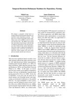
Figure 2: The next child, Ra(r3), is generated with

probability 7~(R3(r3)
[ P,H, h, distancer(2)).
The
distance
is a function of the surface string from the
word after h to the last word of R2, inclusive. In
principle the model could condition on any struc-
ture dominated by H, R1 or R2.
2.2 Model 2: The complement/adjunct
distinction and subcategorisation
The tree in figure 1 is an example of the importance
of the complement/adjunct distinction. It would be
useful to identify "Marks" as a subject, and "Last
week" as an adjunct (temporal modifier), but this
distinction is not made in the tree, as both NPs are
in the same position 5 (sisters to a VP under an S
node). From here on we will identify complements
by attaching a "-C" suffix to non-terminals fig-
ure 3 gives an example tree.
TOP
1
S(bought)
NP(w~ought)
Last week Marks
VBD NP-C(Brooks)
I l
bought Brooks
Figure 3: A tree with the "-C" suffix used to identify
complements. "Marks" and "Brooks" are in subject
and object position respectively. "Last week" is an

adjunct.
A post-processing stage could add this detail to
the parser output, but we give two reasons for mak-
ing the distinction while parsing: First, identifying
complements is complex enough to warrant a prob-
abilistic treatment. Lexical information is needed
5Except "Marks" is closer to the VP, but note that
"Marks" is also the subject in "Marks last week bought
Brooks".
for example, knowledge that "week '' is likely to
be a temporal modifier. Knowledge about subcat-
egorisation preferences for example that a verb
takes exactly one subject is also required. These
problems are not restricted to NPs, compare "The
spokeswoman said (SBAR that the asbestos was
dangerous)" vs. "Bonds beat short-term invest-
ments (SBAR because the market is down)", where
an SBAR headed by "that" is a complement, but an
SBAI:t headed by "because" is an adjunct.
The second reason for making the comple-
ment/adjunct distinction while parsing is that it
may help parsing accuracy. The assumption that
complements are generated independently of each
other often leads to incorrect parses see figure 4
for further explanation.
2.2.1 Identifying Complements and
Adjuncts in the Penn Treebank
We add the "-C" suffix to all non-terminals in
training data which satisfy the following conditions:
1. The non-terminal must be: (1) an NP, SBAR,

or S whose parent is an S; (2) an NP, SBAR, S,
or VP whose parent is a VP; or (3) an S whose
parent is an SBAR.
2. The non-terminal must
not
have one of the fol-
lowing semantic tags: ADV, VOC, BNF, DIR,
EXT, LOC, MNR, TMP, CLR or PRP. See
(Marcus et al. 94) for an explanation of what
these tags signify. For example, the NP "Last
week" in figure 1 would have the TMP (tempo-
ral) tag; and the SBAR in "(SBAR because the
market is down)", would have the ADV (adver-
bial) tag.
In addition, the first child following the head of a
prepositional phrase is marked as a complement.
2.2.2 Probabilities over Subcategorisation
Frames
The model could be retrained on training data
with the enhanced set of non-terminals, and it
might learn the lexical properties which distinguish
complements and adjuncts ("Marks" vs "week", or
"that" vs. "because"). However, it would still suffer
from the bad independence assumptions illustrated
in figure 4. To solve these kinds of problems, the gen-
erative process is extended to include a probabilistic
choice of left and right subcategorisation frames:
1. Choose a head H with probability
~H(H[P, h).
2. Choose left and right subcat frames,

LC
and
RC,
with probabilities
7)~c(LC [ P, H, h)
and
18
I. (a) Incorrect S
(b)
Correct S
NP-C VP
NP-C NP-C
VP
I I ~ f ~.
was ADJP
NP NP
Dreyfus the best fund was ADJP [
I I I low
low Dreyfus the best fund
2. (a) Incorrect S (b) Correct S
NP-C VP
NP-C VP l
I ~ The
issue
/ ~
The
issue was
NP-C
w -C NP VP
a bill a bill

funding NP-C funding NP-C
I I
Congress
Congress
Figure 4: Two examples where the assumption that modifiers are generated independently of each
other leads to errors. In (1) the probability of generating both "Dreyfus" and "fund" as sub-
jects, 7~(NP-C(Dreyfus) I S,VP,was) * T'(NP-C(fund) I S,VP,was) is unreasonably high. (2) is similar:
7 ~ (NP-C (bill), VP-C (funding) I VP, VB, was) = P(NP-C (bill) I VP, VB, was) * 7~(VP-C (funding) I VP, VB, was)
is a bad independence assumption.
Prc(RCIP, H,h ). Each subcat frame is a
multiset 6 specifying the complements which the
head requires in its left or right modifiers.
3. Generate the left and right modifiers with prob-
abilities 7)l(Li, li I H, P, h, distancet(i - 1), LC)
and 7~r (R~, ri I H, P, h, distancer(i - 1), RC) re-
spectively. Thus the subcat requirements are
added to the conditioning context. As comple-
ments are generated they are removed from the
appropriate subcat multiset. Most importantly,
the probability of generating the STOP symbol
will be 0 when the subcat frame is non-empty,
and the probability of generating a complement
will be 0 when it is not in the subcat frame;
thus all and only the required complements will
be generated.
The probability of the phrase S(bought)->
NP(week) NP-C(Marks) VP(bought)is now:
7)h(VPIS,bought) x
to({NP-C} I S,VP,bought) x t S,VP,bought) ×
7~/(NP-C(Marks) IS ,VP,bought, {NP-C}) x

7:~I(NP(week) I S ,VP ,bought, {}) x
7)l(STOe I S ,ve ,bought, {}) ×
Pr(STOP I S, VP,bought, {})
Here the head initially decides to take a sin-
gle NP-C (subject) to its left, and no complements
~A rnultiset, or bag, is a set which may contain du-
plicate non-terminal labels.
to its right.
NP-C(Marks)
is immediately gener-
ated as the required subject, and NP-C is removed
from LC, leaving it empty when the next modi-
fier, NP(week) is generated. The incorrect struc-
tures in figure 4 should now have low probabil-
ity because
~Ic({NP-C,NP-C}
[ S,VP,bought) and
"Prc({NP-C,VP-C} I VP,VB,was) are small.
2.3 Model 3: Traces and Wh-Movement
Another obstacle to extracting predicate-argument
structure from parse trees is wh-movement. This
section describes a probabilistic treatment of extrac-
tion from relative clauses. Noun phrases are most of-
ten extracted from subject position, object position,
or from within PPs:
Example 1 The store (SBAR which TRACE
bought Brooks Brothers)
Example 2 The store (SBAR which Marks bought
TRACE)
Example 3 The store (SBAR which Marks bought

Brooks Brothers/tom TRACE)
It might be possible to write rule-based patterns
which identify traces in a parse tree. However, we
argue again that this task is best integrated into
the parser: the task is complex enough to warrant
a probabilistic treatment, and integration may help
parsing accuracy. A couple of complexities are that
modification by an SBAR does not always involve
extraction (e.g., "the fact (SBAR that besoboru is
19
NP(store)
NP(store) SBAR(that)(+gap)
The store
WHNP(that)
WDT
I
that
(i) NP -> NP
(2) SBAR(+gap)
-> WHNP
(3) S(+gap) -> NP-C
(4) VP(+gap) -> VB
S(bought )(-}-gap)
N P-C(~ht) ( {-gap)
I B~w
Marks
V eek)
I I
bought last week
SBAR(+gap)

S-C(+gap)
VP(+gap)
TRACE NP
Figure 5: A
+gap
feature can be added to non-terminals to describe NP extraction. The top-level NP
initially generates an SBAR modifier, but specifies that it must contain an NP trace by adding the
+gap
feature. The gap is then passed down through the tree, until it is discharged as a
TRACE
complement to
the right of
bought.
played with a ball and a bat)"), and it is not un-
common for extraction to occur through several con-
stituents, (e.g., "The changes (SBAR that he said
the government was prepared to make TRACE)").
The second reason for an integrated treatment
of traces is to improve the parameterisation of the
model. In particular, the subcategorisation proba-
bilities are smeared by extraction. In examples 1, 2
and 3 above 'bought' is a transitive verb, but with-
out knowledge of traces example 2 in training data
will contribute to the probability of 'bought' being
an intransitive verb.
Formalisms similar to GPSG (Gazdar et al. 95)
handle NP extraction by adding a
gap
feature to
each non-terminal in the tree, and propagating gaps

through the tree until they are finally discharged as a
trace complement (see figure 5). In extraction cases
the Penn treebank annotation co-indexes a TRACE
with the WHNP head of the SBAR, so it is straight-
forward to add this information to trees in training
data.
Given that the LHS of the rule has a gap, there
are 3 ways that the gap can be passed down to the
RHS:
Head The gap is passed to the head of the phrase,
as in rule (3) in figure 5.
Left, Right The gap is passed on recursively to one
of the left or right modifiers of the head, or is
discharged as a
trace
argument to the left/right
of the head. In rule (2) it is passed on to a right
modifier, the S complement. In rule (4) a
trace
is generated to the right of the head VB.
We specify a parameter
7~c(GIP, h, H)
where G
is either Head, Left or Right. The generative pro-
cess is extended to choose between these cases after
generating the head of the phrase. The rest of the
phrase is then generated in different ways depend-
ing on how the gap is propagated: In the Head
case the left and right modifiers are generated as
normal. In the Left, Right cases a

gap
require-
ment is added to either the left or right SUBCAT
variable. This requirement is fulfilled (and removed
from the subcat list) when a trace or a modifier
non-terminal which has the
+gap
feature is gener-
ated. For example, Rule (2), SBAR(that) (+gap) ->
WHNP(that) S-C(bought) (+gap), has probability
~h (WHNP I SBAR, that) × 7~G (Right I SBAR, WHNP, that) x
T~LC({} I SBAR,WHNP,that) x
T'Rc({S-C}
[ SBAR,WHNP, that) x
7~R (S-C (bought) (+gap) [ SBAR, WHNP, that, {S-C, +gap}) x
7~R(STOP I SBAR,WHNP,that, {}) x
PC (STOP I SBAR, WHNP, that, { })
Rule (4), VP(bought) (+gap) -> VB(bought)
TRACE NP (week), has probability
7~h(VB I VP,bought) x PG(Right I VP,bought,VB) x
PLC({} I VP,bought,VB) x ~PRc({NP-C} I vP,bought,VB) x
7~R(TRACE I VP,bought,VB, {NP-C, +gap}) x
PR(NP(week) I VP,bought ,VB, {}) ×
7)L(STOP I VP,bought,VB, {}) x
7~R (STOP I VP ,bought ,VB, {})
In rule (2) Right is chosen, so the
+gap
requirement
is added to
RC.

Generation of S-C(bought)(+gap)
20
(a) H(+) =~ P(-)
• H(+)
Prob =X Pr£b =
X'X~H(HIP, )
(b) P(-) + Ri(+) =~
H R1
Prob -= X Prob = Y
Figure 6: The life of a constituent in the chart.
(c) P(-) =~ P(+)
Prob = X
Prob = X
X'PL(STOP I )
xPR(STOP I )
P(-)
• . H R1 Ri
Prob = X x Y x
~R(Ri(ri) I P,H, )
(+) means a constituent is complete (i.e. it includes the
stop probabilities), (-) means a constituent is incomplete. (a) a new constituent is started by projecting a
complete rule upwards; (b) the constituent then takes left and right modifiers (or none if it is unary). (c)
finally,
STOP
probabilities are added to complete the constituent.
Back-off
"PH(H
I"-) Pa(G I )
PL~(Li(It,)
I )

Level
PLc(LC t )
Pm(Ri(rti) I )
7)Rc(RC I )
1 P, w, t P, H, w, t P, H, w, t, A, LC
2 P, t P, H, t P, H, t, A, LC
3 P P, H P, H, &, LC
4
PL2(lwi l )
PR2(rwi I )
Li, Iti,
P, H, w, t, A, LC
L,, lti,
P, H, t, A, LC
LI, lti
It~
Table 1: The conditioning variables for each level of back-off. For example, T'H estimation interpolates
el = ~°H(H I P, w, t), e2 = 7~H(H I P, t),
and
e3 = PH(H I P). A
is the distance measure.
:ulfills both the S-C and
+gap
requirements in
RC.
In rule (4) Right is chosen again. Note that gen-
eration of
trace
satisfies both the NP-C and
+gap

subcat requirements.
3 Practical Issues
3.1 Smoothing and Unknown Words
Table 1 shows the various levels of back-off for each
type of parameter in the model. Note that we de-
compose
"PL(Li(lwi,lti) I P, H,w,t,~,LC)
(where
lwi
and
Iti
are the word and POS tag generated
with non-terminal Li, A is the distance measure)
into the product
79L1(Li(lti) I P, H,w,t, Zx,LC)
x
7~ L2(lwi ILi, lti, 19, H, w, t, A, LC),
and then smooth
these two probabilities separately (Jason Eisner,
p.c.). In each case 7 the final estimate is
e Ale1 +
(1 - &l)(A2e2 + (1 - &2)ea)
where ex, e2 and e3 are maximum likelihood esti-
mates with the context at levels 1, 2 and 3 in the
table, and ,kl, ,k2 and )~3 are smoothing parameters
where 0 _< ,ki _< 1. All words occurring less than 5
times in training data, and words in test data which
rExcept cases L2 and R2, which have 4 levels, so that
e = ~let + (1 *X1)()~2e2 + (1 - ,~2)(&3e3 + (1
- ~3)e4)).

have never been seen in training, are replaced with
the "UNKNOWN" token. This allows the model to
robustly handle the statistics for rare or new words.
3.2 Part of Speech Tagging and Parsing
Part of speech tags are generated along with the
words in this model. When parsing, the POS tags al-
lowed for each word are limited to those which have
been seen in training data for that word. For un-
known words, the output from the tagger described
in (Ratnaparkhi 96) is used as the single possible tag
for that word. A CKY style dynamic programming
chart parser is used to find the maximum probability
tree for each sentence (see figure 6).
4 Results
The parser was trained on sections 02 - 21 of the Wall
Street Journal portion of the Penn Treebank (Mar-
cus et al. 93) (approximately 40,000 sentences), and
tested on section 23 (2,416 sentences). We use the
PAR.SEVAL measures (Black et al. 91) to compare
performance:
Labeled Precision =
number of correct constituents in proposed parse
number of constituents in proposed parse
21
MODEL
(Magerman 95)
(Collins 96)
Model 1
Model 2
Model 3

~ce~) 2 CBs
84.6% 84.9% 1.26 56.6% 81.4% 84.0% 84.3% 1.46 54.0%
85.8% 86.3% 1.14 59.9% 83.6% 85.3% 85.7% 1.32 57.2%
87.4% 88.1% 0.96 65.7% 86.3% 86.8% 87.6% 1.11 63.1%
88.1% 88.6% 0.91 66.5% 86.9% 87.5% 88.1% 1.07 63.9%
88.1% 88.6% 0.91 66.4% 86.9% 87.5% 88.1% 1.07 63.9%
78.8%
80.8%
84.1%
84.6%
84.6%
Table 2: Results on Section 23 of the WSJ Treebank. LR/LP = labeled recall/precision. CBs is the average
number of crossing brackets per sentence. 0 CBs, < 2 CBs are the percentage of sentences with 0 or < 2
crossing brackets respectively.
Labeled Recall
-~
number o/ correct constituents in proposed parse
number of constituents in treebank parse
Crossing Brackets number of con-
stituents which violate constituent boundaries
with a constituent in the treebank parse.
For a constituent to be 'correct' it must span the
same set of words (ignoring punctuation, i.e. all to-
kens tagged as commas, colons or quotes) and have
the same label s as a constituent in the treebank
parse. Table 2 shows the results for Models 1, 2 and
3. The precision/recall of the traces found by Model
3 was 93.3%/90.1% (out of 436 cases in section 23
of the treebank), where three criteria must be met
for a trace to be "correct": (1) it must be an argu-

ment to the correct head-word; (2) it must be in the
correct position in relation to that head word (pre-
ceding or following); (3) it must be dominated by the
correct non-terminal label. For example, in figure 5
the trace is an argument to bought, which it fol-
lows, and it is dominated by a VP. Of the 436 cases,
342 were string-vacuous extraction from subject po-
sition, recovered with 97.1%/98.2% precision/recall;
and 94 were longer distance cases, recovered with
76%/60.6% precision/recall 9
4.1 Comparison to previous work
Model 1 is similar in structure to (Collins 96)
the major differences being that the "score" for each
bigram dependency is 7't(L{,liIH, P,
h, distancet)
8(Magerman 95) collapses ADVP and PRT to the same
label, for comparison we also removed this distinction
when calculating scores.
9We exclude infinitival relative clauses from these fig-
ures, for example "I called a plumber TRACE to fix the
sink" where 'plumber' is co-indexed with the trace sub-
ject of the infinitival. The algorithm scored 41%/18%
precision/recall on the 60 cases in section 23 but in-
finitival relatives are extremely difficult even for human
annotators to distinguish from purpose clauses (in this
case, the infinitival could be a purpose clause modifying
'called') (Ann Taylor, p.c.)
rather than Pz(Li,
P, H I li, h, distancel),
and that

there are the additional probabilities of generat-
ing the head and the
STOP
symbols for each con-
stituent. However, Model 1 has some advantages
which may account for the improved performance.
The model in (Collins 96) is deficient, that is for
most sentences S, Y~T 7~( T ] S) < 1, because prob-
ability mass is lost to dependency structures which
violate the hard constraint that no links may cross.
For reasons we do not have space to describe here,
Model 1 has advantages in its treatment of unary
rules and the distance measure. The generative
model can condition on any structure that has been
previously generated we exploit this in models 2
and 3 whereas (Collins 96) is restricted to condi-
tioning on features of the surface string alone.
(Charniak 95) also uses a lexicalised genera-
tive model. In our notation, he decomposes
P(RHSi l LHSi) as "P(R,~ R1HL1 Lm ] P,h) x
1-L=I ~ 7~(r~l P, Ri, h) x I-L=l m 7)(lil P, Li, h).
The
Penn treebank annotation style leads to a very
large number of context-free rules, so that directly
estimating
7~(R R1HL1 Lm I P, h)
may lead to
sparse data problems, or problems with coverage
(a rule which has never been seen in training may
be required for a test data sentence). The com-

plement/adjunct distinction and traces increase the
number of rules, compounding this problem.
(Eisner 96) proposes 3 dependency models, and
gives results that show that a generative model sim-
ilar to Model 1 performs best of the three. However,
a pure dependency model omits non-terminal infor-
mation, which is important. For example, "hope" is
likely to generate a VP(T0) modifier (e.g., I hope
[VP to sleep]) whereas "'require" is likely to gen-
erate an S(T0) modifier (e.g., I require IS Jim to
sleep]), but omitting non-terminals conflates these
two cases, giving high probability to incorrect struc-
tures such as "I hope [Jim to sleep]" or "I require [to
sleep]". (Alshawi 96) extends a generative depen-
dency model to include an additional state variable
which is equivalent to having non-terminals his
22
suggestions may be close to our models 1 and 2, but
he does not fully specify the details of his model, and
doesn't give results for parsing accuracy. (Miller et
al. 96) describe a model where the RHS of a rule is
generated by a Markov process, although the pro-
cess is not head-centered. They increase the set of
non-terminals by adding semantic labels rather than
by adding lexical head-words.
(Magerman 95; Jelinek et al. 94) describe a
history-based approach which uses decision trees to
estimate
7a(T[S).
Our models use much less sophis-

ticated n-gram estimation methods, and might well
benefit from methods such as decision-tree estima-
tion which could condition on richer history than
just surface distance.
There has recently been interest in using
dependency-based parsing models in speech recog-
nition, for example (Stolcke 96). It is interesting to
note that Models 1, 2 or 3 could be used as lan-
guage models. The probability for any sentence can
be estimated as
P(S) = ~~.TP(T,S),
or (making
a Viterbi approximation for efficiency reasons) as
7)(S) .~ P(Tb~st, S).
We intend to perform experi-
ments to compare the perplexity of the various mod-
els, and a structurally similar 'pure' PCFG 1°.
5
Conclusions
This paper has proposed a generative, lexicalised,
probabilistic parsing model. We have shown that lin-
guistically fundamental ideas, namely subcategori-
sation and wh-movement, can be given a statistical
interpretation. This improves parsing performance,
and, more importantly, adds useful information to
the parser's output.
6 Acknowledgements
I would like to thank Mitch Marcus, Jason Eisner,
Dan Melamed and Adwait Ratnaparkhi for many
useful discussions, and comments on earlier versions

of this paper. This work has also benefited greatly
from suggestions and advice from Scott Miller.
References
H. Alshawi. 1996. Head Automata and Bilingual
Tiling: Translation with Minimal Representa-
tions.
Proceedings of the 3~th Annual Meeting
of the Association for Computational Linguistics,
pages 167-176.
E. Black et al. 1991. A Procedure for Quantita-
tively Comparing the Syntactic Coverage of En-
glish Grammars.
Proceedings of the February 1991
DARPA Speech and Natural Language Workshop.
1°Thanks to one of the anonymous reviewers for sug-
gesting these experiments.
T. L. Booth and R. A. Thompson. 1973.
Applying
Probability Measures to Abstract Languages.
IEEE
Transactions on Computers, C-22(5), pages 442-
450.
E. Charniak. 1995.
Parsing with Context-Free Gram-
mars and Word Statistics.
Technical Report CS-
95-28, Dept. of Computer Science, Brown Univer-
sity.
N. Chomsky. 1957.
Syntactic Structures,

Mouton,
The Hague.
M. J. Collins. 1996. A New Statistical Parser Based
on Bigram Lexical Dependencies.
Proceedings o/
the 34th Annual Meeting o/ the Association for
Computational Linguistics,
pages 184-191.
J. Eisner. 1996. Three New Probabilistic Models for
Dependency Parsing: An Exploration.
Proceed-
ings o/ COLING-96,
pages 340-345.
G. Gazdar, E.H. Klein, G.K. Pullum, I.A. Sag. 1985.
Generalized Phrase Structure Grammar.
Harvard
University Press.
F. Jelinek, J. Lafferty, D. Magerman, R. Mercer, A.
Ratnaparkhi, S. Roukos. 1994. Decision Tree Pars-
ing using a Hidden Derivation Model.
Proceedings
o/ the 1994 Human Language Technology Work-
shop,
pages 272-277.
D. Magermaa. 1995. Statistical Decision-Tree Mod-
els for Parsing.
Proceedings o/ the 33rd Annual
Meeting o] the Association for Computational
Linguistics,
pages 276-283.

M. Marcus, B. Santorini and M. Marcinkiewicz.
1993. Building a Large Annotated Corpus of En-
glish: the Penn Treebank.
Computational Linguis-
tics,
19(2):313-330.
M. Marcus, G. Kim, M. A. Marcinkiewicz, R.
MacIntyre, A. Bies, M. Ferguson, K. Katz, B.
Schasberger. 1994. The Penn Treebank: Annotat-
ing Predicate Argument Structure.
Proceedings of
the 1994 Human Language Technology Workshop,
pages 110~115.
S. Miller, D. Staliard and R. Schwartz. 1996. A
Fully Statistical Approach to Natural Language
Interfaces.
Proceedings o/ the 34th Annual Meeting
of the Association for Computational Linguistics,
pages 55-61.
A. Ratnaparkhi. 1996. A Maximum Entropy Model
for Part-Of-Speech Tagging.
Conference on Em-
pirical Methods in Natural Language Processing.
A. Stolcke. 1996. Linguistic Dependency Modeling.
Proceedings of ICSLP 96, Fourth International
Conference on Spoken Language Processing.
23